Technical Report: A New Hopping Controller for Highly Dynamical Bipeds* Thanks: *This work was supported in part by the US Army Research Office under grant W911NF-17-1-0229.Thanks: ¹Mechanical Engineering and Applied Mechanics, University of Pennsylvania, PA, USA. srozen01@seas.upenn.eduThanks: ²Electrical and Systems Engineering, University of Pennsylvania, PA,USA. kod@seas.upenn.edu

Shane Rozen-Levy Daniel E. Koditschek

Abstract

We present angle of attack control, a novel control strategy for a hip energized Penn Jerboa. The energetic losses from damping are counteracted by aligning most of the velocity at touchdown in the radial direction and the fore-aft velocity is controlled by using the hip torque to control to a target angular momentum. The control strategy results in highly asymmetric leg angle trajectories, thus avoiding the traction issues that plague hip actuated SLIP. Using a series of assumptions we find an analytical expression for the fixed points of an approximation to the hopping return map relating the design parameters to steady state gait performance. The hardware robot demonstrates stable locomotion with speeds ranging from 0.4 m/s to 2.5 m/s (2 leg lengths/s to 12.5 leg lengths/s) and heights ranging from 0.21 m to 0.27 m (1.05 leg lengths to 1.35 leg lengths). The performance of the empirical trials is well approximated by the analytical predictions.

I Introduction

In contrast to many popular contemporary legged robots [1, 2, 3], the Penn Jerboa (fig. 1(a)) is a dramatically underactuated biped: it has 12 DoF (degrees of freedom) and only 4 direct drive actuators [4, 5, 6]. Moreover, unlike many bipeds, it features small point toes rather than flat feet [7]. Jerboa’s consequent high power density (43.2 w/kg [6]) and its unusual recourse to a high powered (two DoF) tail at the expense of affording only one actuator at each hip of its passive spring loaded legs provokes the question of whether and how its largely dynamical and comparatively more energetic regime of operation can offer performance competitive with that of more conventional legged designs.

Refer to caption — (a) The Penn Jerboa [8], a tailed biped with springy legs and only four actuators: one driving the leg angle at each hip; and two controlling the 2 DoF tail.

Because its extreme underactuation precludes recourse to popular control approaches that assume the availability of arbitrary ground reaction forces subject to linear frictional constraints [9, 10, 11, 12, 13], prior work on Jerboa has built on the long tradition of anchoring compositions of dynamical templates [14, 15, 16, 17]. This paper introduces a new entry to the catalogue of spring loaded inverted pendulum (SLIP) [18] template controllers, offering a novel, model-relaxed strategy for controlling the speed and height of Jerboa using its hip motors. This leaves the tail free to control the pitch and roll (future work). Compared to previous work on Jerboa, this control strategy allows the robot to hop faster with just as much height — albeit potentially with the need for greater traction since the original tail-energized hopping mode [8] explicitly drives energy down the leg shaft, increasing the normal component of the ground reaction forces.

We find fixed points and prove stability for an approximate model of closed loop hopping generated by this control strategy by using assumptions to construct an analytical return map. The fixed points of this simplified system effectively approximate the numerical fixed points of the unsimplified system allowing for an intuitive understanding of how the parameters affect the steady state operating regime of the robot. We test this control strategy in hardware showing a wide range of steady state operating regimes.

I-A Background Literature

Since Raibert, the SLIP model has been used to study legged locomotion[19, 20, 21, 22, 23]. Raibert controlled SLIP-like robots with a fixed thrust in stance to energize hopping and used the touchdown angle to control speed.

Due to the simple nature of the flight map and resets, much of the analytical work on SLIP has focused on approximating the stance map [24, 25]. The fixed points of the analytical return map serve as a map from the many dimensional parameter space to the operating conditions of the robot [26].

Inspired by the work in [24], Ankarali et al. develops an analytical approximation of the stance map for SLIP with damping and gravity by linearizing gravity, yielding a conservation of angular momentum [25]. Ankarali et al. then approximates the effect of gravity by iteratively estimating the average angular momentum [27].

They extend the results to the stance map for hip energized SLIP by taking the open loop hip torque into account when calculating the average angular momentum[28, 29]. They use inverse dynamics to find the hip torque to get to the target energy and solve an optimization problem for the touchdown angle. Ankarali et al. are unable to analytically find fixed points of the return map and they never implemented the control strategy on a physical robot.

In addition to the work in [28, 29], there have been a handful of papers exploring hip energized hopping for SLIP-like robots[30, 31, 32].

I-B Contributions and Organization

With the goal of developing a simple, analytically tractable, control strategy for a hip energized SLIP-like robot, this paper makes three contributions: (i) a simple and novel control strategy for hip energized SLIP where energetic losses from damping are counteracted by choosing a touchdown angle that puts most of the speed at touchdown in the radial direction (eq. 3) and the leg angle is energized using the hip torque (eq. 4); (ii) a closed form analytical approximation of the fixed points for a simplified model of SLIP under the new control strategy (eq. 8); (iii) an extensive empirical study of the implementation of the novel control strategy on the physical Jerboa robot [8].

This control strategy (i) allows for intuitive control of the fore-aft velocity(figure 3) and some control over the apex height (figure 3). The analytical predictions (ii) match the fixed points of the numerical return map(table III) and predict with reasonable accuracy the height and speed of the robot (fig 5, fig 5, table IV). The robot (iii) demonstrated stable locomotion with speeds ranging from 0.4 m/s to 2.5 m/s (2 leg lengths/s to 12.5 leg lengths/s) and heights ranging from 0.21 m to 0.27 m (fig 5, fig 5, fig 6).

Section II develops the approximations that yield a closed form return map. Section III introduces further simplifying assumptions affording simple closed form approximation of the fixed points of the return map and compares the accuracy of both relative to their counterparts arising from numerical integration of the original physical model (sec. III-B). Section IV demonstrates the performance of the controller on Jerboa. Section V wraps up the paper with a discussion of the key ideas and some future steps.

Symbol	Brief Description	Ref
$\theta$	leg angle	fig. 1(b)
$r$	leg length	fig. 1(b)
$m$	mass	fig. 1(b)
$k$	spring constant	fig. 1(b)
$\tau$	hip torque	fig. 1(b)
$b$	damping coefficient	fig. 1(b)
$r_{0}$	spring rest length	fig. 1(b)
$x$	fore-aft position	fig. 1(b)
$y$	height relative to ground	fig. 1(b)
$z^{s}$	the state in stance = $[r,\dot{r},\theta,\dot{\theta}]$	sec. II-A
$g$	acceleration due to gravity	eq. 1
$k_{\theta}$	angle of attack gain	eq. 3
$\theta_{\text{AoA}}$	angle of attack	eq. 3
$\bar{p}_{\theta}$	target angular momentum in stance	eq. 4
$z^{a}$	the state at apex = $[\dot{x},y]$	eq. 5

TABLE I: Symbol definitions

II Return Map

The ballistic modes (ascent and descent) of the SLIP model are completely integrable; hence the effort in constructing the return map whose fixed points are of interest lies in approximating its non-integrable stance mode map [33].

II-A Stance Map, Ascent Map, Descent Map, Resets

The non-integrability [34] of SLIP dynamics

\displaystyle\begin{bmatrix}\ddot{r}\\ \ddot{\theta}\end{bmatrix}=\begin{bmatrix}-k/m(r-r_{0})-b/m\dot{r}-g\cos(\theta)\\ \frac{-2\dot{r}\dot{\theta}}{r}+g/r\sin(\theta)+\frac{\tau}{mr^{2}}\end{bmatrix}

(1)

introduces the burden of imposing simplifying assumptions yielding physically effective approximations for designers seeking closed form expression and stability guarantees for steady state gaits.

In order to get integrable dynamics we start with two assumptions inspired by the work in [27].

Assumption 1

Since we control to a target angular momentum, $\bar{p_{\theta}}$ , the angular momentum is constant and equal to the target angular momentum.

Assumption 2

The leg angle is small, thus gravity acts radially.

As in [27], we take a Taylor series approximation of the $1/r^{3}$ and $1/r^{2}$ terms in the post assumption dynamics (eq. 9) centered at $r=r_{g}$ , where $r_{g}=r0-mg/k$ , yielding

\displaystyle\begin{bmatrix}\ddot{r}\\ \dot{\theta}\end{bmatrix}=\begin{bmatrix}\frac{\bar{p_{\theta}}^{2}}{m^{2}r_{g}^{3}}-(\frac{3\bar{p_{\theta}}^{2}}{m^{2}r_{g}^{4}}+\frac{k}{m})(r-r_{g})-\frac{b}{m}\dot{r}\\ \frac{3\bar{p_{\theta}}}{mr_{g}^{2}}-\frac{2\bar{p_{\theta}}}{mr_{g}^{3}}r\end{bmatrix},

(2)

a 1 DoF linear time invariant damped harmonic oscillator in $r$ feeding forward to excite a first order linear time invariant leg angle integrator in $\theta$ . For the closed form solutions see (eq. 12, eq. 13, eq. 16).

Integrating (2) and following [28] to obtain $t_{lo}$ , the liftoff time, yields the stance map approximation, $\Psi_{s}\mathbb{:}\mathbb{R}^{3}\times S^{1}\rightarrow\mathbb{R}^{3}\times S^{1}$ , $\mathbb{:}z^{s}_{td}\mapsto z^{s}_{lo}$ , which we display in closed form below in eq. 6 after introducing a number of further simplifying assumptions.

II-A1 Ascent, Descent, and Reset Maps

Due to the single point mass, SLIP follows a ballistic trajectory in flight. Apex is defined by $\dot{y}=0$ , and touchdown occurs when the toe contacts the ground.

Similarly due to the massless foot and springy legs, the reset maps do not have to handle impacts. Thus, the resets convert between the polar coordinates used in stance and the cartesian coordinates used in flight. See (app. A-E, app. A-F) for details on the resets, ascent, and descent maps.

II-B Angular and Radial Control Policies

Early on in our experiments, we found that Raibert stepping [23] did not work well for hip energized hopping because the Coriolis term did not provide sufficient coupling for the hip torque to counteract the radial damping.

Angle of attack control (hereafter, AoA) counteracts the energetic losses from damping by choosing a touchdown angle that puts most of kinetic energy at touchdown into the $\dot{r}$ component; as a result $|\dot{\theta}_{td}|$ is small. The hip torque then re-energizes $\theta$ directly, without relying on coupling.

Let $\theta_{td}=k_{\theta}\theta_{\text{AoA}}$ be the touchdown angle under AoA where $k_{\theta}$ is the gain on the touchdown angle (nominally 1) and $\theta_{\text{AoA}}$ is the angle of attack. $\theta_{\text{AoA}}:=\arctan{\frac{\dot{x}_{td}}{\dot{y}_{td}}}$ . Since $\dot{y}_{td}$ varies with $\theta_{td}$ , this yields the constraint equation

\theta_{\text{AoA}}=\Phi(\theta_{\text{AoA}}):=\arctan\frac{\dot{x}}{\sqrt{2E_{v}/m-2gr_{0}\cos(k_{\theta}\theta_{\text{AoA}})}},

(3)

where $E_{v}:=1/2m\dot{y}^{2}+mgy$ is the vertical energy. An approximation to the implicit function for $\theta_{AoA}$ satisfying constraint 3 is presented in (eq. 22).

The AoA gain, $k_{\theta}$ , is nominally between $0$ and $1$ . $k_{\theta}<1$ corresponds to having some initial angular velocity at touchdown. A $k_{\theta}>1$ corresponds to having angular velocity in the opposite direction of travel at touchdown. For this paper we will restrict $k_{\theta}\in[0,1]$ .

The angular control policy is a PID + feed forward loop which control the leg to a target angular momentum.

\tau_{j}=k_{p}(\bar{p}_{\theta}-p_{\theta,j})+k_{i}\sum_{i=0}^{j}(\bar{p}_{\theta}-p_{\theta,i})-k_{d}\dot{p}_{\theta,j}-mgr_{j}\sin{\theta_{j}}

(4)

II-C Constructing the Return Map

Given the stance map ( $\Psi_{s}$ , sec II-A), resets( ${{}^{s}R^{f}},{{}^{f}R^{s}}$ , sec. II-A1), ascent map( $\Psi_{a}$ , sec. II-A1), and descent map( $\Psi_{d}$ , sec. II-A1), we construct the apex coordinate return map by composing the analytical functions.

	$\displaystyle P:$	$\displaystyle\mathbb{R}^{2}\rightarrow\mathbb{R}^{2}:=\Psi_{a}\circ{{}^{f}R^{s}}\circ\Psi_{s}\circ{{}^{s}R^{f}}\circ\Psi_{d}$
	$\displaystyle\mathbb{:}$	$\displaystyle z^{a}_{k}\mapsto z^{a}_{k+1}$		(5)

III Fixed Points and Stability of the Analytical Return Map

Notwithstanding the closed form expression for $P$ represented by (5), developing an intuitively useful closed form expression for its fixed points is facilitated by the following simplifying assumptions.

Assumption 3

Across all fixed points, the nondimensionalized time of stance, $t_{lo}/\omega_{d}$ is constant.

Assumption 4

$r_{lo}\approx r_{0}$ . ¹¹ 1 Based on the radial velocity at liftoff, the spring constant, and the damping, this is accurate within 2mm.

Using these assumptions the stance map, $\Psi_{s}$ derived in Sec. II-A takes takes the form

\displaystyle z^{s}_{lo}=\begin{bmatrix}r_{0}\\ C_{1}\dot{r}_{td}+C_{2}\\ \theta_{td}+C_{3}\dot{r}_{td}+C_{4}\\ \bar{p}_{\theta}/(mr_{0}^{2})\end{bmatrix},

(6)

where $C_{1},...C_{4}$ are defined in (eq. 23-eq. 26).

Assumption 5

$\cos{\theta}\approx 1-\frac{\theta^{2}}{2}$ and $\sin{\theta}\approx\theta$ (see figure 6 for evidence that this assumption is valid ).

Assumption 6

The change in gravitational potential energy between touchdown and liftoff is negligible compared to the kinetic energy

Assumption 7

$\dot{\theta}_{td}\approx-\dot{r}_{td}/r_{0}\tan{(\theta_{\text{offset}})}$ where $\theta_{\text{offset}}:=\bar{p}_{\theta}/0.7\frac{\pi}{4}(1-k_{\theta})$ .

See (app. B-B) for a derivation of this assumption. Total energy and fore-aft velocity are conserved in flight, thus at the fixed point we impose the constraints, $E_{td}=E_{lo}$ and $\dot{x}_{td}=\dot{x}_{lo}$ yielding quadratic polynomials in the touchdown state variables (eq. 27, eq. 28). The constraint on energy yields a quadratic polynomial in $\dot{r}^{*}_{td}$ whose coefficients, $a_{r},b_{r},c_{r}$ are given by elementary functions of the physical parameters and control inputs listed in (eq. 29). In turn, the constraint on fore-aft velocity yields a quadratic polynomial in $\theta^{*}_{td}$ whose coefficients, $a_{\theta},b_{\theta},c_{\theta}$ are given by similar functions that now also depend upon the value of $\dot{r}^{*}_{td}$ (eq. 30-eq. 32). Thus, the fixed points of $P$ (eq. 5) are given as

\displaystyle\begin{bmatrix}\dot{r}^{*}_{td}\\ \theta^{*}_{td}\\ \dot{\theta}^{*}_{td}\end{bmatrix}=F(\bar{p}_{\theta},k_{\theta}):=\begin{bmatrix}R(\bar{p}_{\theta},k_{\theta}))\\ \Theta(\bar{p}_{\theta},k_{\theta})\\ \Xi(\bar{p}_{\theta},k_{\theta})\end{bmatrix}

(7)

where

	$\displaystyle R(\bar{p}_{\theta},k_{\theta})$	$\displaystyle:=Q_{-}\big(a_{r}(\bar{p}_{\theta},k_{\theta}),b_{r},c_{r}(\bar{p}_{\theta})\big)$
	$\displaystyle\Theta(\bar{p}_{\theta},k_{\theta})$	$\displaystyle:=Q_{+}\big(a_{\theta}(R(\bar{p}_{\theta},k_{\theta}),\bar{p}_{\theta},k_{\theta}),$
		$\displaystyle b_{\theta}(R(\bar{p}_{\theta},k_{\theta}),\bar{p}_{\theta},k_{\theta}),c_{\theta}(R(\bar{p}_{\theta},k_{\theta}),\bar{p}_{\theta},k_{\theta})\big)$
	$\displaystyle\Xi(\bar{p}_{\theta},k_{\theta})$	$\displaystyle:=-R(\bar{p}_{\theta},k_{\theta})/r_{0}\tan(\theta_{\text{offset}})$

where $Q_{\pm}$ are the positive and negative roots of a quadratic polynomial (eq. 33).

Given the fixed point in touchdown coordinates, we map it backwards in time to get the apex coordinate fixed points:

{z^{a}}^{*}=\Psi_{d}^{-1}\circ({{}^{s}R^{f}})^{-1}([r_{0},F(\bar{p}_{\theta},k_{\theta})])

(8)

We check stability of the fixed points by evaluating the Jacobian of the return map and checking if its spectral radius is less than 1 at the fixed point.

III-A Plots of Analytical Fixed Points

Table II has the parameters used in the analytical return map. Figure 3 and 3 plot the apex fore-aft speed and height as a function of the control inputs, $\bar{p}_{\theta}$ and $k_{\theta}$ . The apex speed shows a significantly decoupling between $k_{\theta}$ and $\bar{p}_{\theta}$ ; $\bar{p}_{\theta}$ heavily effects the speed while $k_{\theta}$ has almost no effect on the speed. By using $\bar{p}_{\theta}=-m\dot{x}_{\text{des}}r_{0}$ (corresponding to speed when $\theta_{lo}=0$ ), the resulting relationship between the target and actual speed would be monotonic and zero at zero target speed.

$m$ (kg)	$3.3$
$r_{0}$ (m)	0.2
$k$ (N/m)	4000
$b$ (Ns/m)	20

TABLE II: Jerboa’s model parameters

Fig. 2: Apex velocity of fixed points predicted by the analytical return map (eq. 8) as functions of the control inputs

k_{\theta}

and

\bar{p}_{\theta}

. This plot shows a decoupling between

k_{\theta}

and

\bar{p}_{\theta}

; increasing

|\bar{p}_{\theta}|

increases the speed while changing

k_{\theta}

has almost no effect on the speed.

\bar{p}_{\theta}=-m\dot{x}_{\text{des}}r_{0}

is the line corresponding to the fore-aft velocity if

\theta_{lo}=0

. The accuracy of these fixed points relative to the numerically integrated values is presented in table III. The model parameters are in table II.

Fig. 3: Apex height of fixed points predicted by the analytical return map (eq. 8) as a function of the control inputs

k_{\theta}

and

\bar{p}_{\theta}

. Increasing

k_{\theta}

increases the apex height. Contrary to

k_{\theta}

\bar{p}_{\theta}

’s effect on the height is not monotonic. For a fixed

k_{\theta}

, there is a

\bar{p}_{\theta}

resulting in a maximum height. This corresponds to

\theta_{lo}=0

, thus a higher

|\bar{p}_{\theta}|

decreases

\dot{y}_{lo}

and a lower

|\bar{p}_{\theta}|

results in less energy to put into the radial subsystem. The accuracy of these fixed points relative to the numerically integrated values is presented in table III. The model parameters are in table II.

On the other hand, the apex height shows some coupling between $k_{\theta}$ and $\bar{p}_{\theta}$ . $k_{\theta}$ has a monotonic relationship with height, though increasing $|\bar{p}_{\theta}|$ increases $\partial y^{*}/\partial k_{\theta}$ . This should be thought of as for the higher $|\bar{p}_{\theta}|$ , $k_{\theta}$ has a larger affordance on height. The simple formulation of this control strategy, the decoupling in the control of fore-aft velocity, and the angle of attack gain’s consistent effect on height makes this control strategy ideal for hip energized SLIP.

III-B Accuracy of the Fixed Points

In order to validate our numerous assumption and evaluate the accuracy of the analytical return map, we compared its fixed points (eq. 8) to the fixed points of the numerical return map.

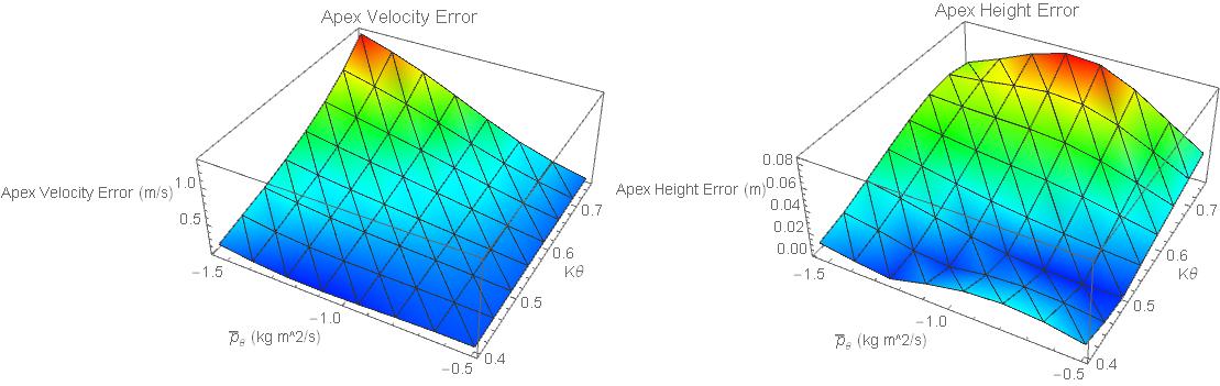
Table III is the error between the fixed points of the analytical return map and the fixed points of the numerical return map over a rectangular approximation of the robot’s operating regime, $\bar{p}_{\theta}\in[-0.5,-1.55]kgm^{2}/s$ , $k_{\theta}\in[0.4,0.75]$ . The error is mostly small over the operating regime except for the error in $\dot{x}$ when $|\bar{p}_{\theta}|$ and $k_{\theta}$ are large. These control inputs result in a large $\theta_{td}$ , thus violating assumptions 2, 5, and 6.

	RMS Error	Percent RMS Error
$\dot{x}$	0.488 m/s	20.3%
$y$	0.037 m	13.3%

TABLE III: Accuracy of the analytical return map’s predicted speed and height (eq. 8) compared to the numerical return map’s predicted speed and height over a rectangular approximation of the robot’s operating regime.

\bar{p}_{\theta}\in[-0.5,-1.55]kgm^{2}/s

k_{\theta}\in[0.3,0.75]

. The RMS error in the apex coordinates is small showing that the approximate analytical return map matches the numerical return map. The model parameters are in table II. See (fig 8) for plot of the error of the analytical return map’s fixed points compared to the numerical return map’s fixed points.

IV Experiments

In order to test angle of attack control, we implemented the controller on the boom-mounted, pitch-locked, Jerboa robot with its tail removed [8].

The control strategy works very well in hardware. The robot achieved speeds of up to 2.5 m/s (limited by kinematics) and heights of up to 0.27 m. The main failure modes were premature touchdown and failing to liftoff. The attached supplemental video has clips of Jerboa hopping at representative steady state set points across the operating regime. Fig. 5 and Fig. 5 contrast the analytical prediction of apex coordinate fixed point with empirical data taken at steady state.

IV-A Experimental Setup

The Jerboa robot weighs 3.3 kg, has a max hip torque of 7 Nm from 2 TMotor U8 [35], a 4000 N/m spring leg, and an operating voltage of 16.8 V from an offboard LiPo. Jerboa’s processor is a PWM mainboard from Ghost Robotics[36] which runs angle of attack control at 1 kHz.

IV-A1 Implementation Detail

Angle attack control requires an estimate of the robot’s velocity at liftoff (3). We estimated this value using a coarse derivative of the robot’s position estimated with the leg kinematics (touchdown to liftoff for fore-aft velocity, and bottom to liftoff for vertical velocity).

Additionally, the motors controllers on Jerboa did not have current/torque control, only voltage control. Fortunately we were still able to use a controller of the same form as eq. 4, though the constant on the gravity compensation term had to be manually tuned.

IV-B Empirical Fixed Points

We tested the robot with $\bar{p}_{\theta}\in[-0.4,-1.7]kgm^{2}/s$ and $k_{\theta}\in[0.3,0.75]$ . Figure 5 and 5 plot the apex coordinate fixed points for the control inputs that resulted in stable locomotion. Jerboa was able to hop at speeds ranging from 0.4 m/s (2 leg lengths/s) to 2.5 m/s (12.5 leg length/s). As was predicted by the analytical return map, the fore-aft speed is controlled by $\bar{p}_{\theta}$ . Additionally, the robot was able to hop at heights ranging from 0.21 m to 0.27 m. As with the analytical return map, the height is controlled by the $\bar{p}_{\theta}$ and $k_{\theta}$ where increasing $k_{\theta}$ increases the height. Table IV presents the error of the fixed points of the analytical return map compared to the empirical results.

	RMS Error	Percent	Max Error	Max Percent
		RMS Error		Error
$\dot{x}$	0.595 m/s	36.7%	1.328 m/s	82.0%
$y$	0.0264 m	11.6%	0.060 m	26.5%

TABLE IV: Accuracy of the analytical apex coordinate fixed points compared to the empirical fixed points over the robots operating regime. The analytical return map does an excellent job predicting

\dot{x}

and

y

in the low and middle operating range and deteriorates at the higher ranges of

k_{\theta}

and

\bar{p}_{\theta}

as shown in Figs. 5 & 5.

The analytical return map does an excellent job predicting the empirical fixed points. Not only are the trends preserved, but the actual values are fairly similar. The height is accurate to about 1/10 of a leg length and the error in speed is concentrated at the higher angular momentums.

IV-C Steady State Trajectories

Figure 6 shows the steady state trajectory of the robot with moderate speed and height. The angular momentum asymptotically converges to the target angular momentum over the course of stance without saturating the motors. The resulting leg angle trajectories are very asymmetric. $\theta_{td}\approx 0.45rad$ while $\theta_{lo}\approx 0rad$ . This means that the hip torque is always increasing the normal component of the ground reaction forces, rather than decreasing it. Even though $k_{\theta}<1$ , ${p_{\theta}}_{td}$ is opposite the direction of travel. This is likely caused by the impact at touchdown and the 4 bar linkage in the leg.

Fig. 6: A time domain trace of the robot hopping with

\bar{p}_{\theta}=-0.79kgm^{2}/s

and

k_{\theta}=0.64

. At touchdown the hip motors briefly saturate before dropping down to a lower voltage. Additionally, the leg angle trajectory is highly asymmetric (

\theta_{td}=0.45rad,\,\theta_{lo}=0.05rad

) which prevents slippage.

These plots also shows the validity of some of our earlier assumptions. For the lower $|\bar{p}_{\theta}|$ , the leg angle stays small. Although we assumed angular momentum is constant, it changes quickly over stance, always reaching or slightly overshooting $\bar{p}_{\theta}$ .

Figure 7 is the $r,\dot{r}$ limit cycle from the empirical trials for $\bar{p}_{\theta}=-1.1kgm^{2}/s$ and a step response of $k_{\theta}$ . This plot shows that the system to robust to changes in input and that increasing $k_{\theta}$ increases the energy in the radial subsystem.

Fig. 7: The

r,\dot{r}

limit cycle for

\bar{p}_{\theta}=-1.1kgm^{2}/s

and a step response of

k_{\theta}

. As predicted by the analytical results increasing

k_{\theta}

increases the energy in the radial subsystem.

V Conclusion

This paper presents a novel hip energized control strategy for a pitch constrained Jerboa. The control strategy allows Jerboa to hop at speeds of up 2.5 m/s. By constructing and validating an analytical return map we found a closed form expression for the fixed points giving insight into how the parameters affect the operating regime of the robot.

V-A Discussion

V-A1 Energizing the Radial Component Through Resets

With hip energized SLIP, the energetic losses enter through the radial dynamics while the energization happens in the leg angle dynamics. Since the only coupling in stance occurs through the Coriolis terms of the dynamics (which are typically very weak in regimes of physical interest), we energize the radial direction through a smart choice of reset map. By controlling around a touchdown angle that maximizes $|\dot{r}_{td}|$ (eq. 3), the radial direction can be energized at the cost of $\dot{\theta}_{td}$ . The leg angle is then re-energized using a hip torque. One side effect of this strategy is that the asymmetry in the leg angle greatly reduces the traction concerns that comes with hip energized hopping [37].

V-A2 High Speed Hopping

Angle of attack control allowed Jerboa to hop at speeds of 2.5 m/s, limited only by the maximum leg angle. As a point of comparison Research Rhex [38], scaled to the size and mass of Jerboa, has a top speed of 2.35 m/s [39].

V-A3 Comparison to Previous Jerboa Controller

Compared to the previous tail energized Jerboa controllers [4, 37, 8, 5], angle of attack control allows Jerboa to hop faster with just as much height. One downside of controlling a robot with angle of attack control is that it can’t hop in place; thus when transitioning from forward hopping to backwards hopping the robot needs to transition from angle of attack control, to tail energized, and back. This maneuver points to: (i) situations where it makes sense to use one strategy vs. the other, and (ii) the need to develop ways of transitioning from tail energized hopping to angle of attack control.

V-A4 Model Relaxed Control

Contrary to other hip energized SLIP controllers [28, 30], angle of attack control does not rely on any model parameters besides the mass and leg length, both of which are easy to measure. This makes the controller robust to changes in payload or the replacement of a broken leg.

V-B Future Work

Future work should focus on developing controllers for Jerboa that allow it to use angle of attack control without the constraints on pitch and roll. The previously developed roll controller [40] is a good place to start.

Additionally the high speed achieved on Jerboa makes angle of attack control a potentially good strategy for other robots. As a future work we propose implementing angle of attack control on robots such as X-RHex or Ghost Robotics Minitaur[38, 6].

Acknowledgments

This work was supported in part by the US Army Research Office under grant W911NF-17-1-0229. We thank J. Diego Caporale for his support with the experimental setup, Wei-Hsi Chen for his support with scaling, and Charity Payne, Diedra Krieger, and the rest of the GRASP Lab staff for keeping our lab safe and open during these tumultuous times.

References

[1] G. Bledt, M. J. Powell, B. Katz, J. Di Carlo, P. M. Wensing, and S. Kim, “MIT Cheetah 3: Design and Control of a Robust, Dynamic Quadruped Robot,” in 2018 IEEE/RSJ International Conference on Intelligent Robots and Systems (IROS), Oct. 2018, pp. 2245–2252, iSSN: 2153-0858.
[2] B. Katz, J. D. Carlo, and S. Kim, “Mini Cheetah: A Platform for Pushing the Limits of Dynamic Quadruped Control,” in 2019 International Conference on Robotics and Automation (ICRA), May 2019, pp. 6295–6301, iSSN: 1050-4729.
[3] M. Hutter, C. Gehring, D. Jud, A. Lauber, C. D. Bellicoso, V. Tsounis, J. Hwangbo, K. Bodie, P. Fankhauser, M. Bloesch, R. Diethelm, S. Bachmann, A. Melzer, and M. Hoepflinger, “ANYmal - a highly mobile and dynamic quadrupedal robot,” in 2016 IEEE/RSJ International Conference on Intelligent Robots and Systems (IROS), Oct. 2016, pp. 38–44, iSSN: 2153-0866.
[4] A. De and D. Koditschek, “The Penn Jerboa: A Platform for Exploring Parallel Composition of Templates,” Technical Reports (ESE), Jan. 2015. [Online]. Available: https://repository.upenn.edu/ese_reports/16
[5] ——, “Parallel Composition of Templates for Tail-Energized Planar Hopping,” 2015 IEEE Intl. Conference on Robotics and Automation, May 2015. [Online]. Available: https://repository.upenn.edu/ese_papers/717
[6] G. Kenneally, A. De, and D. Koditschek, “Design Principles for a Family of Direct-Drive Legged Robots,” IEEE Robotics and Automation Letters, vol. 1, no. 2, pp. 900–907, Jan. 2016. [Online]. Available: https://repository.upenn.edu/ese_papers/705
[7] T. Apgar, P. Clary, K. Green, A. Fern, and J. W. Hurst, “Fast Online Trajectory Optimization for the Bipedal Robot Cassie.” in Robotics: Science and Systems, 2018.
[8] A. Shamsah, A. De, and D. Koditschek, “Analytically-Guided Design of a Tailed Bipedal Hopping Robot,” 2018 IEEE/RSJ International Conference on Intelligent Robots and Systems (IROS), pp. 2237–2244, Jul. 2018. [Online]. Available: https://repository.upenn.edu/ese_papers/850
[9] V. Samy, S. Caron, K. Bouyarmane, and A. Kheddar, “Post-impact adaptive compliance for humanoid falls using predictive control of a reduced model,” in 2017 IEEE-RAS 17th International Conference on Humanoid Robotics (Humanoids), Nov. 2017, pp. 655–660, iSSN: 2164-0580.
[10] H. Dai and R. Tedrake, “Planning robust walking motion on uneven terrain via convex optimization,” in 2016 IEEE-RAS 16th International Conference on Humanoid Robots (Humanoids), Nov. 2016, pp. 579–586, iSSN: 2164-0580.
[11] G. Bledt and S. Kim, “Implementing Regularized Predictive Control for Simultaneous Real-Time Footstep and Ground Reaction Force Optimization,” Nov. 2019.
[12] D. Kim, J. Di Carlo, B. Katz, G. Bledt, and S. Kim, “Highly Dynamic Quadruped Locomotion via Whole-Body Impulse Control and Model Predictive Control,” arXiv:1909.06586 [cs], Sep. 2019, arXiv: 1909.06586. [Online]. Available: http://arxiv.org/abs/1909.06586
[13] J. D. Carlo, P. M. Wensing, B. Katz, G. Bledt, and S. Kim, “Dynamic Locomotion in the MIT Cheetah 3 Through Convex Model-Predictive Control,” in 2018 IEEE/RSJ International Conference on Intelligent Robots and Systems (IROS), Oct. 2018, pp. 1–9, iSSN: 2153-0866.
[14] R. Full and D. Koditschek, “Templates and anchors: neuromechanical hypotheses of legged locomotion on land,” Journal of Experimental Biology, vol. 202, no. 23, p. 3325, Dec. 1999. [Online]. Available: http://jeb.biologists.org/content/202/23/3325.abstract
[15] A. De and D. E. Koditschek, “Vertical hopper compositions for preflexive and feedback-stabilized quadrupedal bounding, pacing, pronking, and trotting,” The International Journal of Robotics Research, vol. 37, no. 7, pp. 743–778, Jun. 2018. [Online]. Available: https://doi.org/10.1177/0278364918779874
[16] V. Kurtz, P. M. Wensing, M. D. Lemmon, and H. Lin, “Approximate Simulation for Template-Based Whole-Body Control,” arXiv:2006.09921 [cs], Jul. 2020, arXiv: 2006.09921. [Online]. Available: http://arxiv.org/abs/2006.09921
[17] V. Kurtz, R. R. d. Silva, P. M. Wensing, and H. Lin, “Formal Connections between Template and Anchor Models via Approximate Simulation,” in 2019 IEEE-RAS 19th International Conference on Humanoid Robots (Humanoids), Oct. 2019, pp. 64–71, iSSN: 2164-0580.
[18] W. J. Schwind and D. E. Koditschek, “Control of forward velocity for a simplified planar hopping robot,” in Robotics and Automation, 1995. Proceedings., 1995 IEEE International Conference on, vol. 1. IEEE, 1995, p. 691–696. [Online]. Available: http://ieeexplore.ieee.org/xpls/abs_all.jsp?arnumber=525364
[19] W. J. Schwind and D. Koditschek, “Approximating the Stance Map of a 2-DOF Monoped Runner,” Journal of Nonlinear Science, vol. 10, no. 5, pp. 533–568, Oct. 2000. [Online]. Available: http://link.springer.com/10.1007/s004530010001
[20] J. Seipel and P. Holmes, “A simple model for clock-actuated legged locomotion,” Regular and Chaotic Dynamics, vol. 12, no. 5, pp. 502–520, Oct. 2007. [Online]. Available: https://doi.org/10.1134/S1560354707050048
[21] R. Altendorfer, D. E. Koditschek, and P. Holmes, “Stability Analysis of Legged Locomotion Models by Symmetry-Factored Return Maps,” The International Journal of Robotics Research, vol. 23, no. 10-11, pp. 979–999, Oct. 2004. [Online]. Available: https://doi.org/10.1177/0278364904047389
[22] U. Saranli, M. Buehler, and D. E. Koditschek, “RHex: A Simple and Highly Mobile Hexapod Robot,” The International Journal of Robotics Research, vol. 20, no. 7, pp. 616–631, Jul. 2001, publisher: SAGE Publications Ltd STM. [Online]. Available: https://doi.org/10.1177/02783640122067570
[23] M. H. Raibert, Legged robots that balance. MIT press, 1986.
[24] H. Geyer, A. Seyfarth, and R. Blickhan, “Spring-mass running: simple approximate solution and application to gait stability,” Journal of Theoretical Biology, vol. 232, no. 3, pp. 315–328, Feb. 2005.
[25] M. M. Ankarali, O. Arslan, and U. Saranli, “An Analytical Solution to the Stance Dynamics of Passive Spring-Loaded Inverted Pendulum with Damping,” in Mobile Robotics. WORLD SCIENTIFIC, Aug. 2009, pp. 693–700. [Online]. Available: https://www.worldscientific.com/doi/abs/10.1142/9789814291279_0085
[26] D. E. Koditschek and M. Bühler, “Analysis of a simplified hopping robot,” The International Journal of Robotics Research, vol. 10, no. 6, p. 587–605, 1991. [Online]. Available: http://ijr.sagepub.com/content/10/6/587.short
[27] O. Arslan, U. Saranli, and O. Morgul, “An approximate stance map of the spring mass hopper with gravity correction for nonsymmetric locomotions,” in 2009 IEEE International Conference on Robotics and Automation. Kobe: IEEE, May 2009, pp. 2388–2393. [Online]. Available: http://ieeexplore.ieee.org/document/5152470/
[28] M. M. Ankarali and U. Saranli, “Stride-to-stride energy regulation for robust self-stability of a torque-actuated dissipative spring-mass hopper,” Chaos: An Interdisciplinary Journal of Nonlinear Science, vol. 20, no. 3, p. 033121, Sep. 2010. [Online]. Available: https://aip.scitation.org/doi/full/10.1063/1.3486803
[29] M. M. Ankaralı and U. Saranlı, “Analysis and Control of a Dissipative Spring-Mass Hopper with Torque Actuation,” in Robotics: Science and Systems VI (RSS), Jun. 2010, p. 8.
[30] N. Cherouvim and E. Papadopoulos, “Control of hopping speed and height over unknown rough terrain using a single actuator,” in 2009 IEEE International Conference on Robotics and Automation, May 2009, pp. 2743–2748, iSSN: 1050-4729.
[31] V. Vasilopoulos, I. S. Paraskevas, and E. G. Papadopoulos, “Compliant terrain legged locomotion using a viscoplastic approach,” in 2014 IEEE/RSJ International Conference on Intelligent Robots and Systems, Sep. 2014, pp. 4849–4854, iSSN: 2153-0866.
[32] Z. H. Shen and J. E. Seipel, “A fundamental mechanism of legged locomotion with hip torque and leg damping,” Bioinspiration & Biomimetics, vol. 7, no. 4, p. 046010, Dec. 2012. [Online]. Available: http://stacks.iop.org/1748-3190/7/i=4/a=046010?key=crossref.f6a7dadd80dd28499e9ffed77effe4fc
[33] R. M. Ghigliazza, R. Altendorfer, P. Holmes, and D. Koditschek, “A simply stabilized running model,” SIAM Journal on Applied Dynamical Systems, vol. 2, no. 2, p. 187–218, 2003. [Online]. Available: http://www.bkfc.net/altendor/SIAMPaper.pd
[34] P. Holmes, “Poincaré, celestial mechanics, dynamical-systems theory and “chaos”,” Physics Reports, vol. 193, no. 3, pp. 137–163, Sep. 1990. [Online]. Available: http://www.sciencedirect.com/science/article/pii/037015739090012Q
[35] TMotor, “U8 kv100.” [Online]. Available: https://store-en.tmotor.com/goods.php?id=322
[36] “Ghost robotics.” [Online]. Available: https://www.ghostrobotics.io/
[37] A. De, “Modular Hopping and Running via Parallel Composition,” Departmental Papers (ESE), Nov. 2017. [Online]. Available: https://repository.upenn.edu/ese_papers/794
[38] K. Galloway, G. Haynes, B. D. Ilhan, A. Johnson, R. Knopf, G. Lynch, B. Plotnick, M. White, and D. Koditschek, “X-RHex: A Highly Mobile Hexapedal Robot for Sensorimotor Tasks,” Technical Reports (ESE), Nov. 2010. [Online]. Available: https://repository.upenn.edu/ese_reports/8
[39] B. D. Miller and J. Clark, “Dynamic similarity and scaling for the design of dynamical legged robots,” 2015 IEEE/RSJ International Conference on Intelligent Robots and Systems (IROS), 2015.
[40] G. Wenger, A. De, and D. Koditschek, “Frontal plane stabilization and hopping with a 2dof tail,” 2016 IEEE/RSJ International Conference on Intelligent Robots and Systems (IROS), Oct. 2016. [Online]. Available: https://repository.upenn.edu/ese_papers/851

Appendix A Return Map Appendices

A-A Maps

Name	Definition	Ref
Descent map	$\!\begin{aligned} \Psi_{d}:&\mathbb{R}^{2}\rightarrow\mathbb{R}^{3}\\ &[\dot{x},y]_{\text{apex}}\mapsto[\dot{x},y,\dot{y}]_{td}\end{aligned}$	app. A-E3
Flight to stance reset map	$\!\begin{aligned} {}^{s}R^{f}:&\mathbb{R}^{3}\rightarrow\mathbb{R}^{3}\times S^{1}\\ &[\dot{x},y,\dot{y}]_{\text{td}}\mapsto[r,\dot{r},\theta,\dot{\theta}]_{td}\end{aligned}$	eq. 19
Stance map	$\!\begin{aligned} \Psi_{s}:&\mathbb{R}^{3}\times S^{1}\rightarrow\mathbb{R}^{3}\times S^{1}\\ &[r,\dot{r},\theta,\dot{\theta}]_{td}\mapsto[r,\dot{r},\theta,\dot{\theta}]_{lo}\end{aligned}$	sec. II-A
Stance to flight reset map	$\!\begin{aligned} {}^{f}R^{s}:&\mathbb{R}^{3}\times S^{1}\rightarrow\mathbb{R}^{3}\\ &[r,\dot{r},\theta,\dot{\theta}]_{lo}\mapsto[\dot{x},y,\dot{y}]_{\text{lo}}\end{aligned}$	eq. 19
Ascent map	$\!\begin{aligned} \Psi_{a}:&\mathbb{R}^{3}\rightarrow\mathbb{R}^{2}\\ &[\dot{x},y,\dot{y}]_{\text{lo}}\mapsto[\dot{x},y]_{\text{apex}}\end{aligned}$	app. A-E2

TABLE V: The maps that make up the apex coordinates return map for SLIP with attitude.

A-B Stance Dynamics

After assumptions 1, 2 the stance dynamics are

\displaystyle\begin{bmatrix}\ddot{r}\\ \dot{\theta}\end{bmatrix}=\begin{bmatrix}\frac{\bar{p_{\theta}}^{2}}{m^{2}r^{3}}-\frac{k}{m}(r-r_{g})-\frac{b}{m}\dot{r}\\ \bar{p_{\theta}}/(mr^{2})\end{bmatrix}

(9)

A-C Stance Mode ODE Solution

A-C1 Radial ODE Solution

The fully simplified radial dynamics (2) are

\ddot{r}=\frac{\bar{p}_{\theta}^{2}}{m^{2}r_{g}^{3}}-(\frac{3\bar{p}_{\theta}^{2}}{m^{2}r_{g}^{4}}+\frac{k}{m})(r-r_{g})-\frac{b}{m}\dot{r}.

(10)

In order to solve equation 10 in a more compact form let $\omega:=\sqrt{k/m+3\bar{p}_{\theta}^{2}/(m^{2}r_{g}^{4})}$ , let $\Gamma:=\bar{p}_{\theta}^{2}/(m^{2}r_{g}^{3})+\omega^{2}r_{g}$ , and let $\zeta:=b/(2m\omega)$ . With these variables, equation 10 can be written as

\ddot{r}+2\zeta\omega\dot{r}+\omega^{2}r=\Gamma

(11)

Assuming $\zeta<1$ , the solution to equation 11 is of the familiar form of a forced spring mass damper.

r(t)=e^{-\zeta\omega t}(A\cos(\omega_{d}t)+B\sin(\omega_{d}t))+\Gamma/\omega^{2}

Where $\omega_{d}:=\omega\sqrt{1-\zeta^{2}}$ and $A$ and $B$ are determined by the touchdown states, $r_{td}$ and $\dot{r}_{td}$

	$\displaystyle A$	$\displaystyle=r_{td}-\Gamma/\omega^{2}$
	$\displaystyle B$	$\displaystyle=(\dot{r}_{td}+\zeta\omega A)/\omega_{d}$

We further simplify the radial flow with $M:=\sqrt{A^{2}+B^{2}}$ and $\psi:=\arctan 2(-B,A)$ giving

r(t)=Me^{-\zeta\omega t}\cos(\omega_{d}t+\psi)+\Gamma/\omega^{2}

(12)

Differentiation yields the radial velocity

\dot{r}(t)=-M\omega e^{-\zeta\omega t}\cos(\omega_{d}t+\psi+\psi_{2})

(13)

Where $\psi_{2}:=\arctan 2(-\sqrt{1-\zeta^{2}},\zeta)$ .

A-C2 Leg Angle ODE Solution

With the analytical approximation for the radial dynamics, we can solve for the leg angle solution. Since angular momentum is conserved, $\dot{\theta}=\bar{p}_{\theta}/(mr^{2})$ . As with the radial dynamics, approximating $1/r^{2}$ with a Taylor series about $r=r_{g}$ yields a closed form solution.

1/r^{2}\approx 1/r_{g}^{2}-2/r_{g}^{3}(r-r_{g})+\mathcal{O}((r-r_{g})^{2})

(14)

Using equation 14 along with the radial solution yields

\dot{\theta}=\frac{\bar{p}_{\theta}}{mr_{g}^{2}}(3-2\frac{M}{r_{g}}e^{-\zeta\omega t}\cos(\omega_{d}t+\psi)-2\frac{\Gamma}{r_{g}\omega^{2}})

(15)

Integrating equation 15 gives the leg angle trajectory

\theta(t)=\theta_{td}+Xt+Y(e^{-\zeta\omega t}\cos(\omega_{d}t+\psi-\psi_{2})-\cos(\psi-\psi_{2}))

(16)

Where $X:=\frac{\bar{p}_{\theta}}{mr_{g}^{2}}(3-2\frac{\Gamma}{r_{g}\omega^{2}})$ , and $Y:=\frac{2\bar{p}_{\theta}M}{mr_{g}^{3}\omega}$ .

A-D Time of Liftoff Equation

Liftoff is defined as the time when the force in the leg, $k(r-r_{0})+b\dot{r}=0$ . As in [28] we assume the compression time is roughly equal to the decompression time. Thus $e^{-\zeta\omega t_{lo}}\approx e^{-\zeta\omega 2t_{b}}$ .

We find $t_{b}$ , the bottom time, by setting equation 13 equal to zero and solving.

t_{b}=\frac{(2n_{1}+1)\pi/2-\psi-\psi_{2}}{\omega_{d}},\,n_{1}\in\mathbb{Z}

Solving for $t_{lo}$ in $k(r-r_{0})+b\dot{r}=0$ with the solutions to the dynamics substituted yields

t_{lo}\approx\frac{2n_{2}\pi\pm\arccos(\frac{k(r_{0}\omega^{2}-\Gamma}{M_{2}M\omega^{2}e^{-\zeta\omega 2t_{b}}})-\psi-\psi_{4}}{\omega_{d}},\,n_{2}\in\mathbb{Z}

Where $M_{2}:=\sqrt{k^{2}+b^{2}\omega^{2}-2bk\omega\cos(\psi_{2})}$ . In our operating regime of interest it is safe to take $n_{1}=0$ , $n_{2}=1$ , and the $\pm=-$ .

A-E Ascent and Descent Map Derivations

A-E1 Flight Trajectory

In flight, the robot follows a purely ballistic trajectory about the center of mass. We describe this trajectory using cartesian coordinate.

\displaystyle\begin{bmatrix}\dot{x}(t)\\ y(t)\\ \dot{y}(t)\end{bmatrix}=\begin{bmatrix}\dot{x}_{0}\\ y_{0}+\dot{y}_{0}t-1/2gt^{2}\\ \dot{y}_{0}-gt\end{bmatrix}

(17)

A-E2 Ascent Map

Apex is defined as the state where $\dot{y}=0$ , thus $t_{\text{apex}}=\dot{y}_{lo}/g$ . From here the ascent map, $\Psi_{a}$ is derived from equations 17 evaluated at $t=t_{\text{apex}}$ .

A-E3 Descent Map

Touchdown occurs when the toe comes in contact with the ground. This is described by the equation $y(t)=r_{0}\cos(\theta_{td})$ . Plugging in the flight solution gives

y_{\text{apex}}+\dot{y}_{\text{apex}}t-1/2gt^{2}=\cos(\theta_{td})r_{0}

Whose solution is

t_{td}=\frac{\dot{y}_{\text{apex}}+\sqrt{\dot{y}_{\text{apex}}^{2}+2gy_{\text{apex}}-2gr_{0}\cos(\theta_{td})}}{g}

(18)

From here the descent map, $\Psi_{d}$ is derived from equations 17 evaluated at $t=t_{td}$ .

A-F Reset Map Derivation

Let ${}^{f}R^{s}$ be the reset map that maps from the stance state to the flight state at liftoff.

z^{f}_{lo}=^{f}R^{s}(z_{lo}^{s})=\begin{bmatrix}-\dot{\theta}_{lo}r_{lo}\cos(\theta_{lo})-\dot{r}_{lo}\sin(\theta_{lo})\\ r_{lo}\cos(\theta_{lo})\\ -\dot{\theta}_{lo}r_{lo}\sin(\theta_{lo})+\dot{r}_{lo}\cos(\theta_{lo})\\ \end{bmatrix}

(19)

Where, $z^{f}_{lo}=[\dot{x},y,\dot{y}]_{lo}$ and $z_{lo}^{s}$ is the liftoff state in stance coordinates.

Let ${}^{s}R^{f}$ be the reset map that maps from the stance state to the flight state. This map changes coordinates from cartesian to polar.

z_{td}^{s}=^{s}R^{f}(z_{td}^{f})=\begin{bmatrix}r_{0}\\ -\sin(\theta_{td})\dot{x}+\cos(\theta_{td})\dot{y}\\ \theta_{td}\\ \frac{-\cos(\theta_{td})\dot{x}-\sin(\theta_{td})\dot{y}}{r_{0}}\\ \end{bmatrix}

(20)

Where $z^{s}_{td}=[r,\dot{r},\theta,\dot{\theta}]_{td}$ .

A-G Approximate Solution of Angle of Attack

Starting from equation 3 we use the Taylor series expansion of $\arctan(z)=\pi/4z$ and the small angle approximation of $\cos{\theta}=1-\theta^{2}/2$ . We approximate the angle of attack as

\theta_{\text{AoA}}\approx\frac{\pi}{4}(\frac{\dot{x}}{\sqrt{2Ev/m-2gr_{0}(1-k_{\theta}^{2}\theta_{\text{AoA}}^{2}/2)}}).

(21)

Equation 21 is quadratic in $\theta_{\text{AoA}}^{2}$ , with coefficients

	$\displaystyle a_{\text{AoA}}=$	$\displaystyle 16gr_{0}$
	$\displaystyle b_{\text{AoA}}=$	$\displaystyle 16(2E_{v}/m-2gr_{0})$
	$\displaystyle c_{\text{AoA}}=$	$\displaystyle-\dot{x}^{2}\pi^{2}$

Finally, we map the solution of (21) through $\Phi$ (3) giving

\theta_{\text{AoA}}\approx\Phi(\sqrt{Q_{+}(a_{\text{AoA}},b_{\text{AoA}},c_{\text{AoA}}})

(22)

At the fixed points the maximum error between the analytical approximation for $\theta_{\text{AoA}}$ and the numerical solution to equation 3 is $0.12$ rad while the mean error is $0.03$ rad. .

Appendix B Details on Angle of Attack Fixed Points

This appendix should be used in conjunction with section III.

B-A Constants in Simplified Stance Map

The constants in equation 6 are defined as

$\displaystyle C_{1}:=$	$\displaystyle\frac{\omega e^{-\zeta t_{lo}\omega}\left(\sqrt{1-\zeta^{2}}\cos(t_{lo}\omega_{d})-\zeta\sin(t_{lo}\omega_{d})\right)}{\omega_{d}}$	(23)
$\displaystyle C_{2}:=$	$\displaystyle\frac{A\omega e^{-\zeta\omega t_{lo}}}{\omega_{d}}\left(-\sqrt{1-\zeta^{2}}\omega_{d}\sin(\omega_{d}t_{lo})\right.$
	$\displaystyle\left.-\zeta^{2}\omega\sin(\omega_{d}t_{lo})+\zeta\cos(\omega_{d}t_{lo})\left(\sqrt{1-\zeta^{2}}\omega-\omega_{d}\right)\right)$	(24)
$\displaystyle C_{3}:=$	$\displaystyle\frac{2\sqrt{1-\zeta^{2}}p_{\theta}e^{-\zeta\omega t_{lo}}\cos(\omega_{d}t_{lo})}{mr_{g}^{3}\omega\omega_{d}}$
	$\displaystyle+\frac{2\zeta p_{\theta}e^{-\zeta\omega t_{lo}}\sin(\omega_{d}t_{lo})}{mr_{g}^{3}\omega\omega_{d}}$
	$\displaystyle-\frac{2\sqrt{1-\zeta^{2}}p_{\theta}}{mr_{g}^{3}\omega\omega_{d}}$	(25)
$\displaystyle C_{4}:=$	$\displaystyle-\frac{2A\sqrt{1-\zeta^{2}}\zeta p_{\theta}}{mr_{g}^{3}\omega_{d}}+\frac{2A\zeta^{2}p_{\theta}e^{-\zeta\omega t_{lo}}\sin p_{\theta})}{mr_{g}^{3}\omega_{d}}$
	$\displaystyle-\frac{2A\sqrt{1-\zeta^{2}}p_{\theta}e^{-\zeta\omega t_{lo}}\sin p_{\theta})}{mr_{g}^{3}w}-\frac{2A\zeta p_{\theta}}{mr_{g}^{3}w}$
	$\displaystyle+\frac{2A\sqrt{1-\zeta^{2}}\zeta p_{\theta}e^{-\zeta\omega t_{lo}}\cos p_{\theta})}{mr_{g}^{3}\omega_{d}}$
	$\displaystyle+\frac{2A\zeta p_{\theta}e^{-\zeta\omega t_{lo}}\cos p_{\theta})}{mr_{g}^{3}w}-\frac{p_{\theta}t_{lo}\left(2\Gamma-3r_{g}w^{2}\right)}{mr_{g}^{3}w^{2}}$	(26)

B-B Derivation of Assumption 7

$\theta_{td}:=k_{\theta}\theta_{\text{AoA}}=\theta_{AoA}-\theta_{\text{AoA}}(1-k_{\theta})$ . Assuming $\theta_{AoA}$ is nominally $\bar{p}_{\theta}/0.7\frac{\pi}{4}$ , then $\theta_{td}\approx\theta_{\text{AoA}}-\theta_{\text{offset}}$ where $\theta_{\text{offset}}:=\bar{p}_{\theta}/0.7\frac{\pi}{4}(1-k_{\theta})$ . From trigonometry, we get that for a given $k_{\theta}$ , $\dot{r}_{td}\approx-||v_{td}||\cos{(\theta_{\text{offset}})}$ and $\dot{\theta}_{td}\approx||v_{td}||/r_{0}\sin{(\theta_{\text{offset}})}=-\dot{r}_{td}/r_{0}\tan{(\theta_{\text{offset}})}$ where $||v_{td}||:=\sqrt{\dot{x}^{2}_{td}+\dot{y}^{2}_{td}}$ .

B-C Solving For The Fixed Points

After assumption 7 the constraints on energy and speed are

$\displaystyle E_{td}$	$\displaystyle=1/2m\dot{r}^{}_{td}{}^{2}+1/2m(\dot{r}^{}_{td}\tan\theta_{\text{offset}})^{2}=$
$\displaystyle E_{lo}$	$\displaystyle=1/2m(C_{1}\dot{r}^{*}_{td}+C_{2})^{2}+\frac{\bar{p}_{\theta}^{2}}{2mr_{0}^{2}}$	(27)
$\displaystyle\dot{x}_{td}$	$\displaystyle=-\dot{r}^{}_{td}\theta^{}_{td}+\dot{r}^{}_{td}\tan\theta_{\text{offset}}(1-\theta^{}_{td}{}^{2}/2)=$
$\displaystyle\dot{x}_{lo}$	$\displaystyle=\frac{-\bar{p}_{\theta}}{mr_{0}}(1-(\theta^{}_{td}+C_{3}\dot{r}^{}_{td}+C_{4})^{2}/2)$
	$\displaystyle-(C_{1}\dot{r}^{}_{td}+C_{2})(\theta^{}_{td}+C_{3}\dot{r}^{*}_{td}+C_{4}).$	(28)

The constrain on energy is quadratic in $\dot{r}^{*}_{td}$ with coefficients

\displaystyle\begin{bmatrix}a_{r}(\bar{p}_{\theta},k_{\theta})\\ b_{r}\\ c_{r}(\bar{p}_{\theta})\end{bmatrix}:=\begin{bmatrix}m/2(1-C_{1}^{2}+\tan^{2}(\theta_{\text{offset}}))\\ -C_{1}C_{2}m\\ -\frac{\bar{p}^{2}_{\theta}}{2mr_{0}^{2}}-\frac{C_{1}^{2}m}{2}\end{bmatrix}

(29)

Similarly the constraint on speed is quadratic in $\theta^{*}_{td}$ with coefficients

$\displaystyle a_{\theta}(r^{*}_{td},\bar{p}_{\theta},k_{\theta}):=$	$\displaystyle 1/2\dot{r}^{*}_{td}\tan(\theta_{\text{offset}})-\frac{\bar{p}_{\theta}}{2mr_{0}}$	(30)
$\displaystyle b_{\theta}(r^{*}_{td},\bar{p}_{\theta},k_{\theta}):=$	$\displaystyle-\dot{r}^{}_{td}-(\frac{C_{4}\bar{p}_{\theta}+C_{3}\dot{r}^{}_{td}\bar{p}_{\theta}}{mr_{0}}-C_{2}-C_{1}\dot{r}^{*}_{td})$	(31)
$\displaystyle c_{\theta}(\dot{r}^{*}_{td},\bar{p}_{\theta},k_{\theta}):=$	$\displaystyle(C_{2}+C_{1}\dot{r}^{}_{td})(C_{4}+C_{3}\dot{r}^{}_{td})+$
	$\displaystyle\dot{r}^{}_{td}\tan(\theta_{\text{offset}})-\frac{(-2+(C_{4}+C_{3}\dot{r}^{}_{td})^{2})\bar{p}_{\theta}}{2mr_{0}}$	(32)

The quadratic root function is

\displaystyle\begin{bmatrix}Q_{+}(a,b,c)\\ Q_{-}(a,b,c)\\ \end{bmatrix}=\begin{bmatrix}\frac{-b+\sqrt{b^{2}-4ac}}{2a}\\ \frac{-b-\sqrt{b^{2}-4ac}}{2a}\end{bmatrix}

(33)

Appendix C Fixed Point Accuracy

Figure 8 has the error of the fixed points over a rectangular approximation of the robot’s operating regime.