Joint Tracking of Multiple Beams
in Beamspace MIMO SystemsL. Afeef and H. Arslan are with the Department of Electrical and Electronics Engineering, Istanbul Medipol University, Istanbul, 34810, Turkey (e-mail: liza.shehab@std.medipol.edu.tr; huseyinarslan@medipol.edu.tr).M. Karabacak and H. Arslan are with Department of Electrical Engineering,
University of South Florida, Tampa, FL, 33620, USA (e-mail: murat@usf.edu; arslan@usf.edu).This work has been submitted to the IEEE for possible publication. Copyright may be transferred without notice, after which this version may no longer be accessible.
Abstract
In millimeter-wave (mmWave) systems, beamforming is needed to overcome harsh channel environments. As a promising beamforming solution, lens antenna array (LAA) implementation can provide a cost-effective solution without notable performance degradation compared to its counterpart. However, an appropriate beam selection is a challenge since it requires efficient channel estimation via an extensive beam training process for perfect beam alignment. In this paper, we propose a high mobility beam and channel tracking algorithm based on the unscented Kalman filter (UKF) to address this challenge, where the channel changes can be monitored over a certain time. The proposed algorithm tracks the channel changes after establishing a connection with an appropriate beam. The algorithm is first introduced in a multi-user beamspace multiple-input multiple-output (MIMO) system with LAA where a single beam is tracked at the user side at downlink transmission. Then, it is employed for multi-beam joint-tracking at the base station side in the uplink transmission. The analysis indicates that under different channel variation conditions, the proposed algorithm outmatches the popular extended Kalman filter (EKF) in both single-beam and multi-beam tracking systems. While it is common to individually track the beams in a multi-beam system scenario, the proposed joint tracking approach can provide around 62% performance enhancement compared to individual beam tracking using the conventional EKF method.
Index Terms:
Beam Tracking, Joint-Tracking, LAA, mmWave, Mobility, UKF, Sigma Points.I Introduction
MILLIMETER-WAVE (mmWave) communication is considered as a promising technology to support the envisioned high data rate in next-generation wireless networks [1]. However, mmWave signals suffer from a severe path loss problem due to harsh propagation conditions including blockage at high frequencies [2, 3]. Therefore, multiple-input multiple-output beamforming implementation is merged in mmWave communications to achieve highly directional beams and mitigate such path loss effects. Apart from combating the path loss problem, beamforming also reduces interference, boosts capacity, enhances security [4], and offers better coverage at the cell edge [5, 6].
Despite the traditional beamforming approach of phase shifters for each antenna aperture which causes high power consumption, the studies in [7, 8, 9] uses a lens on top of the antenna array, and with switches in the place of phase shifters. Such implementation of a lens into antenna array, referred to as lens antenna array, exhibits some distinctive properties [10]; 1) It focuses signal power at the front-end to achieve high directivity, 2) it concentrates signal power directed to a sub-region of the antenna array, and 3) it replaces the phase shifters with switches which reduce the cost. Owing to these properties and advantages, lens antenna systems are highly considered to be an effective solution for mmWave communications in terms of cost and performance [11]. lens antenna array systems can also offer high gain and relatively low sidelobes in different directions without any significant performance loss [12, 13]. Designing an lens antenna array system whose aperture phase distribution equalized in a scanning plane is a straightforward procedure [14]. Additionally, an increased level of channel sparsity in mmWave lens antenna array systems, makes it possible to improve the channel estimation using dictionary-based sparse estimators [15]. Besides, By employing the lens antenna array, the spatial channel representation can be converted to the beamspace channel model [12].
The sparse nature of the beamspace multiple-input multiple-output channel allows selecting a small number of beams and thus reduces the number of radio-frequency chains in the system. However, an accurate channel state information is needed in beamspace multiple-input multiple-output systems [16] which require to have frequent estimating for the channel leading to a huge overhead and large loss of throughput [17, 18]. Such often channel estimation can be avoided using tracking algorithms to track the channel parameters, i.e. channel coefficient, angle of arrival, and angle of departure. The beam tracking algorithms are significantly fast, reliable, and robust which allow efficient data transfer between transmitters and receivers in mmWave communications. In high dynamic communication networks, channel tracking can overcome the performance degradation of physical layer authentication [19].
I-A Prior works
Several works are proposed regarding beam tracking techniques for mmWave communication. The first work in this direction is presented in [20], where an analog beamforming strategy is selected and an extended Kalman filter based tracking algorithm for a sudden change detection method is proposed to track angle of arrival/angle of departure while assuming constant channel coefficient in a mmWave system. This filter uses Jacobian matrices to transform the non-linear system into linear approximations around the current state. The results show that the use of the extended Kalman filter algorithm causes a gracious decaying in the system performance with the acquisition error while requiring a low signal-to-noise ratio and low pilot overhead. The method has difficulties to track in a fast-changing channel environment since it requires pre-requisites for a full scan that causes long time measurement. To decrease the measurement time and provide a more suitable tracking algorithm, the authors in [21] proposed an alternative solution that requires only a single measurement with extended Kalman filter estimation and a beam switching design. As an extension for the work in [21], the authors in [22] proposed a joint minimum mean square error beamforming with the help of extended Kalman filter tracking strategy. Using same filter, [23] proposes a beam tracking model for motion tracking (position, velocity, and channel coefficient) in mmWave vehicular communication system. The main different of this model is shown in its state variables where approximate linear motion equations are derived from the beam angles to avoid the nonlinearity of using angles in the state variables which reduces the complexity in calculating the Jacobians matrix.
However, the above-discussed techniques are limited to the scenarios where only a single beam is considered or multiple beams with uncorrelated paths. In [24], a Markov jump linear system (MJLS) and an optimal linear filter are designed to track the dynamics of the channel with two beams considering the correlation between them. This system iteratively tracks the angle of arrival of the incoming beams only, taking into account the channel gain correlation between different paths. However, the computational complexity of this method increases exponentially with the number of target beams. In a faster angle variation environment, [25] proposes a tracking algorithm based auxiliary particle filter (APF) that displays optimal performance using 32 antennas. Although APF shows improved performance, this approach requires a high processing time compared to extended Kalman filter approach. In [26], angle tracking strategies for wideband mmWave systems are proposed where pairs of auxiliary beams are designed as the tracking beams to capture the angle variations, toward which the steering directions of the data beams are adjusted. The proposed methods are independent from a particular angle variation. However, their analysis show that the method is sensitive to radiation pattern impairments.
In mmWave beamspace multiple-input multiple-output system with multiple user equipments, only the work in [27] proposes a channel tracking algorithm by exploiting the temporal correlation of the time-varying channels to track the line-of-sight path of the channel. Considering a motion model for the user equipments, a temporal variation law of the angle of arrival and angle of departure of the line-of-sight path is excavated and tracked based on the sparse structure of beamspace multiple-input multiple-output system. However, a large number of pilots are implemented to employ the tracking with the presented method.
I-B Our contribution
Despite of the benefit of utilizing LAA in MIMO systems, the literature lack the sufficient analysis of tracking approaches in these systems. Although few researches paid attention to various types of channel tracking filters [21, 22, 25], none of them spots the light on tracking multi-beam jointly in a multi-beam beamspace multiple-input multiple-output systems to provide multiple users support at the same time. In this paper, we introduce multiple user support while implementing multi-beam tracking with a reduced complexity algorithm based on unscented Kalman filter. The contributions of this paper are summarized as follows:
- •
lens antenna array concept is considered as a practical solution for the future mmWave communication systems since it can provide less hardware complexity and high antenna gains. However, such beamforming systems still in need of beam tracking algorithms for efficient usage of the beams. Thus, in this paper for the first time, a beam tracking algorithm is implemented in an lens antenna array system to the best of authors’ knowledge.
- •
Due to the ability of the unscented Kalman filter algorithm to adapt in a high dynamic state estimation, for the first time, unscented Kalman filter is adapted to track channel parameters (i.e. angle of arrival, angle of departure, and directional channel coefficients) of a multi-user beamspace multiple-input multiple-output communication system, where the algorithm parameters and steps are optimized to properly work on this system.
- •
The tracking algorithm is adapted to beamspace multiple-input multiple-output communication by optimizing the sigma points spreading parameters of the unscented Kalman filter to provide optimized solution for downlink and uplink transmission scenarios where single-beam and multi-beam tracking are applied, respectively.
- •
The performance of the unscented Kalman filter algorithm-based tracking is compared with the extended Kalman filter algorithm. Evaluation results indicate that the proposed unscented Kalman filter algorithm outperforms the conventional extended Kalman filter algorithm while having the same complexity.
I-C Organization and notation
This paper is organized as follows. In Section II, the system model is presented for downlink and uplink transmission where the beamspace channel transformation is introduced also. The frame structure and evolution models of the whole system along with the proposed strategy of the unscented Kalman filter approach are provided in Section III. In Section IV, simulation results for each approach are carried out to evaluate the performance of the algorithm compared to those by conventional extended Kalman filter. Finally, conclusions and future vision are given in Section V.
Notation: Matrices are denoted by bold uppercase letters (e.g. ), and vectors are denoted by bold lowercase letters (e.g. ). and denote the Hermitian (conjugate transpose) of matrix and identity matrix, respectively. is the “sinc” function defined as , and for a real number , denotes a floor operation. Furthermore, denotes the expectation operator.

II System Model
A typical mmWave beamspace multiple-input multiple-output system is considered where the base station employs antennas and radio-frequency chains to serve user equipments with single radio-frequency chain and antennas. Assuming that the system has two-dimensional motion model where the azimuth angle is needed here only, but the extension to elevation and azimuth is possible [26].
The received noisy signal for user at time slot is given as
| (1) | |||
where is combiner vector for the -th user, is the channel matrix, is the channel matrix between the BS and the -th user, is the hybrid beamformer matrix, are the transmitted symbol for all users with normalized power, and is the additive white Gaussian noise.
In general, it is considered that the channel between base station and each user equipment follows a geometrical narrowband slow time-varying channel model [2], given as
| (2) |
where is the number of resolvable channel paths between the base station and user , is the complex channel coefficient, and and are the angle of arrival and angle of departure for path of user . represents the steering vector for uniform linear array antenna which is given as [28]
| (3) |
where is the carrier wavelength and is the antenna spacing satisfying , , .
In order to decrease the effect of the users interference during the tracking, we propose to track the beams at the base station side at the uplink mode of the system where all users are transmitted to be received at the same time by the base station. Considering all the assumptions, the received noisy vector from all users at time slot becomes
| (4) |
where describes the average path loss between the base station and each user equipment.
II-A Beamspace channel transformation
In order to transfer the conventional spatial channel to a beamspace one, a lens antenna array is carefully designed at the base station and user equipment sides. Therefore, the channel in (2) is transformed into beamspace channel as [7]
| (5) | |||
where is the beamspace channel of the -th user equipment and is a unitary discrete Fourier transform matrix that uses to transform the spatial channel into beamspace channel where represents the virtual steering vector at specific virtual angle where and each element in this vector is given as .
In general, the beamspace channel between each user equipment and the base station, either in uplink or downlink transmission, can be written as
| (6) |
where it can be assumed that the transmitted side has antenna elements and the received side has , and is given as
| (7) | |||
where , , and the analysis of is given in Appendix. A.
From the power-focusing ability of Dirichlet sinc function, it can be concluded that the power of is concentrated only on a small number of elements [29]. Thus, when considering the uplink transmission, the transmission of each user happens mainly through that small number of elements at the base station side which reduces the interference between the user equipments.
III The Proposed Beam Tracking Algorithm
In this section, the frame transmission structure is presented first. Then, the evolution model is presented, while the beam tracking algorithm is proposed after that.
III-A Frame structure
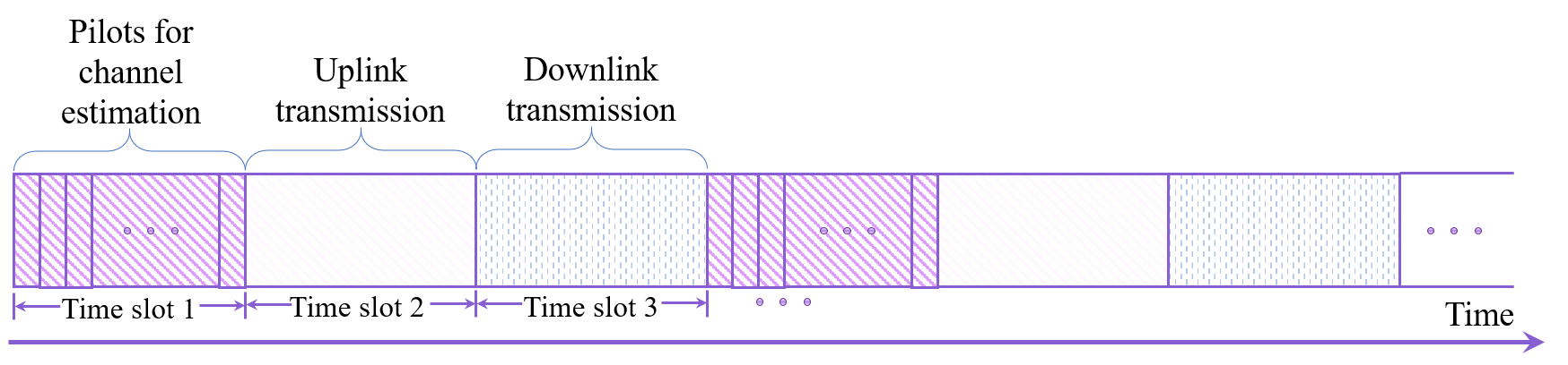
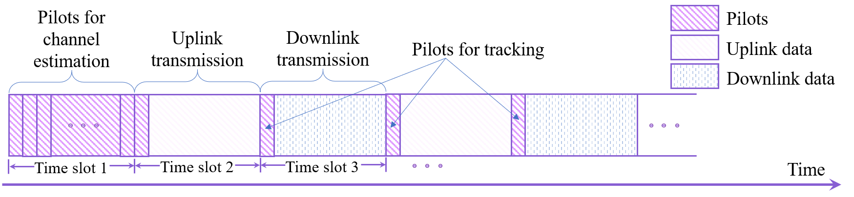
The frame structure for the proposed beamspace multiple-input multiple-output system is similar to the structure in [30], where one total slot is allocated for beamspace channel estimation. Then, assuming that all the user equipments are synchronized, in each time-slot, one pilot is allocated for beam and channel tracking in either uplink or downlink transmissions. Note that the proposed algorithm is also designed to work with only one pilot to update its parameters. The proposed frame structure for the tracking procedure is illustrated in Fig. 2.
III-B Evolution model
In this work, three parameters are considered to track the beam; complex channel coefficients, angle of arrival, and angle of departure. Therefore, in order to prepare the system for tracking, two evolution models should be presented; state and generic models.
In the state-evolution model, the state-space vector for all channel paths at time can be given as
| (8) |
where we separate the channel coefficient into real and imaginary parts to make sure that the angles are real along with the tracking procedures. Since Gauss–Markov model is widely adopted as a simple and effective model to characterize the fading process [31], the evolution model for the channel coefficients can be assumed as a first-order Gauss-Markov [32, 21] given as
| (9) |
where is the channel fading correlation coefficient that characterizes the degree of time variation, and [22]. The generic-evolution model for angle of arrival and angle of departure follows the Gaussian process noise model [20, 21] and given by
| (10) |
with , .
Note that and determines the channel variations. Higher values of and imply fast fading channel, while lower values are used for slow fading channels.
Based on these evolution models, the state-evolution can now be written as
| (11) |
where is a function of the generic-evolution models for complex channel coefficients, angle of arrivals and angle of departures as in (9) and (10). representing the distribution of and with since the channel parameters are considered independent.
III-C Proposed unscented Kalman tracking filter
In this subsection, the proposed unscented Kalman filter algorithm is applied to the system models that described in Section II for beam and channel tracking. unscented Kalman filter is considered as an advantageous to extended Kalman filter due to its ability to adapt to model changes and to overcome the weaknesses of the extended Kalman filter while having the same complexity as explained in [33, 34, 35]. This preference was proved in [36, 37], where the performances of unscented Kalman filter and extended Kalman filter were compared for an autonomous underwater vehicle navigation system. Moreover, unscented Kalman filter is quite suitable for a heavily nonlinear system since its estimation characteristic is not concerned by the level of nonlinearity, which makes the algorithm commonly used in many engineering fields such as integrated navigation [38], autonomous underwater vehicle navigation [36, 37], system identification [39], target tracking [40], and location tracking [41].
In this paper, unscented Kalman filter based algorithm is employed to track the beam. In order to start the tracking, a perfect channel estimation is assumed and the state space vector is initialized from the estimated beam/channel parameters. The input of the proposed algorithm is the state space vector at time represented by its mean and covariance . The measurement/observed symbol is needed as an input to update the algorithm.
The state distribution for the algorithm is represented by a Gaussian random variable specified utilizing a minimal set of carefully chosen sample points. These points are called sigma points and they completely capture the true mean and covariance of and . Noting that when these points propagated through the real-time non-linear system, they can obtain the posterior mean and covariance correctly unlike the extended Kalman filter algorithm where the nonlinearity is approximated to a linear using Jacobian matrix. These sigma points are given as
| (12) | |||
where is the number of state-space elements in and is a scaling parameter such that and it can control the amount sigma points spreading around the mean. These sigma points are then propagated through the process model given in (11) returning in the end a cloud of transformed points . The new estimated mean and covariance are then computed from the transformed points as
| (13) |
| (14) |
where for while and , noting that the weights are normalized to satisfy . is used to incorporate prior knowledge of the distribution of , which is set to 2 as an optimum value for a Gaussian distribution [42], while is a scaling parameter used to identify given that where and are scaling parameters that are responsible of determining the spreading of sigma points around the mean .
The transformed sigma points are then propagated through the nonlinear observation model . Considering the system is tracked in the downlink mode, based on (1), the observation function in a beamspace domain is given as
| (15) |
where is considered as a unit pilot symbols.
For the uplink beamspace transmission, the base station is responsible of tracking multi-beam simultaneously. Therefore, referring to (4), the observation function will lead to multi measurements and is given as
| (16) |
This class of filter can be relevant even when there is a disconnectedness in nonlinear functions and .
The mean and covariance of the transformed observations are measured as
| (17) |
| (18) |
After that, in order to measure the filter gain , the cross covariance between the transformed observation and the transformed sigma points is needed and can be expressed as follow
| (19) |
Therefore, the gain is defined as
| (20) |
Lastly, the posterior state-space vector and its covariance are updated as
| (21) |
| (22) |
The tracking will be repeated for each measurement update on -th time index until the algorithm fails to track due to extreme changes on the channel and new channel parameter estimation is performed.
It should be noted that the algorithm addresses the approximation issues of the extended Kalman filter by using unscented transformation. This concept is generated under the fact that the approximation of a given distribution, by using a fixed number of parameters, is easier than approximating an arbitrary nonlinear function [43]. Following this approach, the unscented transformation obtains a set of sigma points, deterministically chosen as presented in (12). The uniqueness of the unscented Kalman filter algorithm is in the way of selecting these points: numbers, values, and weights. The sigma point method results in a more accurate computation of the nonlinear system tracking where the accuracy is increased as the set of sigma points increases. However, the amount to pay is a significant increase in computational cost as parameters are additionally performed in the system. Therefore, since the spreading of the sigma points can control the accuracy of the unscented Kalman filter algorithm, in this work, the spreading of these sigma points are controlled so that the modified unscented Kalman filter algorithm provides better performance during the tracking time without additional performed parameters.
The effect of different sigma points spreading around the true mean is illustrates in Fig. 3, where it is clearly shown that choosing different spreading can lead to different mean and covariance than the true ones.

In order to optimize the spreading of the sigma points, optimal values for the scaling parameters and are chosen so that the innovation in (21) is minimized, and it is formulated as
| (23) |
The proposed unscented Kalman filter tracking algorithm scheme is summarized in Algorithm 1.


IV Numerical Results
In this section, the numerical results are presented to examine the performance of the proposed tracking algorithm in several scenarios. We explore the impact of different number of user equipments in the system and provide a comparison with extended Kalman filter based tracking algorithm [20, 21]. The performance of each tracking method is shown by calculating the mean square error for the angles which is given as
| (24) |
where is the tracked angles while is the estimated angles considering no tracking is hired in the system. The channel fading correlation for the system is set to be corresponds to slow fading in channel coefficient. A random initialization for the tracking parameters and is given from a uniform distribution , and as a complex standard normal distribution. Due to the similarity in performance for angle of arrival and angle of departure, only the angle of arrival performance is given. It is assumed that the number of radio-frequency chains at base station side is equal to the number of served user equipments in both downlink and uplink transmissions (). Since a reliable high-data transmission in mmWave can be provided with only a few number of path components [44], the downlink and uplink transmissions are assumed to have one path component between each user and the base station during the analysis. As well, based on the sparse nature of the beamspace channel at mmWave frequencies, we can select only a small number of dominant beams to reduce the effective dimension of multiple-input multiple-output system without obvious performance loss. So, few user equipments are served in the system. Each mean square error plot is obtained by averaging over 10000 simulation runs.
IV-A Beam and channel tracking in the downlink transmission
In this subsection, the proposed algorithm is used for tracking at the user side, where the base station can serve multiple user equipments. The system parameters setup is given in Table I.
| Parameters | Value |
|---|---|
| Operating frequency | 28 GHz |
| Channel paths for the tracked user | 1, 5 |
| Channel paths for other user equipments | 1 |
| Antenna array elements at base station | 16 |
| Antenna array elements at all user equipments | 8 |
| Distance between antenna elements | |
| Angle speed variation | , |
| Tracking duration | 20 time slot |
| Channel fading correlation coefficient | 0.99 |
| signal-to-noise ratio | 20 dB |
| Number of user equipments in the system | 1, 4 |
Fig. 4a depicts the mean square error beam tracking performance for single- and multi-user system in the downlink transmission at different speed variation angles. It is seen that as the variation increases from to , the measured error of the proposed tracking algorithm increases from to for single user scenario. Although the proposed algorithm performs poorly when the number of user equipments increases in the system, it can beat the performance of the conventional extended Kalman filter algorithm. It is clearly shown the proposed algorithm outperforms the conventional extended Kalman filter up to 85% performance enhancement in a high speed variation system.
Fig. 4b illustrates the channel tracking performance for both the proposed and the conventional extended Kalman filter algorithms for a single-user system at angle speed variation of . It is noticed that the proposed algorithm gives up to 44% performance enhancement in tracking single path, while it reaches around 66% enhancement for tracking the line-of-sight path and more than 80% for tracking the non-line-of-sight paths in a user that has 5 resolvable channel paths.


IV-B Beam and channel tracking in the uplink transmission
In this subsection, the uplink transmission system is provided where the user equipments are assumed to transmit at same power level and received at the same time by the base station. Note that same power transmission by the user equipments is the worst case scenario due to the high level of inter-user interference observed at the receiver. The proposed algorithm is optimized its parameters according to receiving the user equipments’ signals together. So that all user equipments have been tracked jointly and simultaneously. However, the extended Kalman filter algorithm in this case is employed to track each user channel separately in the presence of receiving signal from other user equipments. The system parameters setup for the uplink transmission are given in Table II.
| Parameters | Value |
|---|---|
| Operating frequency | 28 GHz |
| Channel paths between each user equipment and the base station | 1 |
| Antenna array elements at base station | 16 |
| Antenna array elements at all user equipments | 8 |
| Distance between antenna elements | |
| Angle speed variation for all user equipments | |
| Tracking duration | 20 time slot |
| channel fading correlation coefficient | 0.99 |
| Averaged signal-to-noise ratio from each user equipment | 0 dB |
| Number of user equipments in the system | 1, 2, 4 |
Fig. 5a demonstrates the mean square error performance of angle of arrival beam tracking for the single- and multi-user beamspace multiple-input multiple-output systems while Fig. 5b illustrates the channel tracking performance for the same system at the uplink transmission. According to Fig. 5a, the effectiveness of the proposed algorithm in tracking multiple beams jointly is clearly shown with 62% performance enhancement compared to the conventional extended Kalman filter method. As well, the degradation in performance between different number of user equipments in the system is negligible. However, as shown in Fig. 5b, the performance gap between the proposed algorithm in a single-user system and multi-user system is notable where there is around 90% reduction in performance between one-user system and two-user system. Noting that the gap between the proposed algorithm and the conventional extended Kalman filter based method is increased as well.
V Conclusion
A novel multi-beam joint-tracking algorithm based on unscented Kalman filter filter was designed for multi-user beamspace multiple-input multiple-output systems using lens antenna array. The proposed algorithm is employed to track the channel parameters; angle of arrival, angle of departure, and channel coefficient, of multi-beam jointly. The algorithm avoids Jacobian and/or Hessian matrices computation to provide a linear estimator without any approximation as it is the case in the conventional extended Kalman filter based method. Two implementations were investigated for the beam and channel tracking using the proposed algorithm: 1) single-beam tracking at the user equipment side in the downlink transmission in the presence of other user equipments’ beams interference, and 2) multi-beam joint-tracking at the base station side in the uplink transmission system. Note that the proposed algorithm optimized the sigma points spreading parameters of unscented Kalman filter method which enables us to efficiently track multiple user equipments simultaneously. This leads to enhancing the tracking performance by reducing overall interference in the uplink transmission. The numerical results showed that the proposed algorithm can provide up to 85% performance enhancement in tracking performance compared to conventional extended Kalman filter based method in high mobility systems. The proposed algorithm can be implemented in a highly mobile environment to enhance mobility support by detecting changes in the channel for high-speed users. Also, the proposed algorithm is feasible for devices with limited computation and processing capabilities. As a future work, performance analysis of the presented works can be utilized in a laboratory environment.
Acknowledgement
The work of H. Arslan was supported by the Scientific and Technological Research Council of Turkey under Grant No. 116E078.
Appendix A Analysis of
Given that , , and is equal to
| (25) | |||
Therefore, each element in the matrix can be given as
| (26) |
where and .
Simplifying (26) as
| (27) | |||
where is the Dirichlet sinc function with a maximum of at . It is noticed that each element in is a summation of Dirichlet function with a phase shift of which has the same capabilities of the original Dirichlet sinc function. Therefore, the power in is concentrated only on a small number of elements due to the power-focusing ability of [29].
References
- [1] Z. Pi and F. Khan, “An introduction to millimeter-wave mobile broadband systems,” IEEE Communications Magazine, vol. 49, no. 6, pp. 101–107, 2011.
- [2] R. W. Heath, N. Gonzalez-Prelcic, S. Rangan, W. Roh, and A. M. Sayeed, “An overview of signal processing techniques for millimeter wave MIMO systems,” IEEE Journal of Selected Topics in Signal Processing, vol. 10, no. 3, pp. 436–453, 2016.
- [3] S. Doğan, M. Karabacak, and H. Arslan, “Optimization of antenna beamwidth under blockage impact in millimeter-wave bands,” in 2018 IEEE 29th Annual International Symposium on Personal, Indoor and Mobile Radio Communications (PIMRC). IEEE, 2018, pp. 1–5.
- [4] B. Peköz, M. Hafez, S. Köse, and H. Arslan, “Reducing precoder/channel mismatch and enhancing secrecy in practical MIMO systems using artificial signals,” IEEE Communications Letters, 2020.
- [5] I. Ahmed, H. Khammari, A. Shahid, A. Musa, K. S. Kim, E. De Poorter, and I. Moerman, “A survey on hybrid beamforming techniques in 5G: Architecture and system model perspectives,” IEEE Communications Surveys & Tutorials, vol. 20, no. 4, pp. 3060–3097, 2018.
- [6] A. F. Molisch, V. V. Ratnam, S. Han, Z. Li, S. L. H. Nguyen, L. Li, and K. Haneda, “Hybrid beamforming for massive MIMO: A survey,” IEEE Communications Magazine, vol. 55, no. 9, pp. 134–141, 2017.
- [7] J. Brady, N. Behdad, and A. M. Sayeed, “Beamspace MIMO for millimeter-wave communications: System architecture, modeling, analysis, and measurements,” IEEE Transactions on Antennas and Propagation, vol. 61, no. 7, pp. 3814–3827, 2013.
- [8] Y. Zeng and R. Zhang, “Millimeter wave MIMO with lens antenna array: A new path division multiplexing paradigm,” IEEE Transactions on Communications, vol. 64, no. 4, pp. 1557–1571, 2016.
- [9] M. A. Al-Joumayly and N. Behdad, “Wideband planar microwave lenses using sub-wavelength spatial phase shifters,” IEEE Transactions on Antennas and Propagation, vol. 59, no. 12, pp. 4542–4552, 2011.
- [10] Y. J. Cho, G.-Y. Suk, B. Kim, D. K. Kim, and C.-B. Chae, “RF lens-embedded antenna array for mmWave MIMO: Design and performance,” IEEE Communications Magazine, vol. 56, no. 7, pp. 42–48, 2018.
- [11] O. Quevedo-Teruel, M. Ebrahimpouri, and F. Ghasemifard, “Lens antennas for 5G communications systems,” IEEE Communications Magazine, vol. 56, no. 7, pp. 36–41, 2018.
- [12] Y. Zeng, R. Zhang, and Z. N. Chen, “Electromagnetic lens-focusing antenna enabled massive MIMO: Performance improvement and cost reduction,” IEEE Journal on Selected Areas in Communications, vol. 32, no. 6, pp. 1194–1206, 2014.
- [13] T. Kwon, Y.-G. Lim, B.-W. Min, and C.-B. Chae, “RF lens-embedded massive MIMO systems: Fabrication issues and codebook design,” IEEE Transactions on Microwave Theory and Techniques, vol. 64, no. 7, pp. 2256–2271, 2016.
- [14] P. Y. Lau, Z. N. Chen, and X. Qing, “Electromagnetic field distribution of lens antennas,” in Proc. Asia-Pac. Conference on Antennas Propagation, 2013.
- [15] M. Nazzal, M. A. Aygül, A. Görçin, and H. Arslan, “Dictionary learning-based beamspace channel estimation in millimeter-wave massive MIMO systems with a lens antenna array,” in 2019 15th International Wireless Communications & Mobile Computing Conference (IWCMC). IEEE, 2019, pp. 20–25.
- [16] X. Wei, C. Hu, and L. Dai, “Deep learning for beamspace channel estimation in millimeter-wave massive MIMO systems,” IEEE Transactions on Communications, 2020.
- [17] L. Yang, Y. Zeng, and R. Zhang, “Channel estimation for millimeter-wave MIMO communications with lens antenna arrays,” IEEE Transactions on Vehicular Technology, vol. 67, no. 4, pp. 3239–3251, 2017.
- [18] X. Li, J. Fang, H. Li, and P. Wang, “Millimeter wave channel estimation via exploiting joint sparse and low-rank structures,” IEEE Transactions on Wireless Communications, vol. 17, no. 2, pp. 1123–1133, 2017.
- [19] L. Bai, L. Zhu, J. Liu, J. Choi, and W. Zhang, “Physical layer authentication in wireless communication networks: A survey,” Journal of Communications and Information Networks, vol. 5, no. 3, pp. 237–264, 2020.
- [20] C. Zhang, D. Guo, and P. Fan, “Tracking angles of departure and arrival in a mobile millimeter wave channel,” in Proc. IEEE International Conference on Communications (ICC). IEEE, 2016, pp. 1–6.
- [21] V. Va, H. Vikalo, and R. W. Heath, “Beam tracking for mobile millimeter wave communication systems,” in Proc. IEEE Global Conference on Signal and Information Processing (GlobalSIP). IEEE, 2016, pp. 743–747.
- [22] S. Jayaprakasam, X. Ma, J. W. Choi, and S. Kim, “Robust beam-tracking for mmWave mobile communications,” IEEE Communications Letters, vol. 21, no. 12, pp. 2654–2657, 2017.
- [23] S. Shaham, M. Ding, M. Kokshoorn, Z. Lin, S. Dang, and R. Abbas, “Fast channel estimation and beam tracking for millimeter wave vehicular communications,” IEEE Access, vol. 7, pp. 141 104–141 118, 2019.
- [24] Y. Fan, J. B. Li, H. Li, and C. Tian, “A stochastic framework of millimeter wave signal for mobile users: Experiment, modeling and application in beam tracking,” in Proc. 11th Global Symposium on Millimeter Waves (GSMM). IEEE, 2018, pp. 1–6.
- [25] J. Lim, H.-M. Park, and D. Hong, “Beam tracking under highly nonlinear mobile millimeter-wave channel,” IEEE Communications Letters, vol. 23, no. 3, pp. 450–453, 2019.
- [26] D. Zhu, J. Choi, Q. Cheng, W. Xiao, and R. W. Heath, “High-resolution angle tracking for mobile wideband millimeter-wave systems with antenna array calibration,” IEEE Transactions on Wireless Communications, vol. 17, no. 11, pp. 7173–7189, 2018.
- [27] L. Dai and X. Gao, “Priori-aided channel tracking for millimeter-wave beamspace massive MIMO systems,” in 2016 URSI Asia-Pacific Radio Science Conference (URSI AP-RASC). IEEE, 2016, pp. 1493–1496.
- [28] Z. Wang, M. Li, X. Tian, and Q. Liu, “Iterative hybrid precoder and combiner design for mmWave multiuser MIMO systems,” IEEE Communications Letters, vol. 21, no. 7, pp. 1581–1584, 2017.
- [29] A. Sayeed and N. Behdad, “Continuous aperture phased MIMO: Basic theory and applications,” in 2010 48th Annual Allerton Conference on Communication, Control, and Computing (Allerton). IEEE, 2010, pp. 1196–1203.
- [30] J. Li, Y. Sun, L. Xiao, S. Zhou, and C. E. Koksal, “Fast analog beam tracking in phased antenna arrays: Theory and performance,” arXiv preprint arXiv:1710.07873, 2017.
- [31] M. Medard, “The effect upon channel capacity in wireless communications of perfect and imperfect knowledge of the channel,” IEEE Transactions on Information theory, vol. 46, no. 3, pp. 933–946, 2000.
- [32] J. M. Wooldridge, Introductory econometrics: A modern approach, 6th ed. Nelson Education, 2016.
- [33] S. Lu, L. Cai, L. Ding, and J. Chen, “Two efficient implementation forms of unscented Kalman filter,” in 2007 IEEE International Conference on Control and Automation. IEEE, 2007, pp. 761–764.
- [34] C. Montella, “The Kalman filter and related algorithms: A literature review,” Dec. 2011. [Online]. Available: https://www.researchgate.net/publication/236897001_The_Kalman_Filter_and_Related_Algorithms_A_Literature_Review
- [35] S. Thrun, “Probabilistic robotics,” Communications of the ACM, vol. 45, no. 3, pp. 52–57, 2002.
- [36] B. Allotta, A. Caiti, L. Chisci, R. Costanzi, F. Di Corato, C. Fantacci, D. Fenucci, E. Meli, and A. Ridolfi, “An unscented Kalman filter based navigation algorithm for autonomous underwater vehicles,” Mechatronics, vol. 39, pp. 185–195, 2016.
- [37] B. Allotta, A. Caiti, R. Costanzi, F. Fanelli, D. Fenucci, E. Meli, and A. Ridolfi, “A new AUV navigation system exploiting unscented Kalman filter,” Ocean Engineering, vol. 113, pp. 121–132, 2016.
- [38] Y. Meng, S. Gao, Y. Zhong, G. Hu, and A. Subic, “Covariance matching based adaptive unscented Kalman filter for direct filtering in INS/GNSS integration,” Acta Astronautica, vol. 120, pp. 171–181, 2016.
- [39] A. Kallapur, M. Samal, V. Puttige, S. Anavatti, and M. Garratt, “A UKF-NN framework for system identification of small unmanned aerial vehicles,” in 2008 11th International IEEE Conference on Intelligent Transportation Systems. IEEE, 2008, pp. 1021–1026.
- [40] H. Zhang, G. Dai, J. Sun, and Y. Zhao, “Unscented Kalman filter and its nonlinear application for tracking a moving target,” Optik, vol. 124, no. 20, pp. 4468–4471, oct 2013.
- [41] S. G. Larew and D. J. Love, “Adaptive beam tracking with the unscented Kalman filter for millimeter wave communication,” IEEE Signal Processing Letters, vol. 26, no. 11, pp. 1658–1662, 2019.
- [42] E. A. Wan and R. Van Der Merwe, “The unscented Kalman filter for nonlinear estimation,” in Proc. IEEE Adaptive Systems for Signal Processing, Communications, and Control Symposium. IEEE, 2000, pp. 153–158.
- [43] N. Gordon, B. Ristic, and S. Arulampalam, “Beyond the Kalman filter: Particle filters for tracking applications,” Artech House, London, vol. 830, no. 5, pp. 1–4, 2004.
- [44] S. Han, I. Chih-Lin, Z. Xu, and C. Rowell, “Large-scale antenna systems with hybrid analog and digital beamforming for millimeter wave 5G,” IEEE Communications Magazine, vol. 53, no. 1, pp. 186–194, 2015.