Cluster-based network modeling–automated robust modeling of complex dynamical systems

Cluster-based network modeling is applied to numerous examples, ranging from analytical systems to real-life problems using experimental and simulation data. The main results are summarized in Fig. 4. The first two applications are the Lorenz [26] and Rössler [28] attractors, typical candidates for dynamical systems analysis. The following two implementations are one-dimensional systems: electrocardiogram measurements (ECG) [29], and the dissipative energy from a Kolmogorov flow [30]. The last CNM application is a high-dimensional large eddy simulation of an actuated turbulent boundary layer for skin friction reduction [31].

In this section, we detail the various systems including the numerical setup and the CNM modeling parameters. CNM is fully parametrized by the number of clusters $K$ and the model order $L$. Their selection plays an important role in the model accuracy. The values used for the various systems are listed in Table 1. The procedure to select $K$ and $L$ is detailed in Appendix C. The last column in Table 1 lists the normalized time delays $t_{L}/T_{0}$, where $T_{0}$ is the fundamental period computed from the dominant frequency identified from the autocorrelation function. For purely random signals with no deterministic component, such as the dissipative energy of the Kolmogorov flow, no characteristic period can be defined.

As indicated by the table, the CNM parameters are strongly dependent on the nature of the systems dynamics. Physical interpretation of the chosen parameters is provided for each system in the following.

Robust probability-based data-driven dynamical modeling for complex nonlinear systems has the potential to revolutionize our ability to predict and control these systems. Cluster-based network models (CNM) reproduces the dynamics on a directed network [15], where the nodes are the coarse-grained states of the system. The transition properties between the nodes are based on high-order direct transition probabilities identified from the data. The model methodology is applied to a variety of dynamical systems, from canonical problems such as the Lorenz attractor to rare events to high degrees of freedom systems such as a boundary layer flow simulation. The general methodology is illustrated in Fig. 1 with the Lorenz system and is detailed in the following.

The first step is the data collection, where a set of $M$ states $\bm{x}^{m}$, $m=1,\ldots,M$, also called observations or snapshots, are collected from a dynamical system. They are equally spaced in time by $\Delta t$, so that $\bm{x}^{m}=\bm{x}(m\Delta t)$. There is no restriction regarding the type of system nor the state dimension.

The second step is the identification of the network nodes using an unsupervised clustering algorithm that groups the snapshots into $K$ clusters $\mathcal{C}_{k}$, $k=1,\ldots,K$. In this study, we employ the $k$-means++ algorithm [43, 44, 23] for its simplicity and ability to compute physically meaningful and interpretable centroids. The algorithm performs an iterative search for an optimal centroid distribution that increases the inner-cluster similarity, by executing the following steps:

Step 1:

The initial centroid distribution $\bm{c}_{k}$ is randomly generated.

Step 2:

Each snapshot is affiliated to its closest centroid, following the cluster affiliation function $k$ defined as

$\displaystyle k(\bm{x}^{m})$

$\displaystyle=\text{arg }\underset{i}{\text{min}}\lVert\bm{x}^{m}-\bm{c}_{i}\rVert\,,$

(22)

where $\lVert\bm{x}\rVert=\sqrt{\bm{x}\cdot\bm{x}}$. The function $k$ maps, for each state $\bm{x}^{m}$, the index of the closest centroid.

Step 3:

The inner-cluster variance $J$ of this centroid distribution is computed as

$$J(\bm{c}_{1},\ldots,\bm{c}_{K})=\sum\limits_{k=1}^{K}\sum\limits_{\bm{x}^{m}\in\mathcal{C}_{k}}\lVert\bm{x}^{m}-\bm{c}_{k}\rVert^{2}\,.$$

(23)

Step 4:

The centroid positions are updated by averaging the state snapshots within the corresponding cluster

$$\bm{c}_{k}=\frac{1}{n_{k}}\sum\limits_{\bm{x}^{m}\in\mathcal{C}_{k}}\bm{x}^{m}\,,$$

(24)

where $n_{k}$ is the number of snapshots in cluster $\mathcal{C}_{k}$.

Steps 2 to 4 are repeated until the inner-cluster variance $J$ is minimized below a specified tolerance. Let the vector $\bm{\mathcal{K}}=[\mathcal{K}_{1},\ldots,\mathcal{K}_{I}]$, $\mathcal{K}_{i}\in[1,K]$ contain the indexes of all consecutively visited clusters over the entire time sequence, such that $\mathcal{K}_{i}$ is the index of the $i$th visited cluster. The first and last clusters are $\mathcal{C}_{\mathcal{K}_{1}}$ and $\mathcal{C}_{\mathcal{K}_{I}}$, respectively. The size $I$ of $\mathcal{K}$ is equal to the number of transitions between $K$ centroids over the entire ensemble plus one. The transition time between the sequential clusters is not constant and depends on the state velocity in the phase space. The vector $\bm{\mathcal{K}}$ constitutes the starting point to identify the transition properties between the centroids.

Following the identification of the centroids as the network nodes, the third step of the CNM algorithm characterizes the motion along the nodes. The dynamics are constructed as linear transitions between centroids based on the transition probabilities and the transition times. After a centroid is reached, the next destination is identified using the direct transition probability tensor $\bm{Q}$. The tensor $\bm{Q}$ ignores inner-cluster residence probability and only considers inter-cluster transitions. One novelty of this CNM implementation is to model the direct transition probabilities $\bm{Q}$ using an $L$-order Markov model, which is defined as a conditional probability $\mathrm{Pr}\left(\mathcal{K}_{i}\lvert\mathcal{K}_{i-1},\ldots,\mathcal{K}_{i-L}\right)$. In this context, high-order Markov models are equivalent to time-delay embedding, which are well known in dynamical systems [25]. The benefit of time-delay coordinates is elaborated in Appendix E. For a second-order model, $\bm{Q}\in\mathcal{R}^{K\times K\times K}$ is a third-order tensor and the probability to move to $\mathcal{C}_{l}$, having previously visited $\mathcal{C}_{k}$ and $\mathcal{C}_{j}$, is inferred from the data and given by

$n_{l,k,j}$ designates the number of transitions to $\mathcal{C}_{l}$, having previously visited $\mathcal{C}_{j}$ and $\mathcal{C}_{k}$, and $n_{k,j}$ is the number of transitions departing from $\mathcal{C}_{k}$ coming from $\mathcal{C}_{j}$, regardless of the destination. Note that inner cluster iterations are not possible, by the very definition of a direct transition, such that $Q_{j,j}=\mathrm{Pr}(\mathcal{K}_{i}=j|\mathcal{K}_{i-1}=j)=0$.

The transition time designates the time required to travel from one centroid to the next. In this CNM implementation, the transition time is defined as half of the sum of the residence times in two sequential clusters, as illustrated in Fig. 2 for a first-order model. Let $t^{n}$ and $t^{n+1}$ be the time of the first and last snapshots to enter and, respectively, leave $\mathcal{C}_{k}$ at the $n$th iteration. The iterations designate the sequential jumps between the centroids. The residence time $\tau^{n}$ in $\mathcal{C}_{k}$ is

Following this definition, the individual transition time $\tau_{k,j}^{n}$ from centroid $\bm{c}_{j}$ to centroid $\bm{c}_{k}$ is given by

The transition time $T_{k,j}$ is the average of all transition times $\tau_{k,j}^{n}$ between centroids $\bm{c}_{j}$ and $\bm{c}_{k}$ as

Consistent with the direct transition matrix $\bm{Q}$ for an $L$-order chain, the transition time $\bm{T}$ also depends on the $L-1$ previously-visited centroids.

For large time delays (hence large $L$), the process could yield to two storage-intensive $L+1$-dimensional tensors $Q$ and $T$ with $K^{L+1}$ elements. For instance, clustering with $K=20$ clusters and an order $L=10$, the tensors would contain $20^{11}$ elements, which exceeds the storage capacities of most computers. The expensive tensor creation and storage is circumvented by a lookup table (LUT), where only non-zero entries that correspond to actual transitions are retained. Thus, the tensors are replace by a simple array indexing operation. The look-up tables are typically orders-of-magnitude smaller than the full tensors. As illustration, let’s consider the example in Fig. 1 but with fictional transition properties. Here, all centroids have only one possible destination, except $\bm{c}_{2}$, where the state can transit to either $\bm{c}_{3}$ or $\bm{c}_{5}$ with an assumed equal probability for simplicity ($Q_{3,2,1}=Q_{5,2,1}=0.5$). The 2^nd-order LUT for this example is illustrated in Table 2. The transition times are randomly chosen for this fictional example.

If the state is in $\bm{c}_{2}$ ($k=2$) having visited $\bm{c}_{1}$ before ($j=1$), the next destination is probabilistically chosen between $Q_{3,2,1}$ ans $Q_{5,2,1}$ (lines 5 and 7), yielding a transition to either centroid 3 or centroid 5. If the selected destination is $\bm{c}_{5}$, the corresponding time to this transition is read from $T_{5,2,1}$ (entry # 7).

The fourth and final step of the CNM procedure is state propagation. We assume a linear motion between the centroids. The instantaneous state between two centroids $\bm{c}_{j}$ and $\bm{c}_{k}$ is defined as

where $t_{j}$ is the time when the centroids $\bm{c}_{j}$ is left and $T_{k,j}$ is the transition time from $\bm{c}_{j}$ to $\bm{c}_{k}$. The motion between the centroids may be interpolated with splines for smoother trajectories. As CNM is purely data-driven, the model quality is directly related to that of the training data. More specifically, the sampling frequency and total time range must be selected, such that all relevant dynamics are captured and are statistically converged.

This section presents two metrics used to evaluate the model performance, namely the autocorrelation function and the cluster probability vector. We note the occasional need for additional or different metrics to validate models of certain systems, such as the probability distribution function of a system with rare events.

CNM is parametrized by the number of clusters $K$ and the model order $L$. Both parameters are problem-dependent and can be optimized to achieve the highest prediction accuracy. This section details the current parameters selection process and provides guidelines and recommendations for other datasets.

The number of clusters $K$ determines the resolution level. A small number of clusters will mostly captures the dominant behavior at the macro level, which is suitable for simple dynamics such as a limit cycle. Few centroids also enable easier interpretation of the results and physical insights. Higher $K$ allows to accurately model more complex systems, possibly at the micro scale level, and to uncover a broader range of dynamics including transitional events and higher frequency components. Excessively large $K$ values could be however detrimental, as adjacent trajectories get clustered separately despite describing nearly the same motion. Furthermore, the trajectory of an over-clustered system might introduce an artificial low-amplitude and high frequency noise component resulting from sequential small jumps between misaligned centroids.

The model order $L$ is synonymous with time-delay embeddings in units of past centroids. Increasing $L$ allows modeling of more realistic trajectories, especially when the dynamics have centroids located at the intersections of multiple trajectories, as illustrated in Fig. 8. In this example, trajectory 1 propagates sequentially through centroids $2\to 1\to 3$ and trajectory 2 through centroids $4\to 1\to 5$. With a first-order model, the state at $\bm{c}_{1}$ can possibly transit to $\bm{c}_{3}$ or to $\bm{c}_{5}$, regardless of the previous path. Such a low-order model is thus associated with an increased risk of selecting the wrong trajectory. With a second-order model, however, the previous centroid is taken into account in the conditional probability and the transition from $\bm{c}_{1}$ remains on the correct trajectory, ensuring a more accurate motion. Complex dynamics with multiple intersected trajectories require larger order $L$. For better interpretability, $L$ can be converted into the approximate corresponding time delay $t_{L}$, defined as

where $\overline{T}$ is the overall average transition time.

The values of $K$ and $T$ are problem-dependent. In this work, $K$ and $L$ are selected from a parametric study that minimizes the root mean square error (RMSE) of the autocorrelation function $R(\tau)$ of the reference data and that of the model (see Appendix C for details about $R(\tau)$), defined as

where $\hat{R}$ is the modelled autocorrelation and $N_{R}$ is the maximum lag number. The RMSE distribution for the Lorenz system for varying $K$ and $L$ is presented in Fig. 9A. The results are shown for a range of $K\in[10,100]$, and normalized time delay $t_{L}/T_{0}\in[0.5,1.8]$, where $T_{0}$ is the fundamental period of the system. The black dots denote the computed configurations.

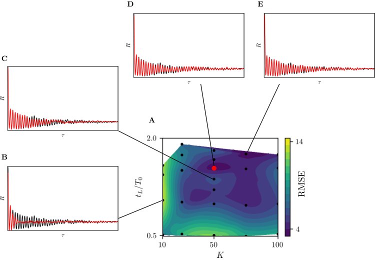
The RMSE does not change linearly with the number of cluster and the model order. The error distribution exhibits regions of high and low error. A low $K$ and low $L$ configuration produces poor dynamics (Fig. 9B), which is expected for a complex system like the Lorenz. As $K$ and $L$ increase, the error generally decreases, despite local maxima (Fig. 9C). The configuration indicated with the red dot (Fig. 9D) is selected for its high accuracy, which is comparable to other more complex models (e.g., Fig. 9E). This winning configuration consists of $K=50$ clusters and an order $L=22$, that corresponds to $t_{L}/T_{0}=1.7$.

The CNM implementation presented in this study builds on two prior cluster-based modeling methods. The first, labelled cluster-based Markov model (CMM), propagates the state using a Markov chain with a constant time step [19]. The second is the initial CNM implementation, which introduced realistic transition times between clusters that yielded a more accurate dynamics [45, 20]. The present work extends CNM to high-order chains for both the transition probability and the transition time. The resulting drastic improvements over the two preceding methods are demonstrated in this section using the Lorenz system as example.

The starting point for CMM and both CNM variants is the clustering of the snapshots into $K$ clusters $\mathcal{C}_{k}$ (for details on the clustering algorithm, see Appendix B). Clustering reduces and coarse-grains the original potentially high-dimensional data into a set of centroids $\bm{c}_{k}$. Both methodologies are described in the main manuscript and are briefly summarized in the following. In CMM, the state variable is $\bm{p}=[p_{1},\ldots,p_{K}]$, where $p_{k}$ is the probability of being in cluster $\mathcal{C}_{k}$. The transition from centroid $\bm{c}_{j}$ to $\bm{c}_{i}$ is guided by the probability transition matrix $\bm{P}=(P_{ij})\in\mathcal{R}^{K\times K}$. The propagation of $\bm{p}$ in time is performed iteratively in steps of $\Delta t$ and is given at time $t^{l}=l\Delta t$ by

The state $\bm{x}$ at time $t^{l}$ is given by

Despite its ability to provide insights into the guiding mechanisms of various physical systems [46, 47], CMM fails at modeling the dynamics. The state vector of cluster probabilities ultimately and unavoidably diffuses to a fixed point representing the post-transient attractor.

The initial CNM version addresses this issue by introducing realistic transition times. At each iteration, the state shifts to a subsequent cluster in a data-inferred time. The direct transition probabilities $\bm{Q}$ and transition times $\bm{T}$ are $K\times K$ zero-diagonal matrices, which result from the state switching centroids at each iteration. The data-inferred transition times drastically increase accuracy compared to CMM, especially for periodic dynamics. This algorithm is, however, not well-suited for complex phase-space trajectories and long time-horizon predictions. The present CNM variant extends the algorithm to high-order Markov models, where both past and current states are jointly considered to determine the next destination cluster and the corresponding transition time. The optimal order is problem-dependent and can be optimized, as detailed in Appendix D. With this latest upgrade, CNM is now capable of modeling any complex nonlinear dynamical system.

The three methods are benchmarked on the Lorenz system, that is described in Appendix A. Clustering is performed with $K=50$ clusters and the model order is set to $L=22$. The cluster probability distribution, which indicates whether the model trajectories populate the phase-space similarly to the data, is depicted for the three methods in Fig. 10A. For clarity of presentation and interpretation, the results are shown for only 10 centroids instead of 50. The coarsening is performed by affiliating the CNM-generated snapshots to the closest of the 10 centroids. The converged probability distribution for CMM matches exactly that of the data, as already reported in the literature [19, 48], whereas those for both CNM variants yield a very good agreement.

The time series of the reference data and of the three models are shown in Fig. 10B to 10E. The reference time series (10B) depict the growing amplitude oscillations in both ears as well as the random ear switching. The CMM temporal evolution in 10C quickly asymptotes toward a fix value after a few oscillations, thus demonstrating the model inability to resolve any meaningful dynamics. Conversely, both CNM models appear to properly duplicate the reference time series (Fig. 10D and Fig. 10E).

The benefits of the high-order CNM become apparent when comparing the autocorrelation function distributions in Fig. 11. As expected, the autocorrelation function from CMM rapidly drops to zero (Fig. 11A). The first-order CNM roughly reproduces the first few iterations, but both amplitude and phase quickly diverge from those of the data (Fig. 11B). In contrast, the high-order CNM, accurately duplicates the oscillations amplitude and phase over the entire range and evidentiates the correct modeling of the dynamics (Fig. 11C).

To disambiguate the effect of internal dynamics from actuation or external input, we generalize CNM to include control $\bm{b}$. This enables predictions beyond the training data for new control parameters $\hat{\bm{b}}$. The main steps of CNMc are illustrated in Fig. 12 and the algorithm is detailed in Algorithm 1.

Before we detail the algorithm, we introduce some the relevant parameters and definitions. Let $I$ be the number of test cases with $I$ different control terms, where the superscript $(i)$ designate the $i$^th test case, $i=1,\ldots,I$. We denote the control term for the new to-be-predicted test case as $\hat{\bm{b}}$. The distance between two control terms $\bm{b}^{i}$ and $\bm{b}^{j}$ is defined by

where $\lVert.\rVert$ designates the Euclidean norm. Similarly to all machine-learning methods, CNMc is inherently limited in its ability to extrapolate beyond the data range. Specifically, the control parameter $\hat{\bm{b}}$ must lie within the range of available control space. Since the method relies on interpolation, two neighboring test cases must be identified. Using the Euclidean distance (40), the two closest operating conditions with the shortest distance to $\hat{\bm{b}}$ are determined. Henceforth, the superscript $(i)$ designates specifically these two neighboring operating conditions, such that $i=1,2$. The snapshots of these two operating conditions are separately grouped into $K$ clusters $\mathcal{C}_{k}^{(i)}$, $k=1,\ldots,K$. Following CNM for individual operating conditions (see Appendix B), the transition probabilities $\bm{Q}^{(i)}$ and transition times $\bm{T}^{(i)}$, of each operating condition are separately computed. For a realistic initialisation of the new to-be-predicted system, the initial state $\hat{\bm{x}}_{0}$ is computed as the average of a centroid from test case ($i=1$) and its nearest neighbor from test case ($i=2$).

Now that the two neighboring test cases are identified, the state of the new test case $\hat{\bm{b}}$ can be propagated. The motion propagation is performed iteratively, following the four steps illustrated in Fig. 12 and detailed in the following.

Step 1:

For each neighboring operating condition $(i)$, the $N_{k}$ closest centroids to the state $\hat{\bm{x}}^{n}$ at iteration $n$ are identified $\bm{c}_{n_{k}}^{(i),n}$, $n_{k}=1,\ldots,N_{k}$. The search is performed using a $k$-d tree, that organizes the data in a tree-like structure to rapidly find nearest neighbors [49]. For low-dimensional data, the $k$-d tree distance metric is typically the Euclidean distance. For the high-dimensional boundary layer data, where the flow is driven by large scale actuation, an alternative norm that reduces high-frequency low-energy small scale contribution is recommended. One possible norm is the $L_{10}$ norm, defined as $\lVert\bm{x}\rVert_{10}=\left(\sum_{i=1}^{n}\lvert x_{i}\rvert^{10}\right)^{1/10}$, which favors the mode coefficients with large magnitude.

Step 2:

The transition properties of the $N_{k}$ nearest centroids are determined. The appropriate $L-1$ past centroids of each neighboring centroid $\bm{c}_{n_{k}}^{(i),n}$ are identified by choosing from all possible trajectories leading to $\bm{c}_{n_{k}}^{(i),n}$ the most similar to the CNMc trajectory, as illustrated in Fig. 13 for a third-order model. In this example, the past centroids of $\bm{c}_{n_{k}}^{(i),n}$ along trajectory 2 are selected, since trajectory 2 is most aligned with $\hat{\bm{x}}$ up to this point. The next centroid $\bm{c}_{n_{k}}^{(i),n+1}$ and the transition time are identified from the corresponding $\bm{Q}$ and $\bm{T}$. The motion direction is based on transition vectors $\bm{v}_{n_{k}}^{(i)}$ that span the transition from $\bm{c}_{n_{k}}^{(i),n}$ to $\bm{c}_{n_{k}}^{(i),n+1}$ as

$$\bm{v}_{n_{k}}^{(i)}=\bm{c}_{n_{k}}^{(i),n+1}-\bm{c}_{n_{k}}^{(i),n}\,.$$

(41)

For the first $L-1$ iterations, the CNMc trajectory is not long enough to identify the $L-1$ past centroids of the neighbors. In that case, the first $L-1$ transition properties are identified from a first-order CNM model.

Step 3:

The transition from $\hat{\bm{x}}^{n}$ to $\hat{\bm{x}}^{n+1}$ is fully characterized by the transition vector $\hat{\bm{v}}$ and the transition time $\hat{T}$, computed by averaging those of the $2N_{k}$ nearest centroids $\bm{c}_{n_{k}}^{(i),n}$. A weighted average can be employed to account for the distance from $\hat{\bm{b}}$ to $\bm{b}^{(1)}$ and $\bm{b}^{(2)}$. In the case where $\hat{\bm{b}}$ is equally distant to $\bm{b}^{(1)}$ and $\bm{b}^{(2)}$, $\hat{T}$ and $\hat{\bm{v}}$ are computed as

	$\displaystyle\hat{T}$	$\displaystyle=\frac{1}{2N_{k}}\sum_{i=1}^{2}\sum_{n_{k}=1}^{N_{k}}T_{n_{k}}^{(i)}\,,$		(42)
	$\displaystyle\hat{\bm{v}}$	$\displaystyle=\frac{1}{2N_{k}}\sum_{i=1}^{2}\sum_{n_{k}=1}^{N_{k}}\bm{v}_{n_{k}}^{(i)}\,.$		(43)

The new position is $\hat{\bm{x}}^{n+1}=\hat{\bm{x}}^{n}+\hat{\bm{v}}$ and is reached in a corresponding time of $t^{n+1}=t^{n}+\hat{T}$.

Step 4:

The optional final step is the position correction. Observations have shown that the predicted dynamics sometimes tend to slide toward one of the two neighboring operating conditions. To circumvent this issue, the position correction forces the state to have a constant relative distance between the two test cases (1) and (2). The distance $d^{(i)}$ between the predicted state $\hat{\bm{x}}$ and a neighboring test case $(i)$ is defined as the distance between $\hat{\bm{x}}$ and the closest snapshot in this test case $\bm{x}^{(i)}$ as

$$d^{(i)}=d\left(\hat{\bm{x}},\bm{x}^{(i)}\right)=\lVert\hat{\bm{x}}-\bm{x}^{(i)}\rVert\,.$$

(44)

The correction is formulated to ensure that the ratio $r$ of the distances between the corrected position $\hat{\bm{x}}_{\text{corr}}^{n+1}$ and the two neighboring test cases is the same as that of the distances between $\hat{\bm{b}}$ and the two neighboring control inputs

$$r=\frac{d\left(\hat{\bm{b}},\bm{b}^{(1)}\right)}{d\left(\hat{\bm{b}},\bm{b}^{(2)}\right)}=\frac{d\left(\hat{\bm{x}}_{\text{corr}}^{n+1},\bm{x}^{(1)}\right)}{d\left(\hat{\bm{x}}_{\text{corr}}^{n+1},\bm{x}^{(2)}\right)}\,.$$

(45)

This is achieved by computing $\hat{\bm{x}}_{\text{corr}}^{n+1}$ as

$$\hat{\bm{x}}_{\text{corr}}^{n+1}=\frac{d_{\bm{b}}^{(2)}\bm{x}^{(1)}+d_{\bm{b}}^{(1)}\bm{x}^{(2)}}{d_{\bm{b}}^{(1)}+d_{\bm{b}}^{(2)}}\,,$$

(46)

where $d_{\bm{b}}^{(i)}=d(\hat{\bm{b}},\bm{b}^{(i)})$ is given by (40).

In addition to the two CNM parameters (number of centroids $K$ and model order $L$), CNMc requires three more settings: The number of closest centroids in each neighboring test case, the norm for the nearest neighbor distance and the optional position correction. These parameters can be optimized for each application separately. One possible approach to optimize these parameters is the hold-out method, where the RMSE is evaluated on the autocorrelation functions. The CNMc parameters for the interpolated Lorenz system and for the boundary layer are summarized in Table 3. The corresponding time series for these two applications are presented in Fig. 14.

References

- [1] P. Holmes, J. L. Lumley, G. Berkooz, C. W. Rowley, Turbulence, coherent structures, dynamical systems and symmetry (Cambridge university press, 2012).
- [2] P. Benner, S. Gugercin, K. Willcox, A survey of projection-based model reduction methods for parametric dynamical systems. SIAM Review 57, 483–531 (2015).
- [3] J. H. Tu, C. W. Rowley, D. M. Luchtenburg, S. L. Brunton, J. N. Kutz, On dynamic mode decomposition: Theory and applications. Journal of Computational Dynamics 1, 391 (2014).
- [4] H. Ye, R. J. Beamish, S. M. Glaser, S. C. Grant, C.-h. Hsieh, L. J. Richards, J. T. Schnute, G. Sugihara, Equation-free mechanistic ecosystem forecasting using empirical dynamic modeling. Proceedings of the National Academy of Sciences 112, E1569–E1576 (2015).
- [5] S. L. Brunton, B. R. Noack, P. Koumoutsakos, Machine learning for fluid mechanics. Ann. Rev. Fluid Mech. 52, 477–508 (2020).
- [6] J. Bongard, H. Lipson, Automated reverse engineering of nonlinear dynamical systems. Proceedings of the National Academy of Sciences 104, 9943–9948 (2007).
- [7] M. Schmidt, H. Lipson, Distilling Free-Form Natural Laws from Experimental Data. Science 324, 81–85 (2009).
- [8] S. L. Brunton, J. L. Proctor, J. N. Kutz, Discovering governing equations from data by sparse identification of nonlinear dynamical systems. Proceedings of the national academy of sciences 113, 3932–3937 (2016).
- [9] F. C. Fu, J. B. Farison, On the Volterra series functional evaluation of the response of non-linear discrete-time systems. International Journal of Control 18, 553–558 (1973).
- [10] C. Chatfield, Time-series forecasting (CRC press, 2000).
- [11] J.-N. Juang, Applied system identification (Prentice-Hall, Inc., 1994).
- [12] T. Wang, H. Gao, J. Qiu, A combined adaptive neural network and nonlinear model predictive control for multirate networked industrial process control. IEEE Transactions on Neural Networks and Learning Systems 27, 416–425 (2016).
- [13] M. Newman, The physics of networks. Physics today 61, 33–38 (2008).
- [14] A.-L. Barabási, R. Albert, Emergence of scaling in random networks. Science 286, 509–512 (1999).
- [15] A.-L. Barabási, E. Bonabeau, Scale-free networks. Scientific American 288, 60–69 (2003).
- [16] J. R. Norris, Markov chains, no. 2 (Cambridge university press, 1998).
- [17] N. Marwan, J. F. Donges, Y. Zou, R. V. Donner, J. Kurths, Complex network approach for recurrence analysis of time series. Physics Letters A 373, 4246–4254 (2009).
- [18] K. Taira, A. G. Nair, S. L. Brunton, Network structure of two-dimensional decaying isotropic turbulence. Journal of Fluid Mechanics 795 (2016).
- [19] E. Kaiser, B. R. Noack, L. Cordier, A. Spohn, M. Segond, M. Abel, G. Daviller, J. Östh, S. Krajnović, R. K. Niven, Cluster-based reduced-order modelling of a mixing layer. Journal of Fluid Mechanics 754, 365–414 (2014).
- [20] H. Li, D. Fernex, R. Semaan, J. Tan, M. Morzyński, B. R. Noack, Cluster-based network model. Journal of Fluid Mechanics (in print), see arXiv:2001.02911 (2020).
- [21] W.-K. Ching, X. Huang, M. K. Ng, T.-K. Siu, Markov Chains: Models, Algorithms and Applications, International Series in Operations Research & Management Science (Springer, 2013), pp. 141–176.
- [22] B. C. Daniels, I. Nemenman, Automated adaptive inference of phenomenological dynamical models. Nature Communications 6, 8133 (2015).
- [23] D. Arthur, S. Vassilvitskii, k-means++: The advantages of careful seeding, Tech. rep., Stanford (2006).
- [24] A. K. Jain, M. N. Murty, P. J. Flynn, Data clustering: a review. ACM Computing Surveys 31, 264–323 (1999).
- [25] F. Takens, Dynamical systems and turbulence, Warwick 1980, Lecture Notes in Mathematics (Springer, University of Warwick, 1981), pp. 366–381.
- [26] E. N. Lorenz, Deterministic Nonperiodic Flow. Journal of the Atmospheric Sciences 20, 130–141 (1963).
- [27] B. Protas, B. R. Noack, J. Östh, Optimal nonlinear eddy viscosity in Galerkin models of turbulent flows. Journal of Fluid Mechanics 766, 337–367 (2015).
- [28] O. E. Rössler, An equation for continuous chaos. Physics Letters A 57, 397–398 (1976).
- [29] S. L. Brunton, B. W. Brunton, J. L. Proctor, E. Kaiser, J. N. Kutz, Chaos as an intermittently forced linear system. Nature Communications 8, 19 (2017).
- [30] M. Farazmand, T. P. Sapsis, A variational approach to probing extreme events in turbulent dynamical systems. Science Advances 3, e1701533 (2017).
- [31] M. Albers, P. S. Meysonnat, D. Fernex, R. Semaan, B. R. Noack, W. Schröder, Drag Reduction and Energy Saving by Spanwise Traveling Transversal Surface Waves for Flat Plate Flow. Flow, Turbulence and Combustion 105, 125–157 (2020).
- [32] Z. Y. Wan, P. Vlachas, P. Koumoutsakos, T. Sapsis, Data-assisted reduced-order modeling of extreme events in complex dynamical systems. PLOS ONE 13, e0197704 (2018).
- [33] G. Van Rossum, F. L. Drake, The python language reference manual (Network Theory Ltd., 2011).
- [34] P. Virtanen, R. Gommers, T. E. Oliphant, M. Haberland, T. Reddy, D. Cournapeau, E. Burovski, P. Peterson, W. Weckesser, J. Bright, S. J. van der Walt, M. Brett, J. Wilson, K. J. Millman, N. Mayorov, A. R. J. Nelson, E. Jones, R. Kern, E. Larson, C. J. Carey, I. Polat, Y. Feng, E. W. Moore, J. VanderPlas, D. Laxalde, J. Perktold, R. Cimrman, I. Henriksen, E. A. Quintero, C. R. Harris, A. M. Archibald, A. H. Ribeiro, F. Pedregosa, P. van Mulbregt, SciPy 1.0: fundamental algorithms for scientific computing in Python. Nature Methods 17, 261–272 (2020).
- [35] A. L. Goldberger, L. A. Amaral, L. Glass, J. M. Hausdorff, P. C. Ivanov, R. G. Mark, J. E. Mietus, G. B. Moody, C. K. Peng, H. E. Stanley, PhysioBank, PhysioToolkit, and PhysioNet: components of a new research resource for complex physiologic signals. Circulation 101, 215–220 (2000).
- [36] E. D. Fylladitakis, Kolmogorov Flow: Seven Decades of History. Journal of Applied Mathematics and Physics 6, 2227–2263 (2018).
- [37] M. Farazmand, T. P. Sapsis, Dynamical indicators for the prediction of bursting phenomena in high-dimensional systems. Physical Review E 94, 032212 (2016).
- [38] D. Bechert, W. Reif, 23rd Aerospace Sciences Meeting (American Institute of Aeronautics and Astronautics, 1985), p. 546.
- [39] M. Luhar, A. S. Sharma, B. J. McKeon, On the design of optimal compliant walls for turbulence control. Journal of Turbulence 17, 787–806 (2016).
- [40] Y. Du, G. E. Karniadakis, Suppressing wall turbulence by means of a transverse traveling wave. Science 288, 1230–1234 (2000).
- [41] M. Quadrio, Drag reduction in turbulent boundary layers by in-plane wall motion. Philosophical Transactions of the Royal Society A: Mathematical, Physical and Engineering Sciences 369, 1428–1442 (2011).
- [42] D. Fernex, R. Semaan, M. Albers, P. S. Meysonnat, W. Schröder, B. R. Noack, Actuation response model from sparse data for wall turbulence drag reduction. Physical Review Fluids 5, 073901 (2020).
- [43] J. MacQueen (University of California, 1967), vol. 1. Conference Name: Proceedings of the Fifth Berkeley Symposium on Mathematical Statistics and Probability.
- [44] S. Lloyd, Least squares quantization in PCM. IEEE Transactions on Information Theory 28, 129–137 (1982). Conference Name: IEEE Transactions on Information Theory.
- [45] D. Fernex, R. Semaan, M. Albers, P. S. Meysonnat, W. Schröder, R. Ishar, E. Kaiser, B. R. Noack, Cluster-based network model for drag reduction mechanisms of an actuated turbulent boundary layer. Proceedings in Applied Mathematics and Mechanics 19 (2019).
- [46] Y. Cao, E. Kaiser, J. Borée, B. R. Noack, L. Thomas, S. Guilain, Cluster-based analysis of cycle-to-cycle variations: application to internal combustion engines. Experiments in Fluids 55, 1837 (2014).
- [47] R. Ishar, E. Kaiser, M. Morzyński, D. Fernex, R. Semaan, M. Albers, P. S. Meysonnat, W. Schröder, B. R. Noack, Metric for attractor overlap. Journal of Fluid Mechanics 874, 720–755 (2019).
- [48] J. Östh, E. Kaiser, S. Krajnović, B. R. Noack, Cluster-based reduced-order modelling of the flow in the wake of a high speed train. Journal of Wind Engineering and Industrial Aerodynamics 145, 327–338 (2015).
- [49] J. L. Bentley, Multidimensional binary search trees used for associative searching. Communications of the ACM 18, 509–517 (1975).