Cosmic evolution in $f(T)$ gravity theory

Since 1998, series of cosmological observations namely TypeIa Supernova Hubble diagram (SNeIa)Riess:1998cb-Perlmutter:1998np, Cosmic microwave background anisotropies (CMBR)Spergel:2003cb, Large Scale Structure (LSS)Tegmark:2003ud and Baryon Acoustic Oscillation (BAO)Eisenstein:2005su predict that our Universe has been undergoing through an accelerated expansion phase. The standard cosmology in the framework of General Relativity (GR) cannot match the overwhelming abundance of the observational evidences of cosmic speedup. One can resolve this paradox by introducing some exotic matter of large negative pressure (known as dark energy (DE)) but difficult questions arise on its nature and introduce further difficult problems. So naturally, cosmologists speculate that these observational evidences may indicate the first signal for the limitation of the Einstein gravity over cosmological scale. As a consequence, there are several modified gravity theories in the literature of which $f(R)$ gravity theory is widely usedCapozziello:2003tk-Carroll:2003wy and gets much attention.

In $f(R)$ gravity theory, the scalar curvature $R$ in the Einstein-Hilbert action is changed to a suitable function $f(R)$. In another modified gravity theory (which is very popular in recent years) known as teleparallel gravity, instead of curvature, torsion represents the gravitational interactionEinstein:1928-Hayashi:1979qx. In fact Einstein first proposed this model to unify electromagnetism and gravity over Weitzenböck non-Riemannian manifold. As a result the Levi-Civita connection is replaced by Weitzenböck connection in the underlying Riemann-Cartan space-time. Hence pure geometric nature of gravitational interaction is no longer there rather torsion acts as a force and one may interpret gravity as a gauge theory of the translation groupArcos:2005ec. It is to be noted that although there are conceptual directions between these two (i.e. GR and teleparallel) gravity theories, still they have equivalent dynamics at least all the classical level.

Further, a generalization to teleparallel gravity (similar to $f(R)$) has been developed Ferraro:2006jd-Harko:2014sjaby replacing torsion scalar $T$ by a generic function $f(T)$. This modified gravity theory is termed as $f(T)$ gravity theory and Linder coined the name. Consequently, there is no equivalence (with GR) at the classical level i.e. distinct dynamics comes into picture. Moreover, there are two important differences between these two theories namely (i) The field equations in $f(T)$ gravity theory remain second order while one has fourth order equations in $f(R)$Bengochea:2008gz, (ii) $f(T)$ gravity theory does not satisfy local Lorentz invariance (which is satisfied by $f(R)$ gravity) so that all 16 components of the vierbien are independent and hence it is not possible to fix six of them by a gauge choiceLi:2010cg. The dynamical object in this model are the four linearly independent vierbein (tetrad) fields which form the orthogonal bases for the tangent space at each point of space-time. The vierbeins are parallel vector fields, which give the theory the descriptor “teleparallel”. The advantage is that the torsion tensor is formed solely from products of first derivatives of the tetrad. This modified teleparallel gravity provides an alternative to inflation Ferraro:2006jd. For details see the review Cai:2015emx-Biswas:2015cva.

In the literature, there are infinite numbers of cosmological solutions describing some of the phases of evolution of the Universe. However, in recent years there are few works Chakraborty:2014oya-Amoros:2013nxa in the literature which describe the whole evolution of the Universe both in Einstein gravity and in some modified gravity theories. In this context the motivation of the present work is 3-fold: (i) to examine whether $f(T)$ gravity theory describes a non-singular model of the Universe, (ii) to show its correspondence with Einstein gravity and (iii) to describe a continuous cosmic evaluation starting from early inflationary era to present accelerating phase with an appropriate continuous choice of $f(T)$. The paper is organized as follows: section II deals with basic equations of $f(T)$ gravity, non-singular (emergent) model of Universe in $f(T)$ gravity has been studied in section III. In section IV correspondence between Einstein gravity and $f(T)$ gravity is presented. Section V contains continuous cosmic evolution in $f(T)$ gravity. The paper ends with a summary in section VI.

The action for $f(T)$ gravity can be written as ($\kappa=8\pi G=1$) Anagnostopoulos:2019miu-Chen:2010va

where $T$ is torsion scalar, $f(T)$ is a differentiable function of torsion, $|e|=\det\left(e^{A}_{\mu}\right)=\sqrt{-g}$, and $L_{m}$ is the matter Lagrangian.

The torsion scalar is defined as

$T_{~\mu\nu}^{\sigma}$, the torsion tensor is defined as

where the Weitzenböck connection $\Gamma^{\sigma}_{\mu\nu}$ is defined as $\Gamma^{\sigma}_{\mu\nu}=e^{\sigma}_{A}\partial_{\nu}e^{A}_{\mu}$ and $S^{~\mu\nu}_{\sigma}$, the super-potential is defined as

In teleparallel gravity, orthogonal tetrad components $e_{A}(x^{\mu})$ are considered as dynamical variables and geometrically they form an orthonormal basis for the tangent space at each point $x^{\mu}$ of the manifold i.e.

Further, in a co-ordinate basis one may write $e_{A}=e^{\mu}_{A}\partial_{\mu}$ where $e^{\mu}_{A}$ are the components of $e_{A}$, with $\mu=0,1,2,3$ and $A=0,1,2,3$. Note that capital letters refer to the tangent space while Greek indices label coordinates on the manifold. Hence the metric tensor is obtained from the dual vierbein as

and $K^{\mu\nu}_{~~\sigma}$, the contortion tensor is given by

In the present work we consider flat, homogeneous and isotropic FLRW (Friedmann-Lemaitre-Robertson-Walker) space-time having line element

where $a(t)$ is scale factor.

Using (2), (3), (4), (5) and (7) one has

where $H=\frac{\dot{a}}{a}$ is the Hubble parameter and overdot represents differentiation with respect to cosmic time $t$. One may note that during cosmic evolution $T$ is negative.

Varying the above action (1) the modified Einstein field equations become

where $f_{T}=\frac{df}{dT}$, $f_{TT}=\frac{d^{2}f}{dT^{2}}$ and $T_{\rho}^{~\nu}$ denotes the total matter (i.e. baryonic and dark energy) energy momentum tensor.

Then for FLRW model the modified Friedmann equations become

where $p$ and $\rho$ are respectively the thermodynamic pressure and density of the matter fluid having the conservation equation

It is to be noted that for various choices of $f(T)$, we have different corresponding gravity theories and it is presented in the following table.

Assuming fluid to be barotropic in nature with equation of state $p=\omega\rho=(\gamma-1)\rho$, $0\leq\gamma\leq 2$ and eliminating $\rho$ from equations (11) and (12), one has the differential equation for cosmic evolution as,

In the context of cosmic evolution the most common idea of the beginning of the Universe is the standard big bang model which evolves from a singularity. To overcome this singularity problem the cosmologists have an idea of emergent scenario of the Universe which is a non-singular model and the cosmological solution represents Einstein static model in infinite past.

In cosmic evolution to have an emergent scenario, the evolution of Hubble parameter have the well known differential equation [Chervon:2014tra,Chakraborty:2014ora,Das:2018bxc]

with parameters $\alpha$ and $\lambda$ are restricted as $\lambda<0$ and $\alpha>|\lambda H_{0}|$ for emergent scenario. Comparing equation (14) with the evolution equation (13) in $f(T)$ cosmology one may choose $f(T)$ as

where $b,~c$ and $d$ are arbitrary constants and hence

where $\beta=\frac{\gamma b\sqrt{6}}{4d}=\gamma\mu,~\mu=\frac{b\sqrt{6}}{4d}.$ Thus this choice of $f(T)$ in equation (15) is purely phenomenological with the motivation of obtaining a solution for emergent scenario.

Depending on the sign of $\beta$ (i.e. $\mu$), one gets various solutions as follows:

If $\beta>0$ (i.e. $\mu>0$), then the cosmological solutions are given by

One may note that equation (III) represents big bang solution for $\beta<3\gamma H_{0}$ (i.e. $\mu<3H_{0}$) while equation (III) represents emergent solution for $\beta>3\gamma H_{0}$ (i.e. $\mu>3H_{0}$) and $\beta=3\gamma H_{0}$ (i.e. $\mu=3H_{0})$ gives the inflationary solution (i.e. the exponential expansion). In particular if one consider

and the cosmological solutions are in the following form

For emergent solution represented by equation (III) one has the following asymptotic behavior

$(i)~a\rightarrow a_{0}2^{-\frac{1}{3\gamma}},H\rightarrow 0~\mbox{as}~t\rightarrow-\infty,$

$(ii)~a\sim a_{0}2^{-\frac{1}{3\gamma}},H\sim 0~\mbox{as}~t\ll t_{0},$

$(iii)~a\sim a_{0}2^{-\frac{1}{3\gamma}}e^{2H_{0}(t-t_{0})},H\sim 2H_{0}~\mbox{as}~t\gg t_{0}.$

Also $\beta=0$ (i.e. $b=0$) and $\beta(=-\nu^{2})<0$ (i.e. $\mu<0$) represent big bang solutions and the solutions are as follows:

and

where $t_{0}$, $a_{0}$, $H_{0}$ and $\rho_{0}$ are integration constants, $a=a_{0}$, $H=H_{0}$, $\rho=\rho_{0}\left(=\sqrt{6}dH_{0}\right)$ at $t=t_{0}$. Hence it is possible to have an emergent scenario of the Universe in $f(T)$ gravity theory. Also the cosmic evolution described above (in equations (III)-(III)) are graphically presented in FIG 1.

The modified Friedmann equations in $f(T)$ gravity given by equations (10) and (11) can be written in the following forms

where $\rho_{e},p_{e}$ are the energy density and thermodynamic pressure of the effective fluid and are given by,

From the field equations (21) and (22) due to Bianchi identity one has,

From equations (12) and (25) one has the individual matter conservation equations as,

Thus the modified Friedmann equations in $f(T)$ gravity can be interpreted as Friedmann equations in Einstein gravity for an non-interacting two fluid system of which one is the usual normal fluid under consideration and other is the effective fluid.

Further using Euler’s thermodynamical equation, the evolution of the temperature of the individual fluid are given by Saha:2014uwa,

Integrating equations (28) and (29) we have,

where $T_{0}$ and $T_{0e}$ are constants of integration. Here $a_{0}$ is the value of the scale factor at the equilibrium era with equilibrium temperature

where $\omega_{0}$ and $\omega_{0e}$ are respectively the values of the equation of state parameters $\omega$ and $\omega_{e}$ at the equilibrium epoch. In particular, using equations (30), the temperature of the normal fluid for constant $\omega$ can be written explicitly in the following form,

In general, at very early phases of the evolution of the universe $T_{e}<T$ and then with the evolution of the Universe $T$ decreases while $T_{e}$ increases and then a state of thermal equilibrium will occur at $T=T_{e}=T_{E}$ at $a=a_{0}$. In the next phase of evolution of universe one has $a>a_{0}$ and $T_{e}>T$ because energy flows from effective fluid to the usual fluid continuously and hence the thermodynamical equilibrium is violated. FIG (2) shows the variation of the temperature $T$ and $T_{e}$ with the scale factor.

Now, from thermodynamical consideration, equilibrium temperature $T_{E}$ can be considered as the (modified) Hawking temperature Chakraborty:2012cw i.e,

where $R_{h}$ is the geometric radius of the horizon, bounding the universe.

Therefore, the present modified gravity theory (i.e. $f(T)$ gravity) is equivalent to Einstein gravity with non-interacting two fluid system having different temperature and the above (modified) Hawking temperature gives the common temperature in equilibrium prescription.

Now after emergent scenario the Universe evolves through three phases, namely, inflationary era, radiation and matter dominated era, and present time accelerating phase. The motivation of this section comes from Chakraborty:2014oya where continuous cosmic evolution has been shown in Einstein gravity with particle creation mechanism. Depending on the choices of the particle creation rate (which are motivated from thermodynamical point of view) it has been shown that there is a continuous cosmic evolution from inflation to the present accelerating era. In this section we shall examine whether such type of continuous cosmic evolution is possible in $f(T)$ cosmology. As there is no physical reason of choosing any form of $f(T)$ so in the following we shall choose $f(T)$ phenomenologically for different eras comparing with the solution equations (in different eras) with that equation (13). Let $t=t_{1}$ and $t=t_{2}(>t_{1})$ be the time instants when the Universe evolves from inflationary era to matter dominated era and then to late time accelerating phase .

For inflationary era ($t<t_{1}$):

Choice for $f(T)$ is

and the cosmological solutions are given by

where $LambertW(x)e^{LambertW(x)}=x$ and $\alpha_{1}$, $\alpha_{2}$, are arbitrary constants.

Here $H_{1}$, $a_{1}$, $\rho_{1}\left(=\frac{\left(6-6\alpha_{2}+\frac{\sqrt{6}\alpha_{1}\mu_{1}}{H_{1}}\right)H_{1}^{2}}{2(\mu_{1}-1)^{2}}\right)$ are the values of the Hubble parameter, scale factor, energy density respectively at $t=t_{1}$, the time instant at which the universe evolves from inflationary era to matter dominated era and $q=-\left(1+\frac{\dot{H}}{H^{2}}\right)$ is the deceleration parameter.

For matter dominated era ($t_{1}<t<t_{2}$):

Choice for $f(T)$ is

and the cosmological solutions are given by

where $\rho_{1}=\frac{\beta_{2}}{2}\left(\frac{\mu_{2}+1}{\mu_{2}-1}\right)\left(6H_{1}^{2}\right)^{\frac{1}{1-\mu_{2}}}$ and $\beta_{1}$, $\beta_{2}$ are arbitrary constants.

For present time accelerating era ($t>t_{2}$)

Choice for $f(T)$ is

and the cosmological solutions are given by

where $H_{2}$, $a_{2}$, $\rho_{2}\left(=3\left(\delta_{2}+1\right)(1-\mu_{2})H_{2}^{2}\right)$ are the values of the Hubble parameter, scale factor, energy density respectively at $t=t_{2}$, the time instant at which the universe makes transition from matter dominated era to the present time accelerating era and $\delta_{1}$, $\delta_{2}$ are arbitrary constants.

Now smoothness of the deceleration parameter demands $\mu_{1}=\mu_{2}$. Also the continuity of the Hubble parameter, scale factor at $t=t_{1}$ is obvious and continuity across $t=t_{2}$ leads to the following conditions

  where

Further, let $t=t_{0}(<t_{1})$ be the time instant in which the universe makes a transition from emergent scenario to inflationary era. Then from the continuity across the transition time $t=t_{0}$, one have

Now, the continuity of $f(T)$ and the energy density across all the transition points $t_{0},~t_{1},~t_{2}$ provides the following conditions

It can be observed that the unknown 8 arbitrary constants: $d,~c,~\alpha_{1},~\alpha_{2},~\beta_{1},~\beta_{2},~\delta_{1},~\delta_{2}$ can be determined by using the equations (40)-(45). So one can easily observe that 2 arbitrary constants must be free. But there are some restrictions on the constants as follows:

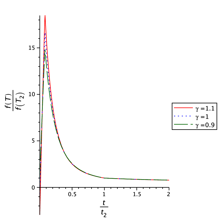
Finally the continuity of $f(T)$ with respect to cosmic time $t$ is also shown graphically in FIG. 3 with the choices $\alpha_{1}=0.3$ and $\alpha_{2}=-0.5$.

A detailed cosmological analysis in $f(T)$ gravity theory has been presented in this work. Firstly, (in section III) it is examined that whether a non-singular model of the universe is possible or not and it is found that for a particular choice of $f(T)$ (given in equation (15)) an emergent scenario is possible only at the level of background cosmology. Note that this choice of $f(T)$ contains terms like square root of $T$ (the $H$ term) and the logarithm of $T$. Hence perturbations must be problematic around emergence of space-time when $T$ tends to zero. Further it is shown that the present $f(T)$ gravity model has a correspondence with the Einstein gravity for non-interacting two fluid system of which one is the usual normal fluid and other is the effective fluid due to the extra geometric term in the $f(T)$ gravity. Also from thermodynamical consideration the temperature of both the fluid particles are evaluated. Lastly, in section V it is possible to have a complete cosmic evolution starting from emergent scenario to present late time accelerating era through the inflationary epoch and matter dominating phase. Hence both physical and geometrical parameters involved in the solutions are found to be continuous (see the figures 1-3) over the entire period of evolution. Therefore, one may conclude that $f(T)$ gravity theory may be considered as an alternative to GR in the context of continuous cosmic evolution as well as to resolve the DE problem.

Last but not least since the model is new in the literature and offers various possibilities including the big bang solution for some choices of the parameters which according to the present observational data is the most preferred cosmological model, thus, it naturally demands further investigations with the available cosmological datasets such as Supernovae Type Ia, Hubble parameter measurements, Baryon Acoustic Oscillations distance measurements etc. This might be very interesting because the constraints on the model parameters will actually indicate the preference of the cosmological scenario explored in this work. We hope to address in a forthcoming work.

The author A.B. acknowledges UGC-JRF (ID:1207/CSIRNETJUNE2019) and S.C. thanks Science and Engineering Research Board (SERB), India for awarding MATRICS Research Grant support (File No.MTR/2017/000407). The authors are also thankful to Dr. Supriya Pan for his valuable comments and suggestions.

References

- (1) A. G. Riess et al. [Supernova Search Team], Astron. J. 116, 1009 (1998).
- (2) S. Perlmutter et al. [Supernova Cosmology Project], Astrophys. J. 517 (1999), 565-586.
- (3) D. N. Spergel et al. [WMAP Collaboration], Astrophys. J. Suppl. 148, 175 (2003).
- (4) M. Tegmark et al. [SDSS Collaboration], Phys. Rev. D 69, 103501 (2004).
- (5) D. J. Eisenstein et al. [SDSS Collaboration], Astrophys. J. 633, 560 (2005).
- (6) S. Capozziello, S. Carloni and A. Troisi, Recent Res. Dev. Astron. Astrophys. 1 (2003), 625.
- (7) S. M. Carroll, V. Duvvuri, M. Trodden and M. S. Turner, Phys. Rev. D 70 (2004), 043528.
- (8) A. Einstein, Sitzungsber. Preuss. Akad. Wiss. Phys. Math. KI. 217 (1928); 401 (1930).
- (9) A. Einstein, Math. Annal. 102 (1930) 685.
- (10) K. Hayashi and T. Shirafuji, Phys. Rev. D 19, 3524 (1979) Addendum: [Phys. Rev. D 24, 3312 (1982)].
- (11) H. I. Arcos and J. G. Pereira, Int. J. Mod. Phys. D 13, 2193 (2004).
- (12) R. Ferraro and F. Fiorini, Phys. Rev. D 75, 084031 (2007), 78, 124019 (2008).
- (13) F. Fiorini and R. Ferraro, Int. J. Mod. Phys. A 24, 1686 (2009).
- (14) E. V. Linder, Phys. Rev. D 81, 127301 (2010) Erratum: [Phys. Rev. D 82, 109902 (2010)].
- (15) A. Finch and J. L. Said, Eur. Phys. J. C 78 (2018) no.7, 560.
- (16) S. Capozziello, O. Luongo, R. Pincak and A. Ravanpak, Gen. Rel. Grav. 50 (2018) no.5, 53.
- (17) S. Basilakos, S. Capozziello, M. De Laurentis, A. Paliathanasis and M. Tsamparlis, Phys. Rev. D 88 (2013), 103526.
- (18) K. Bamba, S. D. Odintsov and D. Sáez-Gómez, Phys. Rev. D 88 (2013), 084042.
- (19) C. Li, Y. Cai, Y. Cai and E. N. Saridakis, JCAP 10 (2018), 001.
- (20) S. Basilakos, S. Nesseris, F. Anagnostopoulos and E. Saridakis, JCAP 08 (2018), 008.
- (21) T. Harko, F. S. N. Lobo, G. Otalora and E. N. Saridakis, Phys. Rev. D 89 (2014), 124036.
- (22) G. R. Bengochea and R. Ferraro, Phys. Rev. D 79, 124019 (2009).
- (23) B. Li, T. P. Sotiriou and J. D. Barrow, Phys. Rev. D 83, 064035 (2011).
- (24) Y. F. Cai, S. Capozziello, M. De Laurentis and E. N. Saridakis, Rept. Prog. Phys. 79, no. 10, 106901 (2016).
- (25) F. Darabi and K. Atazadeh, Phys. Rev. D 100, no. 2, 023546 (2019).
- (26) A. Golovnev and T. Koivisto, JCAP 1811, 012 (2018).
- (27) A. Aviles, A. Bravetti, S. Capozziello and O. Luongo, Phys. Rev. D 87, no. 6, 064025 (2013).
- (28) K. Bamba, M. Jamil, D. Momeni and R. Myrzakulov, Astrophys. Space Sci. 344, 259-267 (2013).
- (29) S. Mishra and S. Chakraborty, Eur. Phys. J. C 79, no. 4, 328 (2019).
- (30) S. K. Biswas and S. Chakraborty, Int. J. Mod. Phys. D 24 (2015) no.07, 1550046.
- (31) S. Chakraborty and S. Saha, Phys. Rev. D 90, no. 12, 123505 (2014).
- (32) D. Das, S. Dutta and S. Chakraborty, Eur. Phys. J. C 78, no. 10, 810 (2018).
- (33) D. Das, S. Dutta and S. Chakraborty, Annals Phys. 397, 410 (2018).
- (34) D. Das, S. Dutta, A. Al Mamon and S. Chakraborty, Eur. Phys. J. C 78, no. 10, 849 (2018).
- (35) M. E. Rodrigues, I. G. Salako, M. J. S. Houndjo and J. Tossa, Int. J. Mod. Phys. D 23, 1450004 (2014).
- (36) E. Elizalde, S. Nojiri, S. D. Odintsov, D. Saez-Gomez and V. Faraoni, Phys. Rev. D 77, 106005 (2008).
- (37) J. Amorós, J. de Haro and S. D. Odintsov, Phys. Rev. D 87, 104037 (2013).
- (38) F. K. Anagnostopoulos, S. Basilakos and E. N. Saridakis, Phys. Rev. D 100, no. 8, 083517 (2019).
- (39) W. El Hanafy and G. G. L. Nashed, Phys. Rev. D 100, no. 8, 083535 (2019).
- (40) Y. F. Cai, M. Khurshudyan and E. N. Saridakis, Astrophys. J. 888 (2020), 62.
- (41) J. Das Mandal and U. Debnath, Adv. High Energy Phys. 2017, 2864784 (2017).
- (42) P. Saha and U. Debnath, Eur. Phys. J. C 76, no. 9, 491 (2016).
- (43) M. U. Farooq, M. Jamil, D. Momeni and R. Myrzakulov, Can. J. Phys. 91, 703 (2013).
- (44) A. V. Astashenok, Astrophys. Space Sci. 351, 377 (2014).
- (45) V. F. Cardone, N. Radicella and S. Camera, Phys. Rev. D 85, 124007 (2012).
- (46) M. Jamil, D. Momeni and R. Myrzakulov, Eur. Phys. J. C 72, 2122 (2012).
- (47) M. Hamani Daouda, M. E. Rodrigues and M. J. S. Houndjo, Eur. Phys. J. C 72, 1893 (2012).
- (48) M. R. Setare and F. Darabi, Gen. Rel. Grav. 44, 2521 (2012).
- (49) T. Wang, Phys. Rev. D 84, 024042 (2011).
- (50) R. Zheng and Q. G. Huang, JCAP 1103, 002 (2011).
- (51) S. H. Chen, J. B. Dent, S. Dutta and E. N. Saridakis, Phys. Rev. D 83, 023508 (2011).
- (52) S. V. Chervon, S. D. Maharaj, A. Beesham and A. S. Kubasov, Grav. Cosmol. 20, 176 (2014)
- (53) S. Chakraborty, Phys. Lett. B 732, 81 (2014)
- (54) S. Pan and S. Chakraborty, Adv. High Energy Phys. 2015, 654025 (2015).
- (55) S. Saha, A. Biswas and S. Chakraborty, Astrophys. Space Sci. 356, no. 1, 141 (2015).
- (56) S. Chakraborty, Phys. Lett. B 718, 276 (2012).