How Does Performance Scale with Antenna Number for Extremely Large-Scale MIMO?

With the fifth-generation (5G) mobile communication networks being deployed worldwide, massive multiple-input multiple-output (MIMO) as a key enabling technology for significantly improving spectral efficiency has become a reality [1]. A typical 5G base station (BS) would be equipped with a massive MIMO array of 64 antenna elements [2]. Looking ahead for beyond 5G (B5G) or sixth-generation (6G) era, there has been growing interest in pushing massive MIMO to another level by further increasing the antenna size/number drastically, for which concepts like ultra-massive MIMO (UM-MIMO), extremely large-scale MIMO (XL-MIMO), and extremely large aperture massive MIMO (xMaMIMO) have been proposed [3, 4, 5, 6].

Compared to existing massive MIMO systems, several new channel characteristics emerge when moving towards XL-MIMO. In particular, the extremely large-scale antenna array at the BS, together with the continuous reduction of cell size, renders the users/scatterers less likely to be located in the far-field region, where conventional uniform plane wave (UPW) assumption is usually made for channel modelling and performance analysis. Note that the typical way for separating far-field versus radiative near-field regions is based on the classical Rayleigh distance ${r_{{\rm{Rayl}}}}=\frac{{2{D^{2}}}}{\lambda}$, where $D$ and $\lambda$ denote the physical dimension of the antenna array and signal wavelength, respectively [7, 8, 9, 10]. More specifically, $r_{\rm{Rayl}}$ corresponds to the minimum link distance so that when the array is used for reception, the maximum phase difference of the received signals across the array elements is no greater than $\frac{\pi}{{\rm{8}}}$ [10, 11]. In the far-field region with the link distance $r\geq r_{\rm{Rayl}}$, the signals can be well approximated as UPW, for which all array elements share identical signal amplitude and angle of arrival/departure (AoA/AoD) for each channel path. However, as the antenna size $D$ further increases so that the users/scatterers are located within the Rayleigh distance, near-field radiation with the more generic spherical wavefront needs to be considered to more accurately model both the signal phase and amplitude variations across array elements. Some preliminary efforts have been devoted towards this direction. In [8], the spherical wave channel under line-of-sight (LoS) conditions was proposed. In [9], the near-field array manifold based on the spherical wavefront model was derived to estimate the location of the near-field source. Apart from the planar and spherical wavefront models, an intermediate parabolic wave model was introduced in [12] to achieve a balance between model accuracy and complexity.

Besides spherical wavefront modelling, another new characteristic of XL-MIMO is the spatial channel non-stationarity in complex propagation environment. Specifically, different regions of the array may observe distinct propagation environment (e.g., different blockers and/or cluster sets), and hence exhibit different levels of received power. One approach for characterizing such spatial non-stationarity is via the concept of visibility region of the array [4, 5, 6, 13].

This paper focuses on the channel modelling and performance analysis of XL-MIMO communication by taking into account the generic spherical wavefront propagation, as opposed to the conventional UPW assumption. To gain useful insights, we first consider the single-user uplink/downlink communication with the optimal maximum ratio combining/transmission (MRC/MRT). A new closed-form expression for the resulting signal-to-noise ratio (SNR) is derived, which generalizes the conventional SNR expression that relies on the simplified UPW assumption. The derived result shows that instead of scaling linearly with the BS antenna number $M$, the resulting SNR based on the more general spherical wavefront model increases with $M$ with diminishing return, governed by a new parameter called angular span, i.e., the angle formed by the two line segments connecting the user with both ends of the antenna array, as illustrated in Fig. 1. Particularly, as $M\to\infty$, the SNR approaches to a constant value that depends on the user’s projected distance to the antenna array. This is in a sharp contrast with the conventional UPW-based result that SNR grows linearly and unbounded with $M$, which is obviously impractical and misleading. One important finding from our derivation is the necessity to introduce a new distance partition criterion, termed critical distance, to complement the classical Rayleigh distance for separating the near- and far-field regions. Different from the Rayleigh distance that is based on the phase difference across array elements and hence depends on the electrical size of the antenna array, the critical distance cares about the amplitude/power difference, which only depends on the physical size of the antenna array. We then extend our study to multi-user XL-MIMO communication, for which we demonstrate that inter-user interference (IUI) can be mitigated not just by angle separation as in conventional multi-antenna systems, but also by distance separation along the same direction. This thus provides a new degree of freedom (DoF) for interference suppression with XL-MIMO. Numerical results are presented to demonstrate the importance of proper spherical wavefront modelling for XL-MIMO communications, by showing the big performance deviation of the conventional UPW-based results from the true values.

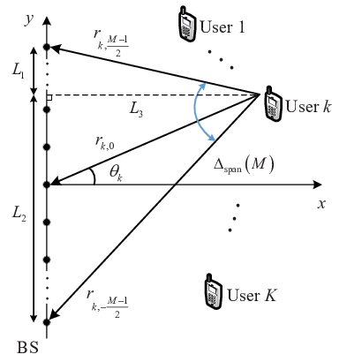
As shown in Fig. 1, we consider a wireless communication system, where a BS with an extremely large-scale antenna array serves $K$ users. For simplicity, we assume that the BS is equipped with an uniform linear array (ULA) with $M\gg 1$ elements, and each user has one single antenna. Without loss of generality, the ULA is placed along the $y$-axis and centered at the origin, and $M$ is an odd number for notational convenience. The location of the $m$th array element is ${{\bf{w}}_{m}}={\left[{0,md}\right]^{T}}$, where $m=0,\pm 1,\cdots,\pm\left({M-1}\right)/2$, and $d\leq\frac{\lambda}{2}$ is the antenna element separation with $\lambda$ denoting the signal wavelength. The location of user $k$ is denoted by ${{\bf{q}}_{k}}={\left[{{r_{k}}\cos{\theta_{k}},{r_{k}}\sin{\theta_{k}}}\right]^{T}},\;1\leq k\leq K$, where ${r_{k}}$ denotes the distance between user $k$ and the center of the antenna array, and $\theta_{k}\in\left[{-\frac{\pi}{2},\frac{\pi}{2}}\right]$ is the angle of the line segment connecting to the user’s location and the array center relative to the $x$-axis. The distance between user $k$ and the $m$th antenna is then given by

where ${\epsilon_{k}}\mathrel{\mathop{\kern 0.0pt=}\limits^{\Delta}}\frac{d}{{{r_{k}}}}$. Note that ${r_{k}}={r_{k,0}}$ and since the array element separation $d$ is on the order of wavelength, in practice, we have $\epsilon_{k}\ll 1$.

By assuming that the communication links between the BS and users are dominated by the LoS component, the array response vector for user $k$ located at distance $r_{k}$ with angle $\theta_{k}$ can be expressed as

where ${a_{m}}\left({{r_{k}},{\theta_{k}}}\right)=\frac{{\sqrt{{\beta_{0}}}}}{{{r_{k,m}}}}{e^{-j\frac{{2\pi}}{\lambda}{r_{k,m}}}}$ with ${\beta_{0}}$ denoting the channel power at the reference distance ${d_{0}}=1$ m. Note that the distance $r_{k,m}$ affects both the amplitude and phase of the array response in (2).

For uplink communication¹¹ 1 Our results can be easily extended to downlink communication., the received signal at the BS can be expressed as

where $P_{k}$ and $s_{k},1\leq k\leq K$ are the transmit power and information-bearing signal of user $k$, respectively; ${\bf{n}}\sim{\cal C}{\cal N}\left({0,{\sigma^{2}}{{\bf{I}}_{M}}}\right)$ is the additive white Gaussian noise (AWGN). With linear receive beamforming ${{\bf{v}}_{k}}\in{{\mathbb{C}}^{M\times 1}}$ applied for user $k$, the resulting signal for user $k$ can be expressed as

The received signal-to-interference-plus-noise ratio (SINR) for user $k$ is then given by

The achievable sum rate in bits/second/Hz (bps/Hz) is

To gain some insights, we first focus on the special case of single-user system, i.e., $K=1$, for which user index $k$ is suppressed in this section. Due to the absence of IUI, it is known that the low-complexity MRC beamformer ${\bf{v}}=\frac{{{\bf{a}}\left({r,\theta}\right)}}{{\left\|{{\bf{a}}\left({r,\theta}\right)}\right\|}}$ is optimal. It follows from (1), (2) and (5) that the resulting SNR can be written as

where $\bar{P}\mathrel{\mathop{\kern 0.0pt=}\limits^{\Delta}}\frac{P}{{{\sigma^{2}}}}$ is the transmit SNR, and $\epsilon=\frac{d}{r}\ll 1$. Note that the subscript ${\left(\cdot\right)_{{\rm{SW}}}}$ signifies that (7) is based on the generic spherical wave channel model as in (2).

Next, we consider the more general multi-user XL-MIMO communications. For simplicity, we focus on the low-complexity MRC receive beamforming with ${{\bf{v}}_{k}}=\frac{{{\bf{a}}\left({{r_{k}},{\theta_{k}}}\right)}}{{\left\|{{\bf{a}}\left({{r_{k}},{\theta_{k}}}\right)}\right\|}}$, $\forall k$, for which the SINR in (5) reduces to

where ${\rho_{ki}}\mathrel{\mathop{\kern 0.0pt=}\limits^{\Delta}}\frac{{{{\left|{{{\bf{a}}^{H}}\left({{r_{k}},{\theta_{k}}}\right){\bf{a}}\left({{r_{i}},{\theta_{i}}}\right)}\right|}^{2}}}}{{{{\left\|{{\bf{a}}\left({{r_{k}},{\theta_{k}}}\right)}\right\|}^{2}}{{\left\|{{\bf{a}}\left({{r_{i}},{\theta_{i}}}\right)}\right\|}^{2}}}}$ denotes the correlation coefficient between user $k$ and $i$. It is noted that different from the conventional modelling based on UPW assumption where the correlation coefficient only depends on the user directions, that for XL-MIMO depends on both the link distances and angle separations.

Fig. 6 shows the correlation coefficient ${\rho_{12}}$ versus the distance separation $\left|{{r_{1}}-{r_{2}}}\right|$ for the conventional UPW and the generic modellings, with the antenna number $M=512$, $1024$, respectively. We assume that user 1 is fixed at ${{\bf{q}}_{\rm{1}}}=\left[{150,0}\right]$ m, and the two user directions are ${\theta_{1}}={\theta_{2}}=0$. It is observed that as the distance separation increases, the correlation coefficient based on the generic modelling decreases in general, as expected, while that based on the conventional modelling is always equal to one. In addition, it is also observed that the increase of antenna number $M$ further helps to reduce the correlation. This implies that the IUI could be mitigated not just by the direction separation as in the conventional UPW modelling, but also by the distance separation along the same direction. Such result shows that there exists a new DoF for interference suppression in XL-MIMO communications.

Fig. 7 shows the sum rate of the multi-user XL-MIMO communication versus the antenna number $M$ with $K=10$ users. We assume that the users are randomly distributed in two areas with area 1 given by ${r_{k}}\in\left[{100,200}\right]$ m, ${\theta_{k}}\in\left[{-\frac{\pi}{4},\frac{\pi}{4}}\right]$, and area 2 ${r_{k}}\in\left[{1000,1200}\right]$ m, ${\theta_{k}}\in\left[{-\frac{\pi}{4},\frac{\pi}{4}}\right]$, $\forall k$. The reference SNR of all users is ${{\bar{P}}_{k}}{\beta_{\rm{0}}}{\rm{=}}\frac{{{P_{k}}{\beta_{\rm{0}}}}}{{{\sigma^{2}}}}=50$ dB, $\forall k$. It is observed that for small $M$, the conventional modelling based on UPW assumption matches with the generic spherical wavefront modelling for both areas considered. Furthermore, for area 2 where users are located far away from the BS, both UPW and the proposed generic modelling give the same results across all $M$ values considered. By contrast, for area 1, with moderately large $M$, the conventional UPW modelling significantly over-estimates the true result. This is due to the fact that with the conventional UPW modelling, each user is treated for having only one single common AoA across all array elements, which thus exaggerates the angle separation for different users when each of them in fact has different AoAs with respect to different array regions for XL-MIMO. As a consequence, the IUI is severely under-estimated with the conventional UPW modelling, and hence the sum rate is over-estimated. This again shows the importance of appropriate spherical wavefront modelling for XL-MIMO communications.

This paper studied the channel modelling and performance analysis of XL-MIMO communication based on the generic spherical wavefront model. For single-user communication with the optimal MRC/MRT beamforming, our newly derived closed-from expression shows that the SNR with the more generic spherical wavefront modelling increases with the antenna number $M$ with diminishing return, governed by a new parameter called angular span. This is in a sharp contrast to the conventional UPW modelling where SNR scales linearly with $M$. Furthermore, we proposed a new distance criterion, termed critical distance, to complement the classical Rayleigh distance for separating the near- and far-field propagation regions. Then for the multi-user XL-MIMO communication system, it was demonstrated that the IUI could be mitigated not just by angle separation as in the conventional modelling, but also by distance separation along the same direction. Numerical results showed the importance of proper spherical wavefront modelling for XL-MIMO communications.

References

- [1] T. L. Marzetta, “Noncooperative cellular wireless with unlimited numbers of base station antennas,” IEEE Trans. Wireless Commun., vol. 9, no. 11, pp. 3590–3600, Nov. 2010.
- [2] J. Zhang, E. Björnson, M. Matthaiou, D. W. K. Ng, H. Yang, and D. J. Love, “Prospective multiple antenna technologies for beyond 5G,” IEEE J. Sel. Areas Commun., vol. 38, no. 8, pp. 1637–1660, Aug. 2020.
- [3] I. F. Akyildiz and J. M. Jornet, “Realizing ultra-massive MIMO (1024 1024) communication in the (0.06–10) terahertz band,” Nano Commun. Netw., vol. 8, pp. 46–54, Jun. 2016.
- [4] E. Björnson, L. Sanguinetti, H. Wymeersch, J. Hoydis, and T. L. Marzetta, “Massive MIMO is a reality – what is next?: Five promising research directions for antenna arrays,” Digit. Signal Process., vol. 94, pp. 3–20, Nov. 2019.
- [5] E. De Carvalho, A. Ali, A. Amiri, M. Angjelichinoski, and R. W. Heath, “Non-stationarities in extra-large scale massive MIMO,” IEEE Wireless Commun., vol. 27, no. 4, pp. 74–80, Aug. 2020.
- [6] A. Amiri, M. Angjelichinoski, E. De Carvalho, and R. W. Heath, “Extremely large aperture massive MIMO: Low complexity receiver architectures,” in Proc. IEEE Globecom Workshops (GC Wkshps), Dec. 2018, pp. 1–6.
- [7] S. Payami and F. Tufvesson, “Channel measurements and analysis for very large array systems at 2.6 GHz,” in Proc. 6th Eur. Conf. Antennas Propag., Mar. 2012, pp. 433–437.
- [8] Z. Zhou, X. Gao, J. Fang, and Z. Chen, “Spherical wave channel and analysis for large linear array in LoS conditions,” in Proc. IEEE Globecom Workshops (GC Wkshps), Dec. 2015, pp. 1–6.
- [9] B. Friedlander, “Localization of signals in the near-field of an antenna array,” IEEE Trans. Signal Process., vol. 67, no. 15, pp. 3885–3893, Aug. 2019.
- [10] C. A. Balanis, Antenna Theory: Analysis and Design. Hoboken, NJ, USA: Wiley, 2016.
- [11] K. T. Selvan and R. Janaswamy, “Fraunhofer and fresnel distances: Unified derivation for aperture antennas,” IEEE Antennas Propag. Mag., vol. 59, no. 4, pp. 12–15, Aug. 2017.
- [12] L. Le Magoarou, A. Le Calvez, and S. Paquelet, “Massive mimo channel estimation taking into account spherical waves,” in Proc. IEEE Int. Workshop Signal Process. Adv. Wireless Commun. (SPAWC), Jul. 2019, pp. 1–5.
- [13] Y. Han, S. Jin, C.-K. Wen, and X. Ma, “Channel estimation for extremely large-scale massive MIMO systems,” IEEE Wireless Commun. Lett., vol. 9, no. 5, pp. 633–637, May 2020.
- [14] I. S. Gradshteyn and I. M. Ryzhik, Table of integrals, series, and products, 7th ed. New York, NY, USA: Academic, 2007.