Centralized active tracking of a Markov chain with unknown dynamics Thanks: Mrigank Raman and Ojal Kumar are with the Mathematics department, and Arpan Chattopadhyay is associated with the EE department and the Bharti School of Telecom Technology and Management, IIT Delhi. Email: {mt1170736, mt1170741 }@maths.iitd.ac.in, arpanc@ee.iitd.ac.in. This work was funded by the PDA and PLN6R budget head, IIT Delhi.
Abstract
In this paper, selection of an active sensor subset for tracking a discrete time, finite state Markov chain having an unknown transition probability matrix (TPM) is considered. A total of sensors are available for making observations of the Markov chain, out of which a subset of sensors are activated each time in order to perform reliable estimation of the process. The trade-off is between activating more sensors to gather more observations for the remote estimation, and restricting sensor usage in order to save energy and bandwidth consumption. The problem is formulated as a constrained minimization problem, where the objective is the long-run averaged mean-squared error (MSE) in estimation, and the constraint is on sensor activation rate. A Lagrangian relaxation of the problem is solved by an artful blending of two tools: Gibbs sampling for MSE minimization and an on-line version of expectation maximization (EM) to estimate the unknown TPM. Finally, the Lagrange multiplier is updated using slower timescale stochastic approximation in order to satisfy the sensor activation rate constraint. The on-line EM algorithm, though adapted from literature, can estimate vector-valued parameters even under time-varying dimension of the sensor observations. Numerical results demonstrate approximately dB better error performance than uniform sensor sampling and comparable error performance (within dB bound) against complete sensor observation. This makes the proposed algorithm amenable to practical implementation.
Index terms— Active tracking, sensor selection, stochastic approximation, Gibbs sampling, on-line expectation maximization.
I Introduction
Remote estimation of physical processes via sensor observations is an integral part of cyber-physical systems. These estimates are typically fed to some controller in order to control a physical process or system. Typical applications of remote estimation include object tracking, environment monitoring, industrial process monitoring and control, state estimation in smart grid, system identification and disaster management. One key challenge is such remote estimation problems is that the sensors are required to perform high-quality sensing, control, communication, and tracking, but they are constrained in terms of energy and bandwidth availability. Hence, it is necessary to activate only the most informative sensor subset at each time, so that a good compromise is achieved between the fidelity of the estimates and energy/bandwidth usage by sensors.
Herein, we consider the problem of designing a low-complexity algorithm for dynamically activating an optimal sensor subset, that minimizes the time-averaged MSE under a sensor activation rate constraint reflecting a constraint on the total energy consumed across sensors. The setup is centralized in the sense that sensors directly report their observations to a remote estimator; in distributed tracking, there can be multiple nodes, each individually estimating a process, via information exchanged over a multi-hop mesh network. In this paper, we consider centralized tracking of a Markov chain with unknown TPM, and solve the problem via a combination of Gibbs sampling, stochastic approximation, and on-line EM. We also work out the problem for the known TPM case. While these algorithms are motivated by solid theoretical consideration, numerical results demonstrate promising MSE performance despite reduced complexity.

I-A Literature survey
Active sensor subset selection for process tracking may be either centralized or distributed. In centralized tracking, sensors send observations to a remote estimator which estimates the process. In distributed tracking, a number of nodes, each having a number of sensors, constitute a connected, multihop network; each node estimates the global state using its local sensor observation and the information coming from the adjacent nodes.
There have been considerable recent work on centralized active tracking of a process with several applications; see [1] for application on sensor networks, [2] for mobile crowdsensing, [3] for body-area sensing application and [4] for target tracking application. Even when the process does not have time-variation, calculating the estimation error given sensor observations and finding the best subset of sensors poses some serious technical challenges. To address these challenges, the authors of [1] provided a lower bound on performance, and used a greedy algorithm for subset selection. On the other hand, there have been a number of recent work on centralized active tracking of a time-varying process: [5] for single sensor selection by a centralized controller to track a Markov chain, Markov decision process formulation for sensor subset selection in [6] to track a Markov chain with known TPM, energy aware active sensing [7], existence and structure of active subset selection policy under linear quadratic Gaussian (LQG) model [8], active sensing for a linear process with unknown Gaussian noise statistics via Thompson sampling [2], etc. The paper [9] considered the model where an observation is shared across multiple sensors. Recently, there have been a series of work for i.i.d. process tracking: [10] using Gibbs sampling based subset selection for an i.i.d. process with known distribution, [11] for learning an unknown parametric distribution of the process via stochastic approximation (see [12]), and an extended version [13] of these two papers. On the other hand, the authors of [14] have proposed an algorithm for distributed tracking a Markov chain with known TPM using tools from stochastic approximation, Gibbs Sampling and Kalman-consensus filter.
I-B Our Contribution
Following points are our contribution in the paper:
- 1.
We provide an online learning algorithm for active sensing to track a Markov chain with unknown TPM. The unknown TPM is learnt via online EM (see [15]), suitably adapted for variable dimension of observations due to active sensing. Gibbs sampling (see [16]) is used for low-complexity sensor activation, and stochastic approximation is used for meeting the sensor activation constraint.
- 2.
An interesting trick to handle variable dimension of observations was to maintain a global library of unknown parameter estimates, and update only the relevant ones in an asynchronous fashion, depending on sensor activation and observation sequence. This idea was absent in the online EM algorithm [15].
- 3.
Another interesting feature of the algorithm which we have proposed is running various iterates in multiple timescales.
I-C Organisation
We have organised our paper in the following manner. In Section II, we have described system model. The necessary mathematical background is summarised in Section III. In Section IV we have provided active sensing, state estimation and learning algorithms. Numerical results are provided in Section V and finally we have conclusion in Section VI.
II System Model
Bold capital and bold small letters will represent matrices and vectors respectively, whereas sets will be represented by calligraphic font throughout this paper.
II-A Sensing and observation model
We consider a remote estimation setting as in Figure 1. The set of sensors is . The sensors are used to sense a discrete time process , which is a time-homogeneous positive recurrent Markov chain with states. For the sake of mathematical convenience, we denote the -th state as which is the -th standard basis (column) vector of length , with at the -th coordinate and everywhere else. Hence, the state space of becomes . The TPM of is denoted by (transpose of ), which is unknown to the remote estimator.
Note that:
| (1) |
where is a zero-mean process noise (non-Gaussian).
At time , let denote the activation status of sensors; if , then the -th sensor is active, otherwise it is inactive. Let be the same as , except that is removed. Also, let be the same as except that , and let us assume similar notation for . An active sensor makes an observation and communicates that observation to the remote estimator, whereas an inactive sensor does neither of these. If and if , then the observation from sensor follows a Gaussian distribution as . Mathematically, we can write the observation coming from sensor at time as:
| (2) |
where is the observation matrix of sensor , and denotes the Gaussian observation noise at sensor . We assume that is independent across sensors and time. We will consider the cases where can be either known or unknown.
The collection of observations , arranged as a column vector via vertical concatenation, is called . This is collected by the remote estimator to estimate at each time . The estimate can be viewed as a belief vector on .
II-B The optimization problem
Let and denote two generic rules (deterministic or randomized) for sensor activation and process estimation, respectively. In this paper, we seek to solve the following problem:
| (3) | |||||
| such that |
By standard Lagrange multiplier theory, problem (3) can be solved by solving the following relaxed problem:
| (4) |
under a suitable Lagrange multiplier such that the inequality constraint is met with equality.
III Background
In this section, we provide a basic background that will be useful in solving (4).
Gibbs sampling: Let us assume (for the sake of illustration) that is i.i.d. with known distribution. Then, there exists an optimal such that, using over the entire time horizon along with MMSE estimation is optimal for (4). Thus, the problem reduces to:
| (5) |
where is the MSE under sensor activation vector , and is the cost under this activation vector. In order to avoid searching over possible activation vectors, the authors of [10] used Gibbs sampling for sensor activation. Gibbs sampling generates a Markov chain whose stationary distribution is with a parameter interpreted as the inverse temperature in statistical physics. Note that, if the unique minimizer for is . Hence, for sufficiently large , Gibbs sampling under steady state selects with high probability, and we obtain a near-optimal solution of (4). At any time , Gibbs sampling randomly selects sensor with uniform distribution, and sets with probability and otherwise. Then the -th sensor is activated accordingly, and the activation status of other sensors remain unchanged. Finally, the constrained problem (3) was solved by using a stochastic approximation (see [12]) iteration , to satisfy the activation constraint.
Expectation maximization: The expectation maximization (EM) algorithm (see [17]) is used to estimate an unknown parameter from noisy observation of a random vector having a parametric distribution with unknown parameter . It maintains an iterate at iteration . In the E step, is computed, and this is maximized over to obtain in the M step. It was shown in [17] that, under certain regularity conditions, converges to the set of stationary points such that . Later, the authors of [15] proposed one online EM algorithm for hidden Markov model; their model is similar to our process and observation models, except that they do not consider active sensing and consider scalar observations of fixed dimension. However, due to active sensing, our problem allows variable dimension of observations, which requires some nontrivial modification of the algorithm of [15].
IV The GEM algorithm
In this section, we propose an algorithm called GEM (Gibbs Expectation Maximization) to solve (3). Since the algorithm is technically involved, we will first describe the major components and concepts related to the algorithm and finally provide a summarised version of the complete algorithm.
IV-A Key components of the algorithm
IV-A1 Some useful notation
| Symbols | Meaning |
|---|---|
| Activation status of sensors | |
| Estimate of the cost of a sensor activation | |
| Running Estimate of Transpose of Transition Probability Matrix | |
| Cost and MSE estimates under activation vector | |
| Running Estimate of mean and covariance of where | |
| Running estimate of the observation matrix | |
| Running estimates of those components of and , that correspond to the active sensors under activation vector |
The proposed algorithm maintains running estimates and for and , respectively. Equivalently, it maintains an estimate of the matrix where . The algorithm also maintains block-diagonal matrices where (block diagonal matrix consisting of these covariance matrix estimates at time ). For an activation vector , we also define another matrix which can be extracted from . Similarly, we define as an estimate of of the column vector (vertical concatenation of these column vectors). Clearly, given and activation vector , our algorithm assumes that . For a given activation vector b we also define the matrix . The algorithm also maintains an estimate for .
The algorithm also maintains the iterates , , and (see Section III), as estimates of , , and , respectively. Estimate of the MSE under activation vector can be denoted by at any time . The quantities are used as cost in Gibbs sampling at time to decide the sensor activation set. The Lagrange multiplier is updated using stochastic approximation so that the activation constraint in (3) satisfies the equality constraint.
We define as the number of times the activation vector is used up to time .
IV-A2 Step sizes
The algorithm maintains two non-increasing, positive step size sequences and for running multi-timescale stochastic approximation updates. The step size sequences satisfy the following properties: (i) , (ii) , (iii) . The first two requirements are standard for stochastic approximation. The third condition is required for timescale separation; the update uses step-size , and the update and online EM updates will use step size .
IV-A3 Gibbs sampling
At time , pick a random sensor uniformly and independently. For sensor , choose = 1 with probability and choose with probability . For all , we choose . Activate sensors according to and obtain the observations .
IV-A4 update
The Lagrange multiplier is updated as:
| (6) |
The iterates are projected onto an interval which is compact namely to ensure boundedness, where is a sufficiently large number. The intuition behind this approach is that, if , then (the cost of a sensor activation) is increased, and is decreased otherwise.
IV-A5 State estimation
We use a Kalman-like state estimator from [6], designed to track a Markov chain. In this algorithm, and denote the estimates of and respectively, given ; here is basically the final estimate declared by the estimator at time , and is an intermediate estimate at time . Additionally, and will denote covariance matrices estimates of the estimation and prediction errors and respectively. Unlike standard Kalman filter where the observation dimension is fixed, this Kalman-like estimator has variable observation dimension depending on , and the gain and error covariance matrix updates also take into account at time .
State Estimation algorithm
Recursion: For each , do:
- 1.
,
(Comment: State estimate at time , keeping observations up to time in account.)
- 2.
,
- 3.
,
(Comment: Estimate of error covariance matrix at time , keeping observations up to time in account.)
- 4.
,
(Comment: Estimate of the observation noise covariance matrix under activation vector , averaged over the belief on the state of the process.)
- 5.
,
(Comment: Kalman gain update.)
- 6.
Compute and project it on the probability simplex.
(Comment: State estimate at time , keeping observations up to time in account. Projection ensures that the estimate is a valid probability belief vector on the state space.)
- 7.
.
(Comment: Estimate of error covariance matrix at time , keeping observations up to time in account.)
IV-A6 update
At time , MSE estimate (for sensor subset only) is updated using the following equation:
| (7) |
IV-A7 Online EM for parameter estimation
Online EM requires an initial distribution for the Markov chain. However, unlike [15], here we have vector-valued observations whose dimension change over time. Also, the unknown parameters and (known and can be handled in a straightforward way) will also have different dimensions for different values of . This requires an asynchronous update of various components of the unknown parameters, depending on the currently active sensors and their observations.
Since the online EM algorithm is heavy in notation, we have made some explanatory comments in between the steps of the algorithm. See [15] for a detailed understanding.
The algorithm requires the auxiliary functions and , and . We also define . In general, we need in the algorithm where ; we define .
Online EM algorithm
Input: Initial distribution of , .
Initialization: Initialize
for all and randomly and compute, for all and ,
,
,
Recursion: For , for all and , DO
Approx. Filter Update
where
(Comment: Here is interpreted as an estimate of the steady state probability distribution of the Markov chain given all observations up to time .)
E-Step
- 1.
- 2.
where .
(Comment: ) and together constitute the expectation of a sufficient statistic for the expected log-likelihood involved in the E step. The sufficient statistic is updated over time using Bayes’ theorem. Details can be found in [15].)
M-Step
- 1.
- 2.
(Comment: Update for the estimate of the transition probability matrix.)
- 3.
- 4.
(Comment: Update for the estimate of the sensor observation mean for subset )
- 5.
(Comment: Update for the estimate of the sensor observation covariance for subset .)
- 6.
For every active sensor such that and for all , modify the values of in and in accordingly.
IV-B The complete algorithm
IV-B1 GEM algorithm
The complete GEM algorithm is outlined below.
The Complete GEM Algorithm
Input: , , , ,
Initialization: Initialise , , , and for all ,
.
Recursion:
For all , DO:
- 1.
Use Gibbs Sampling described in Section IV-A3 to attain , activate sensors accordingly, and collect the corresponding observations .
- 2.
Update as in Section IV-A4.
- 3.
Compute as in Section IV-A5, by running the Kalman-like algorithm.
- 4.
Calculate as in Section IV-A6.
- 5.
Calculate
- 6.
Compute the estimates , and for all , by using online EM as in Section IV-A7.
IV-B2 Discussion
- •
The GEM algorithm runs in multiple timescales (see [12]). Gibbs sampling corresponds to the fastest timescale, and the update and online EM run in the slowest timescale. Timescale separation is ensured by .
- •
update involves asynchronous stochastic approximation for various sensor subsets.
- •
Projection on is done to make sure that all iterates remain bounded.
IV-B3 Computational complexity of GEM for every time
At each time, Gibbs sampling and update require computations. Updating requires computations for trace calculation. The approximate filter update step for all states will require computations due to the matrix inversion involved in calculation. The first step in E step requires computations. Computational complexity of other steps of online EM as well as state estimation is dominated by these two steps and hence the computational complexity of online EM at each time is , where is the dimension of as defined before. The function needs to be computed only for three vectors as required by Gibbs sampling, and hence this requires computations.
V Numerical results
We consider number of sensors , number of states , activation constraint , inverse temperature , , and . The TPM is chosen randomly and then the rows are normalized to obtain a stochastic matrix. The quantities are also chosen randomly. We have not considered larger value of because it is unlikely (even in current cyber-physical systems) that so many sensors estimate a single physical process, especially when the observation from each sensor is a vector.
Under this setting, we compare the performance of the following six algorithms:
- 1.
GEM-K: Here the observation mean and covariances are known (i.e., K), but TPM is unknown.
- 2.
GEM-UK: Here observation covariances are known, but observation mean and TPM are unknown (i.e., UK).
- 3.
GEM-FO: This is GEM Algorithm with full observation. Here all the sensors are always active. The observation mean and covariances are known, but the TPM is unknown.
- 4.
GEM-U: This is GEM Algorithm with uniform random sampling of sensors: at each time , a sensor is activated independently with probability . The observation mean and covariances are known, but the TPM is unknown.
- 5.
GEM-FI: This is GEM with full information of the TPM, observation mean and covariances.
- 6.
GEN: Here GEN stands for genie. At time , the estimator perfectly knows , but no observation is available from sensors. In this case, the MSE will be the limiting variance of given .
V-A Convergence of the algorithms
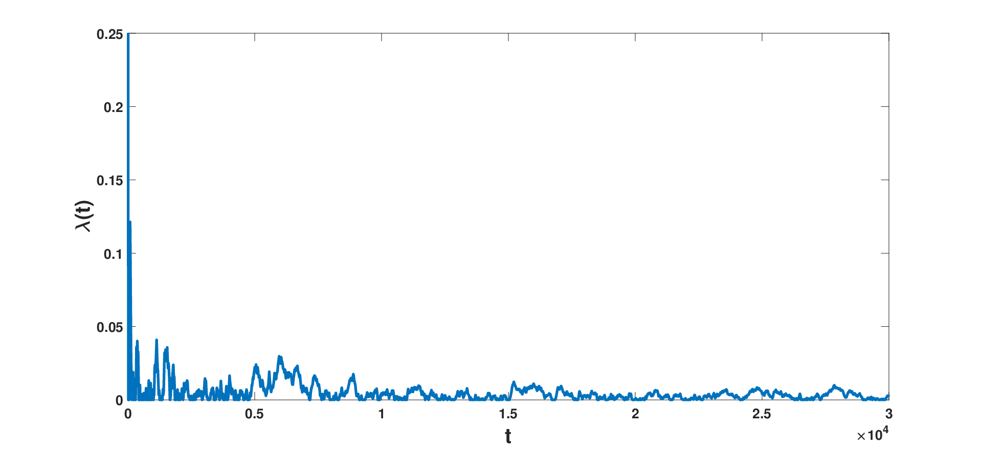
Figure 2 shows the convergence of to for GEM-K. Similarly, we have noticed that converges to for GEM-FO and GEM-U. However, the TPM estimate does not converge to the true TPM for GEM-UK; instead, it converges to some local optimum as guaranteed by the EM algorithm. For all relevant algorithms, we have noticed that the mean number of active sensors, calculated as , converges to ; this has been illustrated only for GEM-K algorithm in Figure 3 and the corresponding variation is shown in Figure 4. We observe that converges at a slower rate.



V-B Performance comparison
In Figure 5, we have compared the MSE performance of various algorithms. We observe that, the TPM estimate in GEM-K converges to the true TPM, and hence the asymptotic MSE performance of GEM-K and GEM-FI are same. Hence, we do not show the MSE performance of GEM-FI separately. Figure 5 shows that, GEN has the best MSE performance due to perfect knowledge of the previous state, and GEM-UK has the worst MSE performance because it converges to a local optimum. GEM-FO performs better than GEM-K because it uses more sensor observation, but it cannot outperform GEN. GEM-U outperforms GEM-UK, since it has knowledge of observation mean and covariances. However, we note in multiple simulations that, on a fair comparison with GEM-K, GEM-U performs worse by approximately dB; this shows the power of Gibbs sampling against uniform sampling.
We have repeated this for different instances, and found that the ordering of MSE performances across algorithms remained unchanged, though the relative performance gaps among the algorithms varied. However, performance gap of GEM-K was observed to be within dB of the MSE of GEM-FO, and within several dB from the MSE of GEN. This shows that GEM is very useful for tracking a Markov chain.
VI Conclusions
We have provided a low-complexity active sensor selection algorithm for centralized tracking of a Markov chain with unknown transition probability matrix. The algorithm uses Gibbs sampling, multi-timescale stochastic approximation, online EM and Kalman-like state estimation to achieve a good compromise among computational complexity, fidelity of estimate, and energy and bandwidth usage in state estimation. Performance of the algorithm has been validated numerically. We seek to prove convergence of the proposed algorithm, and also extend this work for distributed tracking problems in our future research.
References
- [1] D. Wang, J. W. Fisher III, and Q. Liu, “Efficient observation selection in probabilistic graphical models using bayesian lower bounds.”
- [2] F. Schnitzler, J. Yu, and S. Mannor, “Sensor selection for crowdsensing dynamical systems,” in International Conference on Artificial Intelligence and Statistics (AISTATS), 2015, pp. 829–837.
- [3] W. Hui, C. Hyeok-soo, A. Nazim, D. M. Jamal, and H. J. Won-Ki, “Information-based energy efficient sensor selection in wireless body area networks,” in Communications (ICC), 2011 IEEE International Conference on. IEEE, 2011, pp. 1–6.
- [4] F. R. Armaghani, I. Gondal, and J. Kamruzzaman, “Dynamic sensor selection for target tracking in wireless sensor networks,” in Vehicular Technology Conference (VTC Fall), 2011 IEEE. IEEE, 2011, pp. 1–6.
- [5] V. Krishnamurthy and D. Djonin, “Structured threshold policies for dynamic sensor scheduling—a partially observed markov decision process approach,” IEEE Transactions on Signal Processing, vol. 55, no. 10, pp. 4938–4957, 2007.
- [6] D. Zois, M. Levorato, and U. Mitra, “Active classification for pomdps: A kalman-like state estimator,” IEEE Transactions on Signal Processing, vol. 62, no. 23, pp. 6209–6224, 2014.
- [7] ——, “Energy-efficient, heterogeneous sensor selection for physical activity detection in wireless body area networks,” IEEE Transactions on Signal Processing, vol. 61, no. 7, pp. 1581–1594, 2013.
- [8] W. Wu and A. Arapostathis, “Optimal sensor querying: General markovian and lqg models with controlled observations,” IEEE Transactions on Automatic Control, vol. 53, no. 6, pp. 1392–1405, 2008.
- [9] V. Gupta, T. Chung, B. Hassibi, and R. Murray, “On a stochastic sensor selection algorithm with applications in sensor scheduling and sensor coverage,” Automatica, vol. 42, pp. 251–260, 2006.
- [10] A. Chattopadhyay and U. Mitra, “Optimal sensing and data estimation in a large sensor network,” in GLOBECOM 2017-2017 IEEE Global Communications Conference. IEEE, 2017, pp. 1–7.
- [11] ——, “Optimal active sensing for process tracking,” in 2018 IEEE International Symposium on Information Theory (ISIT). IEEE, 2018, pp. 551–555.
- [12] V. S. Borkar, Stochastic approximation: a dynamical systems viewpoint. Cambridge University Press, 2008.
- [13] A. Chattopadhyay and U. Mitra, “Dynamic sensor subset selection for centralized tracking of an iid process,” IEEE Transactions on Signal Processing, 2020.
- [14] ——, “Active sensing for markov chain tracking,” in GlobalSIP 2018. IEEE, 11 2018, pp. 1050—1054.
- [15] O. Cappé, “Online em algorithm for hidden markov models,” Journal of Computational and Graphical Statistics, vol. 20, no. 3, pp. 728–749, 2011.
- [16] P. Brémaud, Markov chains: Gibbs fields, Monte Carlo simulation, and queues. Springer Science & Business Media, 2013, vol. 31.
- [17] B. Hajek, An Exploration of Random Processes for Engineers. Lecture Notes for ECE 534, 2011.