Excitation of gravitational wave modes by a center-of-mass velocity of the sourcePreprint: APS/123-QED
Abstract
Most gravitational wave (GW) sources are moving relative to us. This motion is often closely related to the environment of the source and can thus provide crucial information about the formation of the source and its host. Recently, LIGO and Virgo detected for the first time the subdominant modes of GWs. We show that a motion of the center-of-mass of the source can affect these modes, where the effect is proportional to the velocity of the source. The effect on the GW modes in turn affects the overall frequency of the GW, thus leading to a phase shift. We study the impact of this effect on LIGO/Virgo detections and show that it is detectable for sources with high mass ratios and inclinations. This effect breaks the degeneracy between mass and Doppler shift in GW observations, and opens a new possibility of detecting the motion of a GW source even for constant velocities.
I Introduction
Recently, the LIGO and Virgo detectors detected gravitational waves from merging binary black holes (BBHs) with a significant contribution from modes other than the dominant -mode The LIGO Scientific Collaboration and the Virgo Collaboration 2020a; The LIGO Scientific Collaboration and the Virgo Collaboration 2020b. For the detection of the so-called subdominant modes a relatively high signal-to-noise ratio (SNR) of for the two events as well as significant progresses in modelling waveforms containing subdominant modes accurately have been crucial Khan et al. 2020; Khan et al. 2019; Ossokine et al. 2020; Pan et al. 2014; Babak et al. 2017; Varma et al. 2019. Next-generation ground-based detectors like the Einstein Telescope and Cosmic Explorer Punturo and et al. 2010; Reitze et al. 2019, as well as space-based observatories such as LISA, Tianqin and Taiji Amaro-Seoane et al. 2017; Luo and et al. 2016; Gong et al. 2015 could achieve much higher SNRs of in the future. A higher SNR will then allow us to study subdominant modes in more detail, demanding their modelling to high accuracy.
A feature current GW models have in common is to compute the waveform in a frame where the center-of-mass (CoM) is initially at rest Blanchet 2006; Santamaría et al. 2010; Hannam et al. 2014; Buonanno and Damour 1999; Boyle et al. 2019; Healy et al. 2019; Jani et al. 2016; Blackman et al. 2017. However, the majority of astrophysical objects are constantly moving and hence the templates used by LIGO and Virgo nowadays should be considered as an approximation. This approximations is tolerable for relatively low SNR, but in the future for detections with high SNR, accurate templates should include velocity and its effects on GWs.
Two astrophysical scenarios are of particular interest concerning a CoM velocity of GW sources. The first scenario is the peculiar velocity of galaxies. Other galaxy clusters are moving relative to our Local Group with velocities ranging from about several to around Bahcall 1988; Scrimgeour et al. 2016; Colin et al. 2017. Moreover, a significant fraction of galaxies resides in rich galaxy clusters with velocity dispersions of around Zinn and West 1984; Girardi et al. 1996; Carlberg et al. 1996; Springel et al. 2001; Ruel et al. 2014. Therefore, GW sources from outside of our galaxy can almost always be considered as moving with velocities of several to a few . The second scenario is motivated by the theoretical prediction that a population of merging BBHs may come from triple systems, with the third body being either a star Wen 2003; Naoz 2016; Meiron et al. 2017; Arca Sedda 2020 or a supermassive black hole (BH) in the center of a galaxy Antonini and Perets 2012; McKernan et al. 2012; Addison et al. 2019; Bartos et al. 2017; Stone et al. 2017; Tagawa et al. 2020. The velocities for these systems can range again from a few but go up to several percent of the speed of light Chen et al. 2019; Chen and Han 2018; Han and Chen 2019.
The decomposition of GWs in modes represents a decomposition according to their angular properties, which is conveniently described by the so-called spin-2 spherical harmonics Ruiz et al. 2008; Goldberg et al. 1967. The modes a GW signal contains is not only closely related to the spherical symmetry of the source but also to the multipoles of the source, thus containing detailed information about the structure and dynamics of the source Thorne 1980. In Ref. Torres-Orjuela et al. 2019 we show that the amplitude of a GW signal is velocity-dependent. This change in the amplitude can be explained by the aberration of the GW rays and a rotation of the polarization. These two effects cause that the radiation pattern seen for a moving source differs from the one seen for a source at rest and hence can affect the modes detected for the source. The effect of velocity on the modes of GWs has been studied in the literature for non-relativistic velocities parallel to the line-of-sight, for gravitational kicks and in the context of corrections to Numerical Relativity templates Gualtieri et al. 2008; Boyle 2016; Woodford et al. 2019. In this paper, we study how velocity affects the modes of GWs for general sources and without restriction on the magnitude and orientation of the velocity by focusing on the effects of aberration and polarization rotation on the GWs. We derive how this change results in an excitement of GW modes and study the detectability of this signature by LIGO and Virgo. Throughout this paper, unless otherwise indicated, we use geometrical units in which the gravitational constant and the speed of light are equal to one (i.e., ).
II Gravitational waves modes
In General Relativity, GWs have two independent components, the -polarization, , and the -polarization, , which can be combined to the complex amplitude, . Using this complex amplitude we can decompose the GW in its spherical components, which describe the ‘shape’ of the source, and its time/radial components, which describe the ‘evolution’ of the source. The spherical components are described by spin-weighted spherical harmonics, , of spin Ruiz et al. 2008
| (1) |
The are denoted as the -modes of the GW and are only functions of the time and the radial coordinate. They are defined as
| (2) |
where is the complex conjugate of and represents the integral over the solid angle for .
The spin-weighted spherical harmonics can be explicitly expressed as Goldberg et al. 1967
| (7) |
where
| (8) |
are the binomial coefficients and is the factorial of .
The spin-weighted spherical harmonics fulfill the two following differential properties Ruiz et al. 2008
| (9) | ||||
| (10) |
where and , and the identity
| (11) |
where is the Kronecker-delta. Further, we have for the complex conjugate of a spin-weighted spherical harmonic
| (12) |
III The effect of aberration and polarization rotation on the wave
As shown in Ref. Torres-Orjuela et al. 2019 GWs emitted by a source moving with a constant velocity are affected by aberration and polarization rotation. However, the picture as discussed in Ref. Torres-Orjuela et al. 2019 is not complete. Only the effect of the motion on the the orientation of the wave vector and the polarization directions is considered but not the effect on the modes. The description of the modes is necessary to capture properties of the gradient of the metric, which corresponds to the gravitational field Misner et al. 2017.
Our goal is to describe the modes seen by a distant observer for given modes in the rest frame of the source and a known velocity of the source relative to the observer. For this purpose, we consider how the complex amplitude of a moving source transforms when seen by a distant observer and solve for the modes the resting observer detects. We will see that this transformation and recalculation of the modes induces a mixture of the modes which then in turn affects the evolution of the particular modes.
The transformation of the gravitational radiation at a fixed time can be described by the aforementioned aberration and polarization rotation, when applying them to each ray. In this section, we will derive mathematical expressions for these two effects and then show how they translate into effects on the GW complex amplitude. We use that when considering these effects ray by ray, each ray is only affected by these effects (up to now there is no mode mixture which affects the modes). However, this transformation leads to the complex amplitude being described relative to a non-rectilinear coordinate system (CO) which differs from the one an observer would use. Therefore, when expressing this complex amplitude relative to the CO of the observer we will get a ‘new’ complex amplitude, with modes different from the original ones.
Before deriving how aberration and polarization rotation affect the complex amplitude, let us establish appropriate COs. The decomposition in spin-weighted spherical harmonics is usually performed around the source. Therefore, we set a CO attached to the source’s CoM so that the -axis is perpendicular to the orbital plain and the - and -axes lie in the orbital plain. We denote the polar angle, measured relative to the -coordinate, by and the azimuthal angle, measured from the -coordinate, by . Moreover, we consider an observer far enough from the source so that the space-time around him is flat except for the GWs and assume the CoM of the source to be moving with a velocity relative to this observer. As shown in Ref. Boyle 2016, a rotation of the coordinate system can affect the modes but in a different manner as a velocity. Therefore, for simplicity and without restriction of generality, we set the COs of the observers or to be parallel to the COs of the source in the limit of vanishing velocity.
Last, we would like to mention that in the case of a time-dependent motion, more effects than aberration and polarization rotation can appear (see, e.g., Ref. Torres-Orjuela et al. 2020 for a time-dependent phase shift induced by aberration) but, for simplicity, we do not consider them and focus on the effects of a constant velocity.
III.1 Aberration
Like for light, the velocity of GWs is finite but equal for all observers. Therefore, for an observer the same GW ray points in different directions when the source is moving as when the source is at rest. This effect, known as ‘aberration’ for light Jackson 1999, changes the perceived shape of a GW source and thus its decomposition in modes.
In the observer and the source frames the direction vectors (the spatial parts of the wave vector) of a GW ray can be described, respectively, by the radial vectors and , respectively. Using a Lorentz transformation and normalizing the resulting vector, we find that the two vectors are related by Torres-Orjuela et al. 2020
| (13) |
where is the Lorentz factor and is the three dimensional Euclidean scalar product.
The aberration of the ray makes that the direction vector pointing towards in the observer frame points towards in the source frame. The angles in the source frame can be computed using the direction vector, , as
| (14) | ||||
| (15) |
where and . Note that and are functions of the spherical coordinates because of the projection of the velocity vector, , on the radial vector, .
III.2 Polarization rotation
The geometry of GWs is described by the aforementioned direction vector and the directions of the polarizations. The latter are represented by two spatial vectors of unit length that are perpendicular to each other and the direction vector. Lorentz transformations do not preserve angles in space. Therefore, the directions of the polarizations do not transform according to a Lorentz transformation between a moving source and one at rest Thorne 1987. Their proper transformation is shown in Eqs. (16) and (17) and in fact induces a rotation of the directions of the polarizations in the plane perpendicular to the direction vector. Such a rotation will also affect the spherical properties of the GWs.
In the observer frame the directions of the polarizations can be represented by the two spatial 4-vectors and . For a source moving with a 3-velocity , or accordingly a 4-velocity , the directions of the polarizations have the form Thorne 1987
| (16) | ||||
| (17) |
Here is the Minkowsky product, is the normalized wave vector and is the time vector. Note that and do not differ from and , respectively, by a Lorentz transformation but through a transformation imposed by their basic properties. The polarization rotation is then the angle by which is rotated relative to , i.e., the Lorentz transformed polarization directions, in the plane perpendicular to the GW direction vector. Note that transform like contravariant vectors because they are the basis of the GW tensor.
The and are all perpendicular to the 4-velocity, , and hence spatial vectors in the source frame. Moreover, they are all vectors of unit length. Therefore, and as well as and can only differ from each other by spatial rotations
| (18) | |||
| (19) |
where is a rotation by an angle along the vector for .
The are related to rotations due to the aberration. Therefore, we focus on the , which represent the rotations of the polarization in the plane perpendicular to the direction vector. Using that and are all spatial vectors of unit length we get that and . Using that for purely spatial vectors and , we find
| (20) | ||||
| (21) |
In particular, we find that both vectors are rotated by the same angle , which is what we expect for a rotation of the polarization that preserves its properties. Note that because of the projection of the velocity, , on the coordinate vectors, , the rotation angle is a function of the spherical coordinates, .
III.3 The effect on the complex amplitude of the wave
Aberration and polarization rotation affect the complex amplitude of the wave. Therefore, for a distant observer a GW source moving appears different from one at rest. In this section we relate the complex amplitude of a moving source seen by a distant observer, , to the complex amplitude of the source in its own rest frame, .
The complex amplitude is a function of the spherical coordinates. Therefore, aberration causes that the observer sees the complex amplitude as
| (22) |
where denotes the transformation of the spherical coordinates induced by aberration and described in Eqs. (14) and (15). We, further, note that the transformation is itself a function of the spherical coordinates and hence cannot be described by a global transformation of the CO.
We know that GWs are not only affected by aberration but also by polarization rotation. A rotation of the basis vectors of the polarization in the same plane by an angle (cf. Eq. (20)). This rotation means the polarizations combine to form ‘new’ polarizations
| (23) | ||||
| (24) |
Using Euler’s equation, we then find for the complex amplitude
| (25) |
where . Note that because the polarization rotation is a function of the spherical coordinates, too, it cannot be described by a global transformation of the CO and, in particular, the phase shift does not represent a constant phase shift.
We find that the complex amplitude of the moving source transforms to the CO of the distant observer in a way that depends on the spherical coordinates . Therefore, the decomposition in spherical modes of the moving source in the observer’s rest frame differs from the decomposition in its own rest frame. We will elaborate this step in the next section.
IV Excitation of the modes
The modes of GWs represent the decomposition of the wave according to its spherical properties. A motion of the CoM of the source can affect the shape of the source through aberration and polarization rotation, as depicted in Fig. 1, thus changing these modes. In this section we show how the GW modes apparent to an observer change with the velocity of the source.
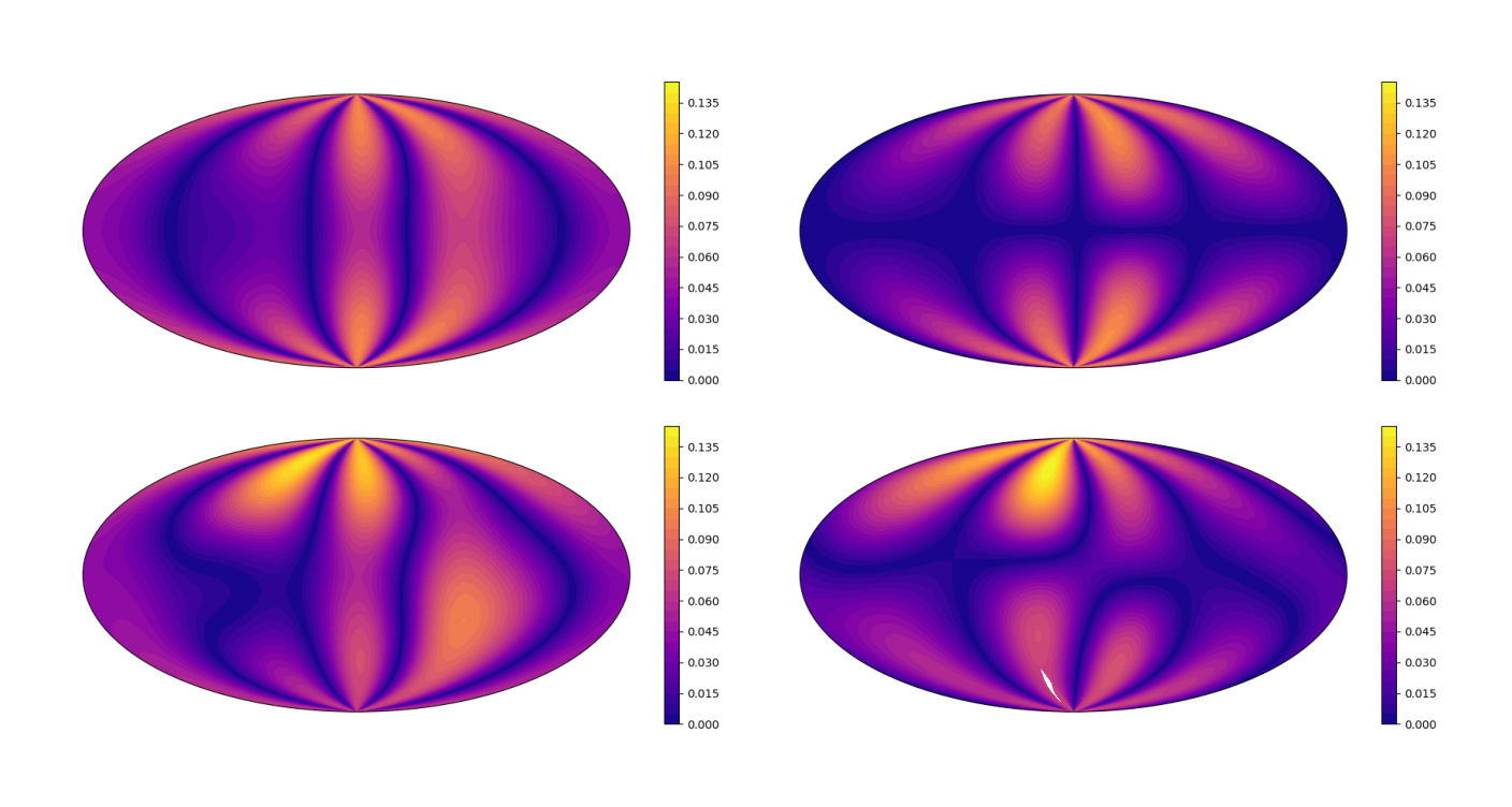
For the complex amplitude of the moving source as seen by the observer, we have
| (26) |
where means the transformations due to polarization rotation and aberration combined. Our goal is to derive explicit expressions for the modes of the moving source, , in terms of the modes of the source at rest, , and the velocity of the source, , up to leading order in the amplitude of the velocity, . Such an expansion is physically well motivated, since we expect most of the sources to have CoM velocities much smaller than the speed of light.
We start by expanding Eq. (26) using the coordinates . We only will replace the primed coordinates by the observer’s coordinates, , after the expansion, to simplify the notation. However, this is just a matter of notation and does not place a restriction on the results. After expanding, we get
| (27) |
Using that , and , we get
| (28) |
From Eq. (20) we see that the rotation of the polarization only enters to the third order of and hence we can ignore the last term in the previous equation. We, further, replace and using Eqs. (14) and (15) and expand again to linear order in , to find
| (29) |
where .
Using the decomposition of in terms of spin-weighted spherical harmonics in Eq. (1) and the differential properties in Eqs. (9) and (10), we then find
| (30) |
where
| (31) |
and
| (32) |
The are functions of the spherical coordinates. Therefore, we need to further decompose Eq. (30) in order to get expressions in terms of only the spin-2 spherical harmonics and functions of only the time and radial coordinates. We decompose in terms of spin-2 spherical harmonics, thus finding
| (33) |
where
| (34) |
Using Eqs. (11) and (12), we then get
| (35) |
The integral in Eq. (IV) can be solved analytically using the expression in Eq. (II) and by decomposing it in its partial integrals, to find
| (36) |
Explicit expressions for , and can be found in the appendix.
A remarkable feature in Eq. (IV) is that a mode from a moving source of the order only has contributions from the modes of a source at rest of the orders , and but of all orders . We expect contributions from modes of the orders when including terms of the order . However, why the the order scales with the order of the velocity, while the order is independent of the order of the velocity, remains a question that requires further analysis.
We point out that the approach we use here implicitly assumes a decomposition of GWs in their modes at a fixed time, since we consider the effects of velocity on the direction vector and the polarization vectors but not on the frequency. The frequency of GWs is affected by a velocity through Doppler shift, which is also direction-dependent and hence could affect the decomposition of GWs in modes. However, to consider the effect on the frequency would require to account for an evolution in time, which lies beyond the scope of this work. To detect the change in the evolution, an observation period of the order of , where is the frequency of the GW and is the maximal difference in the frequency induced by the Doppler shift, is needed, which for typical velocities ( the speed of light) is of the order of several hundred cycles and hence much longer than the typical duration of a LIGO/Virgo event The LIGO Scientific Collaboration and the Virgo Collaboration 2019; The LIGO Scientific Collaboration and the Virgo Collaboration 2021. Therefore, our approach represents an important step in understanding the effect of velocity on the modes of GWs but more work considering the Doppler shift needs to be conducted in order to obtain a more complete picture. Despite the restrictions of our approach, we will analyse in the remainder of this paper the consequences of our results for GWs taking into account their evolution in time. Although, the results obtained may not represent the complete picture they are still valid and can be considered as a minimal case. In particular, we expect that by considering the Doppler effect the modes from a moving source and one at rest will differ even more.
In Fig. 2 we compare the polarizations of a moving source, , and those of a source at rest, . In the upper plot we see that the amplitude of the -polarization for the moving source is enhanced relative to the amplitude of the source at rest. However, in the lower plot we see that for the -polarization the amplitude of the moving source is suppressed relative to the amplitude of the non-moving source. Note, that this is not a general feature but depends on the specific properties of the source, the velocity and the viewing angle. Moreover, the frequency of the GWs from the moving source is shifted by a time-dependent factor relative to the frequency of the GWs from the source at rest. This shift appears because the overall frequency of GWs depends on the relative contribution of the particular modes, which for a moving source is different from one at rest. We discuss this effect in more detail in Sec. VI.
V Breaking the degeneracy between Doppler shift and mass
It is well known that, when only considering the effect of motion on the frequency of GWs, a moving source is degenerate with a source with identical parameters but with a different mass Schutz 1986; Cutler and Flanagan 1994. This circumstance is usually denoted as the mass-redshift degeneracy of GWs. However, in the previous section we showed that when considering aberration and polarization rotation, not only the frequency of the GWs changes but also the amplitude of their spherical modes. This change of the modes leads to a change in the amplitude of the polarizations and a time-dependent frequency shift, which makes it possible to differ between a moving source and one at rest.
One now might think that a moving source and one at rest remain degenerate if one not only adjust their mass to account for the Doppler shift but also their orientation to account for the effects of aberration and polarization rotation. In this section we show this is not true. That means we show that the GWs from a moving source differ from those from a source at rest, regardless of any variation of the mass and orientation.
To show the difference between the resting and the moving source, we consider two sources with identical properties but the source at rest having a mass and the moving source a mass . Here, is the Doppler shift in direction and its correction ensures that the time scales of both systems are the same in the frame of a distant observer. If the source at rest and the moving one indeed only would differ by an additional correction of their orientation, we would have
| (37) |
where are two smooth functions of and the velocity of the source. By showing that this equation is not true, we will prove that the two sources have different signals.
We start using the mode decomposition of the two complex amplitudes in Eq. (37), multiplying the equation by and integrating over , to get
| (38) |
Because are smooth functions of , can be decomposed in terms of spin-2 spherical harmonics over the basis
| (39) |
where
| (40) |
Using this decomposition and Eq. (11), we find
| (41) |
Last, we replace using Eq. (IV) and get
| (42) |
We see that on the left hand side of this equation the index is independent of the modes of the source, . In contrast on the right hand side the index depends on the modes of the source for all four terms. Therefore, for general sources and velocities Eq. (V) is not fulfilled.
To make this more clear, we consider a hypothetical source with only the mode. In this case Eq. (V) reduces to the form
| (43) |
Here, the left hand side depends on through the while the right hand side, in contrast, is independent of . Therefore, for Eq. (V) to be fulfilled it would be necessary that the are independent of . For that to happen would require that the velocity has no components perpendicular to the angular momentum of the source so that it is independent of . However, for general sources and orientations of the velocity this is not true, thus implying that Eq. (V) is in general not fulfilled. We note that the velocity being parallel to the angular momentum of the source is necessary but not sufficient to ensure that Eq. (V) is fulfilled. Even in the case where the velocity has no components perpendicular to the angular momentum of the source the can depend on .
We have shown that the GWs from two sources with the same properties, except that one is moving and the other at rest, and a correction of their masses to account for the Doppler shift, look different. This remains true even when assuming the observer can ‘adjust’ the orientation of the two sources. Thereby we have proven that for moving sources the degeneracy between mass and Doppler shift can be broken when considering the higher modes of the source.
Note, that for our proof we assumed to have two sources with identical properties except for their velocity and mass. To detect the velocity with certainty would, however, require to extract the effect of the velocity independent of all other parameters. That means to be able to tell apart if a source is moving independent of the combination of other parameters like spin, mass ratio, eccentricity, etc. As with all parameters with no fundamental degeneracy we expect this to be possible Cutler and Flanagan 1994, though, it needs to be studied case by case for each possible source and parameter. A detailed study of this problem would go beyond the scope of this work. However, we have shown that a constant velocity can be detected for extreme mass-ratio inspirals Torres-Orjuela et al. 2021 and are looking into the problem for LIGO/Virgo sources, of which the results will be published elsewhere.
VI Induced frequency shift
GW detection is most sensitive to the phases of the polarizations, Lindblom et al. 2008. Therefore, any effect on the phases, or accordingly the overall frequencies, , is of particular interest. The frequencies of particular modes of GWs can be represented as combinations of integer multiples of a fundamental frequency, Arun et al. 2009. However, in the case of the overall frequencies such a simple representation is not possible, because it depends on the contribution of the particular modes, i.e., their amplitude, to each polarization. This fact, on the other hand implies, that a change of the amplitude of the particular modes can lead to a change of the overall frequencies.
In this section we show how the overall frequencies in the observer frame, , appear shifted relative to the overall frequencies in the source frame, , when the source is moving with a constant velocity, . We assume that for both polarizations the amplitude, , and the overall frequency, , only change slowly with time, i.e., on time scales much bigger than , and hence we can ignore their time derivatives. We further assume that the magnitude of the velocity is small, .
Before deriving the frequency shift, we would like to point out that for a moving source the fundamental frequency, , will appear Doppler shifted to the observer, i.e., . However, a source which is at rest but times more massive than the moving source emits GWs with the same fundamental frequency Chen et al. 2019. Therefore, we can treat the moving source and the source at rest as having the same fundamental frequency in the observer frame by assuming they have identical intrinsic properties but different masses.
The frequency of a wave is the inverse of the time required for one cycle, e.g., the time between two adjacent maxima of the wave. For and two adjacent maxima of , we find for its frequency
| (44) |
where we assume that . For a moving source we have different polarizations with (slightly) different maxima and and hence we find for its frequency
| (45) |
According to Eqs. (33) and (IV) the polarizations of GWs from a moving source can be decomposed as
| (46) |
where . Therefore, using that the magnitude of the velocity is small, we can write
| (47) |
where .
We use that the time derivatives of and vanish at and , respectively. Then expanding to linear order in , we find
| (48) |
where we ignored because it is of the order .
Using that has maxima at , that its amplitude only changes slowly in time and Eq. (46), we get
| (49) | ||||
| (50) |
where , and is the difference between the frequencies in the observer and source frame. Next, we use that because the amplitudes change slowly with time for and the same for , and expand to linear order in , to find
| (51) |
Using Eqs. (44) and (47) together with Eq. (51) in Eq. (45), expanding to linear order in and replacing back , we find
| (52) |
We point out, that we also get as a possible solution. However, by decomposing the wave in its modes and changing their respective amplitude, we can confirm that Eq. (52) is the general solution and only is valid in some special cases.
Using Eq. (52) together with Eqs. (IV) and (46), we finally get
| (53) |
where
| (54) | ||||
| (55) |
, means the amplitude of the real part of and means minus the amplitude of the imaginary part of .
In Eq. (53) we see that both frequencies are shifted proportional to the magnitude of the velocity, but with opposite sign. This shift in opposite directions can also be seen in Fig. 2, which was generated by only using the change of the amplitude of the particular modes and does not rely on Eq. (53). Moreover, we see in Eqs. (54) and (55) that the shift of the -polarization depends on the change of the -polarization and vice versa. This is because the shift of the particular polarization is induced by a mixing with the other polarization. Last, we want to highlight that because the amplitude of the modes is time-dependent these frequency shifts are also time-dependent, even for constant velocities.
VII Detectability
We have shown that GWs emitted by a moving source differ from those emitted by a source at rest. Therefore, an observer using a waveform model not containing any information about the CoM velocity detects a difference to the incoming GWs from the moving source. This difference expresses as a reduced match, , or accordingly an increased mismatch , between the model waveform, , and the incoming wave, . However, if the mismatch can be resolved depends on the loudness of the source, which is quantified by its signal-to-noise ratio (SNR), . In general a mismatch between two waveforms can be detected if the SNR fulfils Lindblom et al. 2008
| (56) |
Note that to be able to detect the mismatch of the two waveforms is only a necessary condition to detect the velocity. As discussed in Sec. V, it is also necessary to exclude possible ‘confusions’ between different parameters. Such an analysis goes beyond the scope of this work but is been studied by some of the authors and the results will be published elsewhere.
Before analysing the detectability of the velocity in detail, let us have a look on the signals produced by the waveforms in Fig. 2. In the upper part of Fig. 3 we show the signals of a moving source, , and a source at rest, , a LIGO like detector (without noise) would detect for a configuration where the detector is equally sensitive to both polarizations. For the moving source and the one at rest the dominant -polarization differs less than the -polarization (cf. Fig. 2) and hence the signals detected do not seem to differ a lot. However, when considering the frequencies of the signals, which we show in the lower part of Fig. 3, we see a remarkable difference. While the frequency of the source at rest, , increases smoothly in time, the frequency of the moving source, , oscillates considerable. Such an oscillation is very different from what we would expect for an equal mass binary of non-spinning BHs on non-eccentric orbits, as considered in this case. The frequencies were computed using the function ‘freqeuncy_from_polarizations’ from the PyCBC software package Nitz et al. 2020; Biwer et al. 2019 and are shown until merger time because after merger erroneous oscillations arise due to numerical inaccuracies.
We estimate what SNR is required to resolve the difference between the model waveform and the incoming wave. For this purpose we generate a model waveform, , using the Numerical Relativity surrogate model ‘NRHybSur3dq8’, which can generate waveforms containing the most important modes up to the -mode for BBH of mass ratios, , up to 8 ( () being the mass of the heavier (lighter) BH) Varma et al. 2019. We generate the waveform of the incoming wave, , using again the modes obtained from NRHybSur3dq8 but distorting them according to Eq. (IV), where we set the velocity of the source to lie in the orbital plain of the source. Both sources are set to have a total mass of in the observer frame so that they have the same fundamental frequency in this frame. Further, we consider a LIGO/Virgo like detector with a GW coming in perpendicular to its plane and the polarizations rotated by relative to its arms, in order for the detector to be equally sensitive to both polarizations Sathyaprakash and Schutz 2009. The waveforms are set to have an initial frequency of 50 Hz and we compute their match, , using the ‘match’ function from the PyCBC software package Nitz et al. 2020; Biwer et al. 2019.
Note that the two sources only differ by their velocity and their mass in the source frame (as to have the same mass in the observer frame). All other intrinsic and extrinsic parameters are fixed to be equal for both sources. As discussed in Sec. V the two signals still differ when allowing for a change in the orientation of the sources and, in general, we expect the sources to have different signals after changing different parameters since there is no fundamental degeneracy. However, in realistic (noisy) detections confusions could arise when changing several parameters at the same time. A study of this problem goes beyond the scope of this work but will be published elsewhere.
Fig. 4 shows the SNR required to resolve the difference between the model and the incoming waveform for different mass ratios, , as a function of the velocity of the source. For all cases we consider the source as being seen from edge on. We see that for increasing mass ratios a lower SNR is required to resolve the difference between the waveforms. This is because the velocity induces a frequency shift proportional to the subdominant modes of the GW, which are more prominent for sources of high mass ratios. In Fig. 4 we further see that for an SNR of around 20 and high mass ratios (cf. Ref. The LIGO Scientific Collaboration and the Virgo Collaboration 2020a; The LIGO Scientific Collaboration and the Virgo Collaboration 2020b) a constant velocity of only could be detected by LIGO/Virgo.
In Fig. 5 we show the SNR needed to detect the source’s motion as a function of the magnitude of the velocity, for an observer seeing a source of mass ratio from different inclinations, . The SNR required to resolve the motion is the lowest for a source being seen edge on (), where the subdominant modes are the strongest, and the highest when seen face on (), where the subdominant modes are the weakest Kalaghatgi et al. 2020. However, for inclinations higher then the SNR required to resolve the motion only differs by a small factor from the one required for a source being seen edge on. Only when the inclination goes below a significantly higher SNR is needed.
In this section, we showed that considering the effect of a CoM velocity on the modes of GWs, constant velocities can be detected. The difference between a model waveform not including the effect of motion and an incoming wave from a moving source could be resolved by LIGO and Virgo for velocities of , which is below the peculiar velocity of the fastest moving galaxies Scrimgeour et al. 2016. Moreover, we showed that for sources with significant contributions from the subdominant modes (high mass ratios and inclinations) the effect of the velocity is more prominent.
VIII Conclusions
We found that for a source of GWs moving with a constant velocity the amplitude of the modes change due to a mixing with other modes. We described the effect of a constant velocity on the complex polarization of GWs without restrictions on the velocity or the source and derived an analytic expression for the change of the modes to first order in the magnitude of the velocity. Moreover, we proved that considering the excitation of the modes the mass-redshift degeneracy of GWs is broken. We, further, showed that the excitement of the modes leads to a time-dependent frequency shift, where the shift for the frequency of the -polarization depends on the change of the amplitude of the -polarization and vice versa.
We investigated the detectability of the induced frequency shifts and change of amplitudes. For this purpose we computed what SNR would be required to resolve the mismatch between a model waveform not including the effect of the motion and an incoming wave from a moving source, where both sources are scaled to have the same mass in the observer frame. We found that for an SNR of about 20, LIGO and Virgo could resolve constant velocities as low as when the source has a high mass ratio () and a high inclination (). In particular, we want to highlight that this effect breaks the degeneracy between mass and Doppler shift for GWs and represents the first method to detect the constant velocity of a source by only using GWs.
Acknowledgments
This work is supported by the National Science Foundation of China grants No 11721303, 11873022, and 11991053. A.T.O. is partly supported by the Strategic Priority Research Program of the Chinese Academy of Sciences, Grant No. XDB23040100 and No. XDB23010200. P.A.S. acknowledges support from the Ramón y Cajal Programme of the Ministry of Economy, Industry and Competitiveness of Spain, as well as the COST Action GWverse CA16104.
Appendix
Here we give explicit expressions for the coefficients , and in Eq. (IV):
| (57) | ||||
| (58) | ||||
| (59) |
where is a combination of the components of the velocity in the orbital plane of the binary and (here stands for , or ). Note that in Eqs. (Appendix) and (Appendix) the vanishes in the cases where has a root and hence these coefficients are always well defined.
Further, we define the two following functions for short cut:
| (60) | ||||
References
- The LIGO Scientific Collaboration and the Virgo Collaboration (2020a) The LIGO Scientific Collaboration and the Virgo Collaboration, Phys. Rev. D 102, 043015 (2020a).
- The LIGO Scientific Collaboration and the Virgo Collaboration (2020b) The LIGO Scientific Collaboration and the Virgo Collaboration, Astrophys. J. Lett. 896, L44 (2020b), arXiv:2006.12611 [astro-ph.HE] .
- Khan et al. (2020) S. Khan, F. Ohme, K. Chatziioannou, and M. Hannam, Phys. Rev. D 101, 024056 (2020).
- Khan et al. (2019) S. Khan, K. Chatziioannou, M. Hannam, and F. Ohme, Phys. Rev. D 100, 024059 (2019).
- Ossokine et al. (2020) S. Ossokine, A. Buonanno, S. Marsat, R. Cotesta, S. Babak, T. Dietrich, R. Haas, I. Hinder, H. P. Pfeiffer, M. Pürrer, C. J. Woodford, M. Boyle, L. E. Kidder, M. A. Scheel, and B. Szilágyi, Phys. Rev. D 102, 044055 (2020), arXiv:2004.09442 [gr-qc] .
- Pan et al. (2014) Y. Pan, A. Buonanno, A. Taracchini, L. E. Kidder, A. H. Mroué, H. P. Pfeiffer, M. A. Scheel, and B. Szilágyi, Phys. Rev. D 89, 084006 (2014).
- Babak et al. (2017) S. Babak, A. Taracchini, and A. Buonanno, Phys. Rev. D 95, 024010 (2017).
- Varma et al. (2019) V. Varma, S. E. Field, M. A. Scheel, J. Blackman, D. Gerosa, L. C. Stein, L. E. Kidder, and H. P. Pfeiffer, Physical Review Research 1, 033015 (2019), arXiv:1905.09300 [gr-qc] .
- Punturo and et al. (2010) M. Punturo and et al., Classical and Quantum Gravity 27, 194002 (2010).
- Reitze et al. (2019) D. Reitze, R. X. Adhikari, S. Ballmer, B. Barish, L. Barsotti, G. Billingsley, D. A. Brown, Y. Chen, D. Coyne, R. Eisenstein, M. Evans, P. Fritschel, E. D. Hall, A. Lazzarini, G. Lovelace, J. Read, B. S. Sathyaprakash, D. Shoemaker, J. Smith, C. Torrie, S. Vitale, R. Weiss, C. Wipf, and M. Zucker, in Bull. Am. Astron. Soc., Vol. 51 (2019) p. 35.
- Amaro-Seoane et al. (2017) P. Amaro-Seoane et al., ArXiv e-prints (2017), arXiv:1702.00786 [astro-ph.IM] .
- Luo and et al. (2016) J. Luo and et al., Classical and Quantum Gravity 33, 035010 (2016), arXiv:1512.02076 [astro-ph.IM] .
- Gong et al. (2015) X. Gong, Y.-K. Lau, S. Xu, P. Amaro-Seoane, S. Bai, X. Bian, Z. Cao, G. Chen, X. Chen, Y. Ding, P. Dong, W. Gao, G. Heinzel, M. Li, S. Li, F. Liu, Z. Luo, M. Shao, R. Spurzem, B. Sun, W. Tang, Y. Wang, P. Xu, P. Yu, Y. Yuan, X. Zhang, and Z. Zhou, in Journal of Physics Conference Series, Journal of Physics Conference Series, Vol. 610 (2015) p. 012011, arXiv:1410.7296 [gr-qc] .
- Blanchet (2006) L. Blanchet, Living Reviews in Relativity 9, 4 (2006).
- Santamaría et al. (2010) L. Santamaría, F. Ohme, P. Ajith, B. Brügmann, N. Dorband, M. Hannam, S. Husa, P. Mösta, D. Pollney, C. Reisswig, E. L. Robinson, J. Seiler, and B. Krishnan, Phys Rev D 82, 064016 (2010), arXiv:1005.3306 [gr-qc] .
- Hannam et al. (2014) M. Hannam, P. Schmidt, A. Bohé, L. Haegel, S. Husa, F. Ohme, G. Pratten, and M. Pürrer, Phys. Rev. Lett. 113, 151101 (2014), arXiv:1308.3271 [gr-qc] .
- Buonanno and Damour (1999) A. Buonanno and T. Damour, Phys. Rev. D 59, 084006 (1999), gr-qc/9811091 .
- Boyle et al. (2019) M. Boyle, D. Hemberger, D. A. B. Iozzo, G. Lovelace, S. Ossokine, H. P. Pfeiffer, M. A. Scheel, L. C. Stein, C. J. Woodford, A. B. Zimmerman, N. Afshari, K. Barkett, J. Blackman, K. Chatziioannou, T. Chu, N. Demos, N. Deppe, S. E. Field, N. L. Fischer, E. Foley, H. Fong, A. Garcia, M. Giesler, F. Hebert, I. Hinder, R. Katebi, H. Khan, L. E. Kidder, P. Kumar, K. Kuper, H. Lim, M. Okounkova, T. Ramirez, S. Rodriguez, H. R. Rüter, P. Schmidt, B. Szilagyi, S. A. Teukolsky, V. Varma, and M. Walker, Classical and Quantum Gravity 36, 195006 (2019), arXiv:1904.04831 [gr-qc] .
- Healy et al. (2019) J. Healy, C. O. Lousto, J. Lange, R. O’Shaughnessy, Y. Zlochower, and M. Campanelli, Phys. Rev. D 100, 024021 (2019), arXiv:1901.02553 [gr-qc] .
- Jani et al. (2016) K. Jani, J. Healy, J. A. Clark, L. London, P. Laguna, and D. Shoemaker, Classical and Quantum Gravity 33, 204001 (2016), arXiv:1605.03204 [gr-qc] .
- Blackman et al. (2017) J. Blackman, S. E. Field, M. A. Scheel, C. R. Galley, C. D. Ott, M. Boyle, L. E. Kidder, H. P. Pfeiffer, and B. Szilágyi, Phys. Rev. D 96, 024058 (2017), arXiv:1705.07089 [gr-qc] .
- Bahcall (1988) N. A. Bahcall, Annu. Rev. Astron. Astrophys. 26, 631 (1988).
- Scrimgeour et al. (2016) M. I. Scrimgeour, T. M. Davis, C. Blake, L. Staveley-Smith, C. Magoulas, C. M. Springob, F. Beutler, M. Colless, A. Johnson, D. H. Jones, J. Koda, J. R. Lucey, Y.-Z. Ma, J. Mould, and G. B. Poole, Mon. Not. R. Astron. Soc. 455, 386 (2016), arXiv:1511.06930 [astro-ph.CO] .
- Colin et al. (2017) J. Colin, R. Mohayaee, M. Rameez, and S. Sarkar, Mon. Not. R. Astron. Soc. 471, 1045 (2017), arXiv:1703.09376 [astro-ph.CO] .
- Zinn and West (1984) R. Zinn and M. J. West, Astrophys. J., Suppl. Ser. 55, 45 (1984).
- Girardi et al. (1996) M. Girardi, D. Fadda, G. Giuricin, F. Mardirossian, M. Mezzetti, and A. Biviano, Astrophys. J. 457, 61 (1996), arXiv:astro-ph/9507031 [astro-ph] .
- Carlberg et al. (1996) R. G. Carlberg, H. K. C. Yee, E. Ellingson, R. Abraham, P. Gravel, S. Morris, and C. J. Pritchet, Astrophys. J. 462, 32 (1996), arXiv:astro-ph/9509034 [astro-ph] .
- Springel et al. (2001) V. Springel, S. D. M. White, G. Tormen, and G. Kauffmann, Mon. Not. R. Astron. Soc. 328, 726 (2001), arXiv:astro-ph/0012055 [astro-ph] .
- Ruel et al. (2014) J. Ruel, G. Bazin, M. Bayliss, M. Brodwin, R. J. Foley, B. Stalder, K. A. Aird, R. Armstrong, M. L. N. Ashby, M. Bautz, B. A. Benson, L. E. Bleem, S. Bocquet, J. E. Carlstrom, C. L. Chang, S. C. Chapman, H. M. Cho, A. Clocchiatti, T. M. Crawford, A. T. Crites, T. de Haan, S. Desai, M. A. Dobbs, J. P. Dudley, W. R. Forman, E. M. George, M. D. Gladders, A. H. Gonzalez, N. W. Halverson, N. L. Harrington, F. W. High, G. P. Holder, W. L. Holzapfel, J. D. Hrubes, C. Jones, M. Joy, R. Keisler, L. Knox, A. T. Lee, E. M. Leitch, J. Liu, M. Lueker, D. Luong-Van, A. Mantz, D. P. Marrone, M. McDonald, J. J. McMahon, J. Mehl, S. S. Meyer, L. Mocanu, J. J. Mohr, T. E. Montroy, S. S. Murray, T. Natoli, D. Nurgaliev, S. Padin, T. Plagge, C. Pryke, C. L. Reichardt, A. Rest, J. E. Ruhl, B. R. Saliwanchik, A. Saro, J. T. Sayre, K. K. Schaffer, L. Shaw, E. Shirokoff, J. Song, R. Šuhada, H. G. Spieler, S. A. Stanford, Z. Staniszewski, A. A. Starsk, K. Story, C. W. Stubbs, A. van Engelen, K. Vanderlinde, J. D. Vieira, A. Vikhlinin, R. Williamson, O. Zahn, and A. Zenteno, Astrophys. J. 792, 45 (2014), arXiv:1311.4953 [astro-ph.CO] .
- Wen (2003) L. Wen, Astrophys. J. 598, 419 (2003), arXiv:astro-ph/0211492 [astro-ph] .
- Naoz (2016) S. Naoz, Annu. Rev. Astron. Astrophys. 54, 441 (2016), arXiv:1601.07175 [astro-ph.EP] .
- Meiron et al. (2017) Y. Meiron, B. Kocsis, and A. Loeb, Astrophys. J. 834, 200 (2017), arXiv:1604.02148 [astro-ph.HE] .
- Arca Sedda (2020) M. Arca Sedda, Astrophys. J. 891, 47 (2020), arXiv:2002.04037 [astro-ph.GA] .
- Antonini and Perets (2012) F. Antonini and H. B. Perets, Astrophys. J. 757, 27 (2012), arXiv:1203.2938 .
- McKernan et al. (2012) B. McKernan, K. E. S. Ford, W. Lyra, and H. B. Perets, Mon. Not. R. Astron. Soc. 425, 460 (2012), arXiv:1206.2309 [astro-ph.GA] .
- Addison et al. (2019) E. Addison, M. Gracia-Linares, P. Laguna, and S. L. Larson, General Relativity and Gravitation 51, 38 (2019).
- Bartos et al. (2017) I. Bartos, B. Kocsis, Z. Haiman, and S. Márka, Astrophys. J. 835, 165 (2017), arXiv:1602.03831 [astro-ph.HE] .
- Stone et al. (2017) N. C. Stone, B. D. Metzger, and Z. Haiman, Mon. Not. R. Astron. Soc. 464, 946 (2017), arXiv:1602.04226 .
- Tagawa et al. (2020) H. Tagawa, Z. Haiman, and B. Kocsis, Astrophys. J. 898, 25 (2020), arXiv:1912.08218 [astro-ph.GA] .
- Chen et al. (2019) X. Chen, S. Li, and Z. Cao, Monthly Notices of the Royal Astronomical Society: Letters 485, L141 (2019), arXiv:1703.10543 [astro-ph.HE] .
- Chen and Han (2018) X. Chen and W.-B. Han, Communications Physics 1, 53 (2018), arXiv:1801.05780 [astro-ph.HE] .
- Han and Chen (2019) W.-B. Han and X. Chen, Mon. Not. R. Astron. Soc. 485, L29 (2019), arXiv:1801.07060 [gr-qc] .
- Ruiz et al. (2008) M. Ruiz, M. Alcubierre, D. Núñez, and R. Takahashi, General Relativity and Gravitation 40, 2467 (2008).
- Goldberg et al. (1967) J. N. Goldberg, A. J. Macfarlane, E. T. Newman, F. Rohrlich, and E. C. G. Sudarshan, Journal of Mathematical Physics 8, 2155 (1967).
- Thorne (1980) K. S. Thorne, Rev. Mod. Phys. 52, 299 (1980).
- Torres-Orjuela et al. (2019) A. Torres-Orjuela, X. Chen, Z. Cao, P. Amaro-Seoane, and P. Peng, Phys. Rev. D 100, 063012 (2019), arXiv:1806.09857 [astro-ph.HE] .
- Gualtieri et al. (2008) L. Gualtieri, E. Berti, V. Cardoso, and U. Sperhake, Phys. Rev. D 78, 044024 (2008), arXiv:0805.1017 [gr-qc] .
- Boyle (2016) M. Boyle, Phys. Rev. D 93, 084031 (2016), arXiv:1509.00862 [gr-qc] .
- Woodford et al. (2019) C. J. Woodford, M. Boyle, and H. P. Pfeiffer, Phys. Rev. D 100, 124010 (2019), arXiv:1904.04842 [gr-qc] .
- Misner et al. (2017) C. W. Misner, K. S. Thorne, and J. A. Wheeler, Gravitation, by Charles W. Misner, Kip S. Thorne, and John Archibald Wheeler. ISBN: 978-0-691-17779-3. Princeton NJ: Princeton University Press, 2017. (Princeton University Press, San Francisco, CA, 2017).
- Torres-Orjuela et al. (2020) A. Torres-Orjuela, X. Chen, and P. Amaro-Seoane, Phys. Rev. D 101, 083028 (2020), arXiv:2001.00721 [astro-ph.HE] .
- Jackson (1999) J. D. Jackson, Classical electrodynamics, 3rd ed. (Wiley, New York, NY, 1999).
- Thorne (1987) K. S. Thorne, Three Hundred Years of Gravitation, edited by S. W. Hawking and W. Israel (Cambridge University Press, New York, NY, 1987) pp. 330–458.
- The LIGO Scientific Collaboration and the Virgo Collaboration (2019) The LIGO Scientific Collaboration and the Virgo Collaboration, Physical Review X 9, 031040 (2019), arXiv:1811.12907 [astro-ph.HE] .
- The LIGO Scientific Collaboration and the Virgo Collaboration (2021) The LIGO Scientific Collaboration and the Virgo Collaboration, Physical Review X 11, 021053 (2021), arXiv:2010.14527 [gr-qc] .
- Schutz (1986) B. F. Schutz, Nature 323, 310 (1986).
- Cutler and Flanagan (1994) C. Cutler and É. E. Flanagan, Phys. Rev. D 49, 2658 (1994), arXiv:gr-qc/9402014 [gr-qc] .
- Torres-Orjuela et al. (2021) A. Torres-Orjuela, P. Amaro Seoane, Z. Xuan, A. J. K. Chua, M. J. B. Rosell, and X. Chen, Phys. Rev. Lett. 127, 041102 (2021), arXiv:2010.15842 [gr-qc] .
- Lindblom et al. (2008) L. Lindblom, B. J. Owen, and D. A. Brown, Phys. Rev. D 78, 124020 (2008), arXiv:0809.3844 [gr-qc] .
- Arun et al. (2009) K. G. Arun, A. Buonanno, G. Faye, and E. Ochsner, Phys. Rev. D 79, 104023 (2009), arXiv:0810.5336 [gr-qc] .
- Nitz et al. (2020) A. Nitz, I. Harry, D. Brown, C. M. Biwer, J. Willis, T. D. Canton, C. Capano, L. Pekowsky, T. Dent, A. R. Williamson, G. S. Davies, S. De, M. Cabero, B. Machenschalk, P. Kumar, S. Reyes, D. Macleod, F. Pannarale, dfinstad, T. Massinger, M. Tápai, L. Singer, S. Khan, S. Fairhurst, S. Kumar, A. Nielsen, SSingh087, shasvath, I. Dorrington, and B. U. V. Gadre, gwastro/pycbc: Pycbc release v1.16.9 (2020).
- Biwer et al. (2019) C. M. Biwer, C. D. Capano, S. De, M. Cabero, D. A. Brown, A. H. Nitz, and V. Raymond, Publ. Astron. Soc. Pac. 131, 024503 (2019), arXiv:1807.10312 [astro-ph.IM] .
- Sathyaprakash and Schutz (2009) B. S. Sathyaprakash and B. F. Schutz, Living Reviews in Relativity 12, 2 (2009), arXiv:0903.0338 [gr-qc] .
- Kalaghatgi et al. (2020) C. Kalaghatgi, M. Hannam, and V. Raymond, Phys. Rev. D 101, 103004 (2020), arXiv:1909.10010 [gr-qc] .