Broadening and sharpening of the Drude peak through antiferromagnetic fluctuations
Abstract
Antiferromagnetic or charge density wave fluctuations couple with light through the recently discovered -ton contribution to the optical conductivity, and quite generically constitute the dominant vertex corrections in low-dimensional correlated electron systems. Here we study the arguably simplest version of these -tons based on the semi-analytical random phase approximation (RPA) ladder in the transversal particle-hole channel. The vertex corrections to the optical conductivity are calculated directly for real frequencies. We validate that the RPA qualitatively reproduces the -ton vertex corrections to the Drude peak in the Hubbard model. Depending on the temperature we find vertex corrections to broaden or sharpen the Drude peak.
I Introduction
The optical conductivity is one of the primary information sources for the electron dynamics in solids. However, there is no momentum resolution, and the interpretation of optical spectra is further bedeviled by the fact that it cannot always be interpreted in a simple one-particle picture. Exciting the solid by light leaves the number of electrons unchanged so that in a simple one-particle picture one excites a particle from an occupied to an unoccupied state, depositing the photon energy. This is the ’bubble’ electron-hole contribution to the optical conductivity, see left Feynman diagram in Fig. 1. In case of a metal it leads to the Drude peak with a maximum around zero frequency () in the real part of the optical conductivity and a broadening given by the scattering rate :
| (1) |
Drude Drude 1900a; Drude 1900b derived Eq. (1) with the DC conductivity given by [: electron density; : (effective) mass; : elementary (electron) charge] in 1900 even prior to the invention of quantum mechanics which, as shown by Sommerfeld Sommerfeld 1928, does not alter Eq. (1) for free electrons.

Besides bandstructure effects such as additional interband transitions and momentum-dependent (group) velocities (or dipole matrix elements) in the solid, there are many-body corrections to the Drude-Sommerfeld model due to the interaction of the excited electron and hole with each other and the rest of the solid. In terms of Feynman diagrams these are known as vertex corrections to the bare bubble contribution of an independent (quasi-)electron and (quasi-)hole, as the vertex in the second Feynman diagram of Fig. 1 comprises all kinds of such interactions.
These many-body vertex corrections can give rise to shifts and additional peaks in the optical conductivity. Arguably most prominent is the exciton Frenkel 1931; Wannier 1937. The importance of vertex corrections for the DC conductivity has also been recognized early on for metals with low density of electrons, where umklapp scattering is suppressed at low temperature because of a small Fermi surface Maebashi and Fukuyama 1997; Peierls 1930; Kontani 2008; Maslov and Chubukov 2017.
An exciton can simply be understood as the binding of the electron and hole through their attractive Coulomb interaction in a semiconductor. For strongly correlated electron systems such as transition metal oxides, it is known that the dominant vertex contributions are often antiferromagnetic (AFM) or charge density wave (CDW) fluctuations which have a wave vector Keimer 2013; Aeppli 2004. Since (optical) light can only excite an electron and hole with a total momentum , such fluctuations can, in contrast to the exciton or ferromagnetic fluctuations, not directly couple to the electron-hole pair.
As was discovered in Ref. Kauch et al. 2020, a more complicated process involving at least two (quasi-)electrons and two (quasi-)holes is necessary. The arguably easiest way to understand these vertex corrections to the optical conductivity, coined -tons Kauch et al. 2020, is the random phase approximation (RPA) visualized in Fig. 2. There are two particle-hole pairs coupled to the incoming and outgoing light—glued together by AFM and CDW fluctuations in the so-called transversal particle-hole channel. While earlier, pioneering studies Maebashi and Fukuyama 1997; Clarke 1993; Wróbel and Eder 2002; Essler et al. 2001; Jeckelmann 2003; Kontani 2006; Lin et al. 2009; Chubukov et al. 2014; Bergeron et al. 2011; Vučičević et al. 2019 reported vertex corrections to the optical conductivity, the importance of -ton contributions was only realized recently and generically occurs in various models of correlated electrons Kauch et al. 2020; Pudleiner et al. 2019; Astleithner et al. 2020. These papers used quite involved numerical techniques such as the parquet approximation Bickers 2004; Yang et al. 2009; Li et al. 2016; Li et al. 2017 or the parquet dynamical vertex approximation Valli et al. 2015; Rohringer et al. 2018 11 1 The numerical bottleneck is in particle the memory consumption of a general vertex depending on three frequencies and three momenta, which might be mitigated in the future by an efficient sparse parameterization thereof Honerkamp 2018; Shinaoka et al. 2020; Li et al. 2020; Eckhardt et al. 2020; Krien et al. 2021, which include also many contributions beyond the RPA in the transversal particle-hole channel and require a cumbersome and error-prone analytical continuation from Matsubara to real frequencies.
In this paper, we hence use a simplified approach and study the RPA -ton contribution of Fig. 2 directly for real frequencies with a simple metallic Green’s function. We show that the optical conductivity with these -ton vertex corrections included is still described qualitatively by the Drude peak in the metallic phase of the Hubbard model. While weak localization vertex corrections Altshuler and Aronov 1985 which originate from a particle-particle ladder for disordered systems, are known to broaden the Drude peak, we find that -ton contributions—depending on the temperature—either broaden or sharpen the Drude peak compared to the expected width from the single-particle scattering time determined by the self-energy. Similar temperature dependent broadening and sharpening is also brought by -ton contributions in parquet dynamical vertex approximation (parquet DA) which we show for comparison as well.
Using a simplified, almost toy-model setup for calculating the ladder vertex corrections in the channel has several advantages: (i) We analyze only a selected class of diagrams built with a featureless Green’s function which allows us to recognize what changes these diagrams imply for the optical conductivity, which without vertex corrections is featureless and described by a Drude peak. (ii) The RPA-ladder vertex has a simplified structure in frequency and momenta, which makes the calculation numerically less demanding and also feasible directly on the real frequency axis with sufficient momentum resolution. (iii) The parameters of the calculation, i.e. the one-particle scattering rate, temperature, effective interaction, can be changed independently and used as knobs to turn for identifying what has the biggest effect on the vertex corrections.
The paper is organized as follows: In Sec. II we introduce the model and describe in detail the calculation scheme for the vertex corrections to the optical conductivity on the real frequency axis, which requires to properly account for altogether five branch cuts; a detailed derivation is given in Appendix A. In Secs. IIIA and B we present the numerical results of the optical conductivity with two types of vertex corrections: RPA and Ornstein-Zernike form. For numerical details of the computations, see Appendix B. In the final part, Sec. IIIC, we compare the results obtained with those of the parquet DA method. We summarize the results in Sec. IV. The main part is supplemented further by the Ornstein-Zernike analysis at high temperatures in Appendix C; an overview of possible RPA-ladder diagrams in Appendix D; the Schwinger-Dyson equation in Appendix E for recalculating the self-energy with results thus obtained shown in Appendix F.

II Model and method
We consider the single-orbital Hubbard model,
| (2) |
with () denoting the fermionic annihilation (creation) operator at site with spin ; is the particle number operator. The two terms of the Hamiltonian are the on-site Coulomb interaction and the one-particle hopping amplitudes from site to site . We consider a square lattice with nearest-neighbour hopping only and the dispersion relation is thus given by with being the hopping amplitude between nearest neighbors. In the following we set the as the energy unit, for the unit of temperature and the lattice constant is . The frequency unit is set equal to the energy unit by setting . Since we are interested in the regime with strong antiferromagnetic correlations, we consider the half-filled case with an average of electrons per site.
II.1 Optical conductivity
We are interested in the real part of the optical conductivity
| (3) |
where is the current-current correlation function. The (purely static) diamagnetic part vanishes because gauge invariance implies for longitudinal electrical fields a prefect cancellation between the paramagnetic current-current correlation-function at and diamagnetic term (Rammer 1998, Ch. 7.3.3).
The current-current correlation function can be diagrammatically represented in the following way (for a derivation see e.g. Ref. Bergeron et al. 2011):
| (4) |
Here, we use the combined frequency and momentum indices with fermionic Matsubara frequency and with bosonic Matsubara frequency ; is the inverse temperature and we implicitly assume a factor of in front of every momentum sum, being the number of lattice sites or k-points. We also set the electron charge , thus avoiding a global prefactor in our dimensionless units. The vertex of the electron-light interaction, , is for given in the Peierls approximation Peierls 1933 by , with denoting the direction in space. In general depends also on , but since we are interested in the square lattice, the results do not depend on whether we choose or and drop the index .
The first term in Eq. (4) is often denoted as ’bubble’ diagram (see Fig. 1) and contains only the Green’s functions . The second term are the vertex corrections with being the full two-particle vertex in the density channel Rohringer et al. 2018.
II.2 Calculation of the optical conductivity with vertex corrections on the real frequency axis
In the following we will derive analytical expressions for the vertex corrections to the optical conductivity directly for real frequencies, assuming a simplified form of the vertex. To this aim we will transform the Matsubara frequency sums in Eq. (4) into real frequency integrals by contour integration. For the bubble-diagram this has been done before (see e.g. Ref. Altland and Simons 2010 and the calculation in Appendix A) and yields
| (5) |
where is the Fermi distribution function, ( ) is the retarded (advanced) Green’s function, and is the spectral function.
In order to analogously calculate the vertex corrections on the real axis one needs to know the vertex itself for real frequencies. This is generally not the case, but since we want to specifically address the -ton contributions, we assume a simplified form of the full vertex
| (6) |
which only depends on the total frequency-momentum in the -channel (this is precisely the form of the RPA ladder vertex in Fig. 2). In this way the complex structure of is the same as that of a physical susceptibility (transformed into the -channel). This implies that is analytic in the whole complex plane except for where it has a branch cut. The analytical continuation from the upper (lower) complex half-plane gives then a retarded (advanced) vertex on the real axis. The RPA-vertex (depicted in Fig. 2) as well as the Ornstein-Zernike form we will use later fulfill this assumption. For any vertex that fulfills Eq. (6) the vertex contributions to the current-current correlation function in Eq. (4) can be expressed as
| (7) |
where the two terms arising due to five branch cuts in the complex plane (see Appendix A for a figure and full derivation) are given by
| (8a) | ||||
| (8b) | ||||
It is advantageous to perform the real frequency integrals in Eqs. (7) and (8) instead of the Matsubara sums in Eq. (4). One would otherwise have to transform the optical conductivity into real frequencies by means of a (numerical) analytic continuation. While there are several methods for this purpose Jarrell and Gubernatis 1996; Mishchenko et al. 2000; Otsuki et al. 2017; Yoshimi et al. 2019; Tikhonov and Arsenin 1977, very fine features in the resulting real frequency spectrum tend to be blurred by all of them, especially, in the presence of noise/box-effects. In the worst case (e.g. when applied to data with correlated noise without proper treatment of the co-variance matrixJarrell and Gubernatis 1996; Kappl et al. 2020) it can lead to unphysical artifacts in the real frequency spectrum. Our approach avoids these problems altogether.
II.3 RPA ladder in the -channel
In the parquet DA calculations of Ref. Kauch et al. 2020 the dominant contributions to the vertex corrections for the square lattice Hubbard model were identified as coming from the transversal particle-hole channel, usually denoted as . A general diagram in this category can be very complicated, but it can be represented as a ladder in terms of the irreducible vertex in this channel, , which includes all kind of diagrams (fully irreducible and insertions from the other channels). These diagrams are the same diagrams that make the magnetic susceptibility diverge in RPA and single-shot ladder DA Galler et al. 2017, only the building block is different; also the DMFT susceptibility is calculated from such a ladder (in the particle-hole channel) Georges et al. 1996; Kuneš 2011. To qualitatively understand their effect on the optical conductivity, we consider here only the simplest form of the ladder diagram, namely the RPA series with in the dominating magnetic channel. The contribution of these diagrams to the vertex in the -channel (illustrated in Fig. 2a) is given by
| (9) |
with (for the discussion of all RPA-ladder contributions to in the and channels see Appendix D). The same RPA-series, only without the prefactor, constitutes the RPA susceptibility . Since this susceptibility diverges for at a finite temperature in the square lattice Hubbard model, the results we obtain cannot be treated quantitatively or even compared to parquet DA calculations for the same value of . The full frequency and momentum dependent irreducible vertex is replaced here with a constant value of . This makes an effective parameter that we choose to be lower than the ”bare” interaction (which we denote with in the following) due to screening effects, originating from other scattering channels, that are not included in the RPA approach. In the following we will choose the (temperature independent) value of such, that in the temperature range considered we will be close to the AFM phase transition.
In Fig. 2b we illustrate how the RPA-ladder diagrams contribute to the optical conductivity. It is important to note, that if one considers the ladder in the longitudinal particle-hole channel, only could contribute. This contribution is first of all restricted to , because of the restriction on the incoming light momentum and secondly it will vanish because if the vertex is not dependent on and : the vertices are antisymmetric in and and will thus cause the contribution to vanish. This is also the reason why the first order in vanishes and is disregarded in eq. 9. Building the ladder in the -channel allows for contributions from all momenta , since and are summed over. In particular, it allows for contributions from , where the ladder becomes very large. With the dependence of the vertex, the contribution is also not nullified by the antisymmetry of .
II.4 Effective vertex in the vicinity of the antiferromagnetic phase
Close to the AFM phase transition, when fluctuations become critical, the susceptibility can be approximated by the universal Ornstein-Zernike (or Hertz-Millis-Moriya) correlation function Löhneysen et al. 2007; Hertz 1976; Millis 1993; Moriya and Kawabata 1973 of the following form
| (10) |
where in case of AFM fluctuations and is the magnetic correlation length, and are further parameters, and is the bosonic Matsubara frequency. Upon approaching the phase transition one can extract the correlation length (as well as the two other parameters) by fitting the expression (10) to the susceptibility. The fit parameters will in general be functions of both temperature and interaction .
In analogy to the RPA approximation of the vertex, where we assumed , we can make a step further and assume an Ornstein-Zernike form of the vertex:
| (11) |
with . This expression also allows for direct analytic continuation, since it is dependent only on one Matsubara frequency (difference) . The analytically continued expression is as following
| (12) |
where , are now real frequencies.
II.5 Relation to vertex corrections coming from electron-phonon scattering
The diagrams in -ton contributions to optical conductivity, as illustrated in Fig. 2, can also be interpreted in terms of the exchange of an effective boson. In this sense they are similar to electron-phonon scattering Mahan 2000 illustrated in the upper panel of Fig. 3. In the case of scattering on (acoustic) phonons it is necessary to take into account the entire ladder of electron-phonon scatterings to obtain the dominant vertex correction Mahan 1966. In the case of -tons we can also construct such ladder of multiple boson exchanges (as illustrated in the lower panel of Fig. 3). However, as we have learnt from Ref. Kauch et al. 2020, it is the first term of this ladder that gives the dominant contribution, and in this work we take only this term in our calculations. The second term in the lower panel of Fig. 3, as well as all further terms, belong to the -reducible channel, which was shown to give almost no contribution in the parquet approach of Ref. Kauch et al. 2020. This is confirmed by the authors of Ref. Simard et al. 2021, who also considered a ’double -ton’, which is exactly the second term of Fig. 3 (lower panel). The reason likely lies in the differences between the properties of electron-phonon vs. electron-electron scattering: (i) there is a sign change connected with the number of fermionic loops – electron-phonon ladders have no additional closed loops, contrary to purely electronic diagrams, where we add a closed loop (and therefore an additional minus sign) with every new rung of the -ladder; (ii) the ladder of phonons connects only electrons with the same spin, whereas for -tons the spins alternate; (iii) last but not least, multiple -tons are connected by two Green’s function lines that are offset by a momentum and not by the strong nesting vector in the ladders.
II.6 Approximate form of the self-energy
The derived formalism for calculating optical conductivity on the real axis is valid for any Green’s function that is known on the real frequency axis. Expressed through the self-energy , the retarded/advanced (R/A) Green’s functions are given by:
| (13) |
The self-energy must then be known on the real frequency axis as well. Since in the current work we are specifically interested in the effect of vertex corrections on the Drude peak we take a simple, frequency and momentum independent form:
| (14) |
In Fig. 4 we show the local and non-local spectral function from a parquet DA (p-DA) calculation of Ref. Kauch et al. 2020 (at the interaction value of ) analytically continued to real frequencies with the maximum entropy method. In the two top plots we show the local spectral function from p-DA for two different temperatures, together with obtained from the model with the constant self-energy Eq. (14), which gives a Lorentzian of width for . The difference is mainly visible in: (i) The absence of largely broadened waterfall-like structures at in Fig. 4 in case for the constant self-energy. These are precursors of the Hubbard bands and of little relevance for the low frequency Drude peak which we focus on. (ii) A temperature dependence of the quasi-particle peak. In order to account for this temperature dependence, we use in the following a temperature dependent which we obtain from a fit to the p-DA data (for details of this fit see Appendix B.2). This is motivated by the known dependence of the Fermi-liquid scattering rate. In our fit the -dependence is accompanied by an additional temperature independent offset.
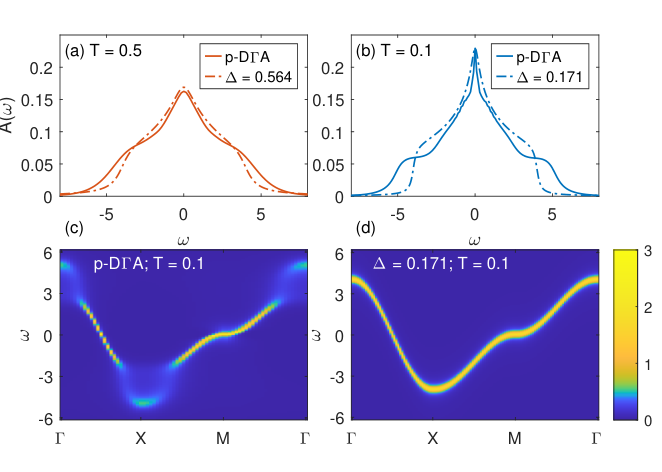
III Results

The focus of our calculations is on the vertex corrections to the Drude peak that are generated by -ton contributions. As already discussed, the simplest such contribution is the RPA ladder in the -channel shown in Fig. 2. In the following we will show results for the real part of the optical conductivity calculated directly on the real axis using Eq. (7) with a simplified two-particle vertex: either the RPA ladder of Eq. (9) or the Ornstein-Zernike form (11). The Green’s function is of the form Eq. (13) with a Fermi-liquid-like temperature dependence of the scattering rate , however with a constant offset. Specifically we use , which we obtained from a fit to p-DA see Appendix B.2 22 2 The value of the interaction in p-DA is , whereas here we use different values of . The reason is that the RPA series is a good approximation only for much smaller interaction values, and it grossly overestimates the AFM fluctuations. To represent in our approximate approach the intermediate coupling regime of , where -tons were observed, we hence need to use an effective value of in the RPA ladder, as it is done e.g. in the TPSC approach Vilk et al. 1994.. This featureless form of the Green’s function corresponds to the metallic phase of the Hubbard model 33 3 The fit we use will no longer be valid for the low temperature regime, , where we expect the pseudogap behavior in the Hubbard model Schäfer et al. 2015; Schäfer et al. 2021 . and gives per construction a Drude peak in the bubble part of the optical conductivity. Additional features in the bubble part, coming from frequency dependence of the self-energy (see e.g. Ref. Berthod et al. 2013), are neglected since we focus on the effect of vertex corrections on the two-particle level exclusively. In Appendix F we show that our conclusions are not changed if we assume a frequency dependent self-energy.
In the final subsection we also qualitatively compare the vertex corrections originating from the RPA ladder with constant self-energy with those from the -channel of the fully-fledged p-DA calculation.
III.1 Vertex corrections originating from RPA ladders in the transversal particle-hole channel


In Fig. 5 we show the effect of the RPA-ladder vertex corrections on the Drude peak for two different temperatures. The bubble contribution to the optical conductivity is a Drude peak per construction, since we used a simplified Green’s function with a constant imaginary part of the self-energy, depending only on temperature: . Our first observation is that including the vertex corrections does not change the overall shape of the peak and the full optical conductivity can still be fitted by a (Lorentzian) Drude peak. Both for the bubble as well as for the full vertex-corrected conductivity the Drude peak becomes sharper with decreasing temperature, as to be expected for a metal. Surprisingly however, it depends on the temperature, whether the vertex corrections broaden the Drude peak (, upper panel of Fig. 5) or sharpen it (, lower panel of Fig. 5). The vertex corrections are relatively small and their magnitude depends on the value of the effective interaction used in the RPA ladder (for the results presented in Fig. 5, ). We observe however similar behavior for other values of .
In Fig. 6 we analyze the temperature dependence in more detail. In the left column we show the full optical conductivity with RPA ladder vertex corrections for different temperatures and two values of the effective interaction and . These values of the effective interaction were chosen such that we are close to the divergence of the RPA-ladder, which indicates the AFM phase transition. This happens with our choice of for at and for at . The optical conductivity has the form of a Drude peak for all temperatures that we studied and the peak is broadened with increasing temperature. The latter is mainly due to the monotonic temperature dependence of the bubble contribution , shown in the right column of Fig. 6. Indeed that is exactly as to be expected for a Fermi-liquid-like metal. The RPA ladder vertex corrections (plotted in the middle column of Fig. 6) show however a strongly non-monotonic behavior. They broaden the Drude peak in the intermediate temperature regime (e.g., yellowish colors in Fig. 6 bottom), but lead to its sharpening for high temperatures (reddish colors in Fig. 6) and in particular for low temperatures (bluish colors). The latter is achieved by a vertex correction that is positive at the lowest frequencies and negative around (Fig. 6 top) respectively (Fig. 6 bottom).
For larger frequencies around the vertex corrections are always positive, independent of temperature. Together with the broadening and sharpening, this implies that in this region there are corrections to the Lorentzian-shape of the Drude peak. However, in this frequency region there will also be further contributions to the optical conductivity such as interband transitions (in multi-band systems), transitions to Hubbard bands, and our assumption of a constant self-energy is no longer justified since the Fermi liquid also implies a term , i.e., an increase of the one-particle scattering rate with frequency Berthod et al. 2013. Anyhow, except for this feature which is difficult to entangle from other effects and to observe in experiment, the RPA-ladder vertex corrections do not alter the Lorentzian form of the Drude peak, which is an important result by itself, besides of the non-monotonous temperature dependence of the broadening or sharpening.


This broadening and sharpening of the Drude peak is better illustrated in Fig. 7 (top panel) where we plot the difference between the full width of the peak and the width of the Drude peak from the bubble contribution as a function of temperature. Note that the Drude width of the numerically calculated bubble contribution agrees – as it should for a Fermi-liquid-like metal – with the one-particle scattering rate taken as input for the self-energy, i.e., 44 4 This relation holds for higher temperatures only approximately. . We clearly see three temperature regimes: (i) For the vertex corrections slightly sharpen the Drude peak (decrease its width, ) and the optical conductivity at is slightly increased (lower panel of Fig. 7) by the vertex corrections. This is also in agreement with an exact diagonalization study of vertex corrections beyond DMFT in Ref. Vučičević et al. 2019; Vranić et al. 2020 which was restricted to the high temperature regime. (ii) In an intermediate temperature regime, whose limits depend on the interaction value , the Drude peak is broadened by vertex corrections and the value (DC conductivity) is decreased. (iii) For the lowest temperatures we could reach, the vertex corrections sharpen the Drude peak and DC conductivity is increased. All effects become stronger and the intermediate temperature regime (ii) is enhanced when increasing the effective interaction , which enhances the AFM fluctuations.
In order to assess how important the temperature dependence of the scattering rate is for the temperature dependence of the vertex corrections, we perform a temperature scan with a fixed for all Green’s function lines [including the ones in the RPA ladder in Eq. (9)]. That is the temperature dependence enters solely via the Fermi and Bose distribution functions both in the bubble Eq. (5) and in the vertex part Eq. (7) 55 5 For clarity: the temperature enters in the RPA-ladder expression for the vertex, Eq. (9), through the Fermi distribution function present in .. In Fig. 8 we show the resulting RPA-ladder optical conductivity and its bubble and vertex parts for different temperatures at fixed . The non-monotonic behavior of the vertex corrections,, including all three temperature regimes (i)-(iii), is still present as a function of temperature. We thus see that while the temperature dependence of is quantitatively important, it is not needed for the correct qualitative behavior.
In Fig. 9 we present the value of the -ton RPA vertex contribution to the DC conductivity for different (inverse) temperatures and scattering rates treated as independent parameters. The green dashed line corresponds to the fit obtained from p-DA data as used in Figs. 5-7. The black line denotes the sign change of , which corresponds to the boundary between broadening (negative values, blue) and sharpening (positive values, red) of the Drude peak. Note that, as in Fig. 7, negative corresponds to an increase of the two-particle scattering rate , whereas positive , to a decrease of due to vertex corrections.
As is already clear from Fig. 8, keeping a constant scattering rate and increasing temperature, we go from sharpening to broadening and again to sharpening at high temperature, crossing the black line twice. In Fig. 9 this corresponds to moving along the green dashed line where we also cross the black line twice, which is due to the specific (quadratic with an offset) temperature dependence of , obtained from the p-DA fit. For large values of we do not see any sign changes in any more. We also cannot achieve the double sign change by changing at constant temperature. For the RPA vertex, the temperature dependence of the vertex corrections to the two-particle scattering rate (broadening and sharpening) is thus closely related to the temperature dependence of the one-particle scattering rate .
The conclusion from Fig. 9 is that low temperatures and a large one-particle scattering lead to a narrowing of the Drude peak [positive (red) ]. That we have two crossovers from narrowing to broadening and back again originates from the specific temperature-dependence of .
In this work we focus on two-particle vertex corrections to a featureless bubble contribution . Including consistently vertex corrections on both one- and two-particle level is a formidable task and was already done within the numerically cumbersome parquet approach in Ref. Kauch et al. 2020. However, in order to at least briefly assess how our results would change if we also introduced the same vertex corrections in the calculation of one-particle scattering rate, we computed the optical conductivity including these vertex corrections also in the one-particle Green’s functions in Eq. (3). Note that self-energy (scattering) rate and vertex corrections are related by the Schwinger-Dyson equation, see Appendix E. The results are presented in Appendix F and they show that the overall behavior of the vertex corrections is not changed – we also see temperature dependent broadening and sharpening of a slightly modified Drude peak (see Figs. 24- 25).
III.2 Effective vertex given by the Ornstein-Zernike form
In order to assess if the RPA-ladder effects are still present if we use a different form of the vertex that resembles the magnetic susceptibility, we have calculated vertex corrections with an Ornstein-Zernike (OZ) vertex of Eq. (11). The temperature dependence of the free parameters, , and the correlation length was obtained by fitting the RPA vertex with the OZ form Eq. (11). The details of the fits including the temperature dependencies of OZ parameters are presented in Appendix B.3.
In Fig. 10 we show the optical conductivity obtained from the OZ vertex Eq. (11). Here, we use for the two particle and two hole Green’s functions connecting the OZ vertex in the channel to the incoming and outgoing light exactly the same simple frequency-independent scattering rate (self-energy) as in the RPA (where this Green’s function was additionally employed for calculating the vertex itself). That is, when changing temperature, we change the Green’s function lines in the bare bubble and the four Green’s function outer lines in the vertex diagram (cf. Fig. 1), but the vertex itself is not diagrammatically built from Green’s function lines. Its temperature dependence enters only via the OZ parameters. The most important parameter is the AFM correlation length which is strongly temperature dependent as the inset of Fig. 10 shows; the two other parameters can be found in Appendix B.3. Knowing this dependence (here from fitting to the RPA vertex), we can translate temperature to AFM correlation length. This way we can look at the sign and shape of vertex corrections to the optical conductivity as a function of in Fig. 10.
Even with a simplified OZ form of the vertex, we see the same effect (now driven by changing ). The Drude peak is sharpened for large correlation lengths (corresponding to low temperatures) and broadened for smaller ’s. We did not reach the high temperature regime since we restricted the plot to (i.e. ), so the other sharpening regime at high is not present in the plot.
The form of the effective OZ vertex allows us to use the OZ parameters as additional knobs that we can turn independently of or , for helping us understand the origin of the non-monotonic temperature-dependence of the vertex corrections. In Fig. 11 we do exactly this: in each panel we change one of the three relevant parameters (correlation length , temperature , and one-particle broadening ) and keep the others as well as and of the OZ vertex fixed. The parameters were chosen so that we move away from the point with and , denoted with a black square in Fig. 9. Note that, since we use a fixed OZ-vertex here, changing or does not correspond to moving along lines in Fig. 9, where the vertex was from RPA.
In Fig. 11 (left panel) we see that changing , which is the key parameter for the temperature-dependent enhancement of the antiferromagnetic correlations at , changes the vertex corrections from a dampening in the intermediate temperature range (ii) to the sharpening in the low temperature range (iii). A comparison with Fig. 10 (middle panel) however also shows already that other factors must be at work as well.
The two other parameters, i.e., in Fig. 11 (middle panel) and (right panel), only enter in the four Green’s function lines connecting the (now fixed) OZ vertex with the incoming and outgoing light. These parameters change the frequency range () over which vertex contributions are included. The temperature yields also an important contribution to the broadening in the intermediate temperature regime (ii) and a sharpening at low temperatures (iii); whereas is less relevant at low temperature where it hardly changes, but important for the sharpening in the high temperature regime (i). Please also note the isosbestic point Greger et al. 2013 around . In terms of the frequency integrals Eq. (8) around the branch cuts, always yields a positive vertex correction and a negative one (except for very high temperature, when it can become positive), but depending on , , and , the total balance is changing sign.
An analogous parameter scan as done in Fig. 11 for parameters close the low temperature regime in Fig. 9 (black square), was done for a high temperature in the vicinity of two values of (points denoted by black circle and magenta triangle in Fig. 9). A detailed analysis is presented in Appendix C. The overall conclusion is that in case of the OZ vertex used in the high temperature regime, the vertex corrections lead to sharpening (increased value of ) only at large values of or when setting the correlation length very small (see Fig. 17). This was not the case for the RPA vertex. We note, that for high temperatures the correlation length description of the system provided by the OZ vertex is no longer valid and the RPA and OZ vertices differ more.
III.3 Relation to the parquet DA results
The -ton contributions to optical conductivity, as described in Ref. Kauch et al. 2020, are not directly identifiable with ladder diagrams only. In fact, without insertions from other channels, the -ladder diagrams would eventually diverge at when lowering the temperature in the systems with strong AFM/CDW fluctuations. These diagrams though, even if dampened by other contributions, provide the dominant part of the -channel. It is however not obvious if the simplest approach, where the ladder is built only with a constant effective as the interaction vertex, can describe the same physics as the full p-DA calculation.
In Fig. 12 we show a qualitative comparison between the p-DA vertex corrections (at ) and the RPA-ladder ones (at two values of the effective interaction and ) in a range of temperatures. Even though the Green’s functions were simplified in the RPA ladders, the qualitative behavior with temperature in both approaches is similar: a sharpening at the lowest temperature and broadening in the higher temperature regime. We show here only the low frequency range, since for higher frequencies there are effects coming from the (precursors of the) Hubbard bands that are absent in the calculation with the constant self-energy. Another important difference between the p-DA and RPA results is the analytic continuation: it had to be done numerically in p-DA, whereas in RPA we derived and used expressions in real frequencies.
IV Conclusion
Motivated by the work on -ton contributions to the optical conductivity Kauch et al. 2020 and the importance of the AFM and CDW fluctuations for vertex corrections in strongly correlated electron systems, we have studied in this paper their influence on the Drude peak in a simplified semi-analytical calculation. To this end, we have employed the RPA ladder for studying one vertex correction that is especially effective and indeed the diagrammatic archetype for strong AFM or CDW fluctuations. In order to couple this ladder which becomes large for a wave vector to light with , we need to built the ladder in the transversal particle-hole channel. Here, two particle-hole pairs are created by the incoming and outgoing light, respectively. For one pair, particle and hole carry the momentum and for the other . This allows the coupling to AFM and CDW fluctuations at . While antiferromagnetic fluctuations are quintessential for the Hubbard model, in other parameter regimes and for other lattices e.g. superconducting or ferrmognetic fluctuations may dominate and with this other channels may become important.
In the context of high-temperature superconductivity a classification of vertex corrections into Maki Maki 1968-Thompson Thompson 1970 and Aslamazov-Larkin (AL) Aslamazov and Larkin 1968 type is sometimes employed, also in the context of the optical, Hall and Raman conductivity Kontani et al. 1999; Kontani 2008; Kampf and Brenig 1992; Bergeron et al. 2011; Chubukov et al. 2014. The -ton or transversal particle-hole channel is a different classification: diagrams of both, the MT and AL class 66 6 The second order in diagram of the RPA ladder is of AL, the others are of MT type; there is no first order diagram., contribute to the -tons in the ladder.
By using a simplified vertex we have made it possible to calculate the optical conductivity with vertex corrections on the real frequency axis 77 7 For the functional renormalization group Metzner et al. 2012, which is related to the parquet through its multiloop extensions Kugler and von Delft 2018; Hille et al. 2020 a simplified quasiparticle description directly on the real axis has been recently proposed Rohe and Honerkamp 2020. For a p-DA additionally a local vertex for real frequencies is needed, which one might obtain, e.g., through matrix product states Bauernfeind et al. 2017 and we derived the necessary analytical expressions for this purpose. These expressions are general and can be used for arbitrary Green’s function known on the real axis and a vertex that has the same frequency structure in the complex plane as a physical susceptibility. In this way we avoid the uncertainty that is sometimes present in the analytic continuation of numerical data obtained on the Matsubara axis and have sufficient momentum resolution. This allows us to study changes reliably also for small vertex corrections and to understand whether the simplest RPA-ladder diagrams in the channel are sufficient to explain the numerical results of Ref. Kauch et al. 2020.
As for the validity of our calculations, we can only expect an RPA-based approach to be at least qualitatively reliable at weak coupling in the metallic phase. By construction, our approach is further limited to the parameter regimes, where the contributions are indeed dominant, i.e. when AFM or CDW fluctuations are prevalent 88 8 Please note that within the RPA-approach using an effective interaction is necessary, and hence we cannot reliably treat different channels on an equal footing.. As was shown in Ref. Kauch et al. 2020, for the considered parameter range the channel is indeed the dominant vertex corrections to the optical conductivity; the second largest is from the channel; the channel is large at but its overall contribiution to the optical conductivity with is weak.
We first of all find that the RPA-ladder -ton contributions do not alter the overall Lorentzian shape of the Drude peak in the low frequency regime–at least in the weak coupling domain of RPA. The width of the Drude peak for a given temperature is however modified by the ladder -tons: the peak is sharpened at low and high temperatures, but broadened for intermediate temperatures. That there are two such crossovers eventually originates from the temperature-dependence of the single-particle scattering rate which has a larger curvature than the crossover from broadening at high and low to sharpening at low and high in Fig. 9. The sharpening at high temperatures through vertex corrections has been observed also in Ref. Vučičević et al. 2019. For slightly higher frequencies, where the Drude peak has only a Lorentzian tail we see some additional feature coming from vertex corrections, that are positive at all temperatures. This frequency range though is not very well represented by the approximate constant self-energy that we used and a closer look in this regime goes beyond our simplified study.
For a half-empirical calculation of -ton vertex corrections one could use the magnetic susceptibility, as was suggested already in the supplemental material to Ref. Kauch et al. 2020. Here we have shown in a model calculation that one can replace the RPA ladder by a universal Ornstein-Zernike form. The aforementioned sharpening-broadening-sharpening upon lowering temperature originates from both, the enhancement of the vertex around due to an increase of the correlation length and the reduction of its relevant frequency window. The latter is because the two -ton particle-hole excitations coupled to the incoming and outgoing light must be closer and closer to the Fermi energy with decreasing temperature in the low frequency range of the optical spectrum.
The final question that we have tried to answer in this work is whether the simplest ladder diagrams in the -channel are enough to at least qualitatively address the -tons in the 2D Hubbard model. For the low frequency part of the optical conductivity, the answer seems to be positive, since the main effect, a non-monotonic temperature dependence resulting in broadening or sharpening of the Drude peak by the -ton contributions is analogous in p-DA and in the RPA-ladder approach.
Note added: During the completion of our work, we became aware of an independent calculation of -ton contributions to optical conductivity using RPA Simard et al. 2021 with a different physics focus, mainly on the 1D Hubbard model, and some differences in the implementation.
Acknowledgments. We would like to thank K. Astleithner, J. Kuneš, and P. Pudleiner for many stimulating discussions. This work was supported by the Austrian Science Fund (FWF) through projects P 30819 and P 30997, and the Doctoral School W 1243 “Building Solids for Function”. Calculations have been done on the Vienna Scientific Cluster (VSC).

Appendix A Derivation of the real frequency optical conductivity with vertex corrections
In this Appendix we provide an explicit derivation of the real frequency expressions used for the numerical calculation of the current-current correlation function —the full one as well as its constituents, the bare bubble and vertex correction. The real part of the optical conductivity is then given by evaluating the expression . To make the notation clearer we use in the following a different notation for Matsubara frequencies: i.e., we denote the imaginary fermionic frequencies by and the bosonic by (with ). The real frequencies are or . We also keep the general bosonic momentum dependence of the current-current correlation function and skip the subscript in the following.
A.1 Bubble contribution
To make the notation and assumptions clear we repeat a derivation of Eq. (5) for the bare bubble contribution on the real frequency axis. Without vertex corrections the expression of interest is in Matsubara frequencies
| (15) |
where the sign originates from the fermionic loop rule and the factor two is due to the spin. The Matsubara sums in Eq. (15) can be translated into a real frequency integral by using the fact that the fermionic Matsubara frequencies are located at the poles of the Fermi-Dirac distribution and that is analytical everywhere except for the real axis (where it has a branch cut). For () the Green’s function is the analytic continuation of the retarded (advanced) Green’s function (). This leads to
| (16) |
where the contours encircle all the singularities of of . By Cauchy’s theorem the contours can be deformed arbitrarily, unless they encounter a region of ambiguous analyticity. For the above expression these regions are located at and at . After stretching the contours in such a ways that they cover the whole complex plane, except for stripes of infinitesimal height at and at , it can be shown that the stripes give the only nonzero contribution. The arcs of (infinite radius) that close the contour do not give a contribution because the integrand is decaying faster than . One can therefore rewrite Eq. (16) as
| (17) |
Here, we used that and . We also assumed that , which may be referred to as the dynamic limit. Using that the analytical continuation of the Green’s function from above/below the branch cut gives (which are in equilibrium related to one another by complex conjugation) and denoting the spectral function as we get
| (18) |
After transforming all Matsubara sums into integrals over real frequencies the remaining analytical continuation amounts to a simple substitution .
A.2 Vertex Corrections
In this Section we derive Eq. (8), starting again from the expression in Matsubara frequencies, but now for the vertex corrections:
| (20) |
The analytic continuation of Eq. (20) follows the same procedure as for the bubble contribution. We again assume (dynamic limit). The order in which the Matsubara sums are evaluated does not matter. Here we present the evaluation of the -sum first [ in 20]. The complex structure of the single frequency vertex must be the same as that of a physical magnetic susceptibility, i.e., is analytical in the whole complex plane except for where it has a branch cut 99 9 as explained in Eq. (II.2). The RPA-Bubble (9) as well as the Ornstein-Zernike-susceptibility (10) fulfill this assumption. Since branch-cuts appear in both the Green’s function and the one-frequency vertex , when the imaginary part of the frequency argument vanishes, there are three branch cuts when we analytically continue the argument of the Matsubara sum into the whole complex plane, cf. Fig. 13:
| (21) |
The first one, (i) in Eq. (21), originates from the vertex in Eq. (20), which has a branch cut between retarded and advanced vertex at or . Branch cuts Eq. (21) (ii) and (iii) are from the two Green’s functions and , respectively. Special care has to be taken additionally since the first branch-cut in Eq. (21) is on top of a pole. Thus the point has to be explicitly excluded from the second Matsubara sum and treated separately:
| (22) |
Here, we introduced . The contours enclose all Matsubara frequencies of the sum except for and are visualized in Fig. 13 as well.
Again the arches (of infinite radius) do not contribute to the integral because the integrand decays faster than . The only remaining contributions come from the three stripes in Fig. 13 (leftward and rightward integral with infinitely small separation in-between), mathematically given by
| (23) |
For the second term () we used . For the singularity of the Bose-Einstein function on can use a variation of the Plemelj-Sokhotskii theorem Sokhotskii 1873 that given a well behaved (holomorphic) function reads
| (24) |
The -term can be split up into two parts, where the contributions due to the delta-distribution cancels exactly the term 1010 10 We present here the solution for . While this is true for the systems considered here (RPA, Ornstein-Zernike) it is not correct for some special cases (e.g. non-ergodic systems Wilcox 1968; Kwok and Schultz 1969; Suzuki 1971). The general procedure does, however, not change. The only difference being that the term does no longer cancel. Instead one gets the as an additional contribution, but with instead of .:
| (25) |
In the last line of Eq. (25) we used that and that the singularity of gets regularized by . The Cauchy-principle value can therefore be replaced by a normal integral. Inserting Eq. (23) into Eq. (20) and reordering in such a way that all terms containing are together leads to
| (26) |
| (27) |
In Eq. (27) we further need to transform the Matusbara sums over the first index in Eq. (20) into contours integrals enclosing all poles of the Fermi-Dirac distribution function . All terms have branch-cuts at two additional lines regarding the analytically continued first summation index , namely at
| (28) |
Altogether we hence need to account for five branch cuts, when we analytically continue the Matsubara frequency sums and to real frequency integrations.
Inserting Eq. (27) into Eq. (23) and performing the last analytical continuation of the external frequency by substituting gives
| (29) |
with
| (30) |
and
| (31a) |
In Eq. (33b) we combined plus into the sum so that each individual term fulfills the symmetry for .
Appendix B Computational Details
B.1 and grid sizes
For all calculations presented we used the -grid of at least points. The numeric frequency integration was done using trapezoidal rule with at least points within the frequency range of .
B.2 Drude fit to pDA bubble
In order to obtain the temperature dependent scattering rate , we used a -fit of the Drude form to the analytically continued bubble contribution of the p-DA optical conductivity obtained in Ref. Kauch et al. 2020 for different temperatures and the bare interaction value of . Both the Drude fit, as well as the original p-DA bubble contribution are shown in the left panel of Fig. 14 for different temperatures. The extracted temperature dependence together with a fit is shown in the right panel of Fig. 14.
B.3 Fit of the Ornstein-Zernike vertex to the RPA ladder vertex
We extract the parameters of the Ornstein-Zernike vertex of Eq. (11): , , through a -fit to the real part of the RPA-ladder vertex Eq. (9). All three parameters are, however, not extracted simultaneously. First and are obtained by fitting to the value at . Then, keeping and constant, is obtained by a -fit to the dependence. A comparison of the fitted OZ vertex to the RPA vertex is shown in Fig.15.
Fig. 16 in turn displays the extracted parameters of the Ornstein-Zernike vertex as a function of temperature (symbols). The solid lines represent a fitted temperature behavior of the form , except for fitting at , where an exponential fit of the form had to be employed to account for the strong increase at low temperatures, see purple line in Fig. 17 (left). The respective fit parameters are given in Table 1.
| 1.7 | 1.8 | 1.9 | 1.7 | 1.8 | 1.9 | 1.7 | 1.8 | 1.9 | |||
|---|---|---|---|---|---|---|---|---|---|---|---|
| 0.63 | 0.53 | 0.41 | 10.6 | 11.7 | 13.0 | -1.15 | -1.08 | -1.03 | |||
| -0.19 | 0.26 | 0.30 | 0.36 | 0.11 | 1e-3 | 0.83 | 1.33 | 0.51 | |||
| 0.53 | 0.46 | 0.38 | 10.9 | 10.7 | 10.6 | -1.39 | -1.37 | -1.29 | |||
Appendix C Ornstein-Zernike vertex corrections to the optical conductivity for high temperature
In the high temperature regime we see a transition between broadening of the Drude peak and its sharpening when the temperature is increased in case we use the RPA vertex. This is illustrated in Fig. 9, where for high temperatures or large the vertex corrections are positive. We choose now two points on the green line, with and (black circle in Fig. 9) and with and (magenta triangle in Fig. 9) and perform an OZ-fit to the RPA vertex for each of them. With the obtained OZ parameters, we calculate the vertex corrections with the OZ vertex instead of the RPA vertex. The results for the two different ways of calculating , i.e. directly from the RPA vertex or alternatively from OZ vertex with parameters fitted on RPA, are shown in the leftmost plot in Fig. 17. Solid lines denote the RPA vertex corrections that change sign when we move from the black circle (black in Fig. 17) to the magenta triangle (magenta). Dashed lines denote the OZ results for these points. We do not see a sign change for the OZ vertex, although its parameters were fitted to the RPA vertex. We neither see a sharpening of the Drude peak at high temperature with thus fitted OZ vertex.
In order to check if it is at all possible to obtain positive vertex corrections with the OZ vertex, we choose the black circle of Fig. 9 as a starting point and change the temperature, correlation length and treating them as independent parameters, as was done in Fig. 11 for a lower temperature. We show in Fig. 17 only the value of as a function , , and , with other parameters kept fixed (left middle, right middle, and rightmost plot, respectively). With lowering the temperature we enter the sharpening regime with the OZ vertex as well, even if we keep the correlation length fixed. Staying at higher temperature () however, we get positive values of only at or with a very small correlation length . In the small correlation length or large scattering rate regime, the vertex corrections become positive at high temperature even with the OZ form of the vertex.
Let us note, however, that at high temperature the correlation length description of the system is not any more adequate, which also explains the differences between OZ and RPA results. The correlation between next neighbors still changes with the correlation length if it is somewhat below 1. As a matter of course in this regime the description by means of a correlation length is not accurate any more, as also the quite substantial deviation from the Ornstein-Zernike form for in Fig. 15 (left) shows.
Appendix D RPA ladders in and channels
Motivated by the results of Ref. Kauch et al. 2020, we state in Sec. IV, that the dominant contribution to the vertex correction to optical conductivity comes from an RPA-type ladder in the channel. Here we discuss all possible contributions from ladder-type diagrams in the and channels and explain why RPA-type ladders other than in the magnetic channel are not important.
Assuming SU(2) spin-symmetry, the vertex entering Eq. 4 is the full two-particle vertex in the density spin channel Bergeron et al. 2011, which (in the notation of Ref. Rohringer et al. 2018) is defined as
| (34) |
where we used a shortened notation of for and for . The remaining independent spin combination is , which we denote by . For completeness we also introduce the magnetic spin channel
| (35) |
Using the parquet decomposition Rohringer et al. 2018 allows for unambiguous classification in terms of two-particle reducibility, see Fig. 18,
| (36) |
with denoting the set of fully irreducible diagrams (diagrams that are not reducible in , nor , nor channels).
All RPA-like ladders are by construction reducible in one of the three channels. Each channel contains three ladders, one for each of the three spin combinations (, , ). For the and channels these are given by:
| (37a) | ||||
| (37b) | ||||
| (37c) | ||||
| (37d) | ||||
| (37e) | ||||
| (37f) | ||||
with . The first two diagrams of those RPA-like ladders are also displayed in Fig.19 (in the channel) and Fig.20 (in the channel). Note, that they have a reduced frequency-momentum dependence and depend only either on ( channel) or on ( channel).
If we restrict ourselves only to such RPA-like ladders and assume the pp-channel to be small as observed in Ref. Kauch et al. 2020 the vertex in Eq. (34) can be written as,
| (38) |
Using the so-called crossing symmetry that connects the and channels (see e.g. Ref. Rohringer et al. 2018),
| (39) |
one can rewrite Eq. 38 in order to express everything in the -channel only
| (40) |
where we omitted in ’s the first two (fermionic) frequency-momentum arguments, because in the RPA-ladder approximation in the -channel they depend only on the third, bosonic, argument (see Eqs. (37)). Note, that such constructed vertex obeys the crossing-symmetry, as opposed to a single RPA ladder in the channel.

The first two contributions to in Eq. (40) do not give any vertex correction to the optical () conductivity for a one-band model. This is because is anti-symmetric in k, while is symmetric and therefore any vertex that depends only on but not on will give zero when inserted in Eq. (4).
For the remaining part () in Eq. (40) we can assume, that the magnetic channel will dominate because and and , . In Fig. 21 we show a comparison of vertex contributions from the density and magnetic channels. The density channel contribution is indeed much smaller, even though we take the same value of the effective in this calculation. In fact, taking a different value of the effective interaction in the density channel (less screened than in the magnetic channel) would make the contribution even smaller. Considering only the dominant magnetic channel, which corresponds to the diagram as drawn in Fig. 2, Sec. II.3, allows us also avoiding the problem of choosing appropriate effective Bergeron et al. 2011, leaving only one effective (magnetic) -value that we treat as a free parameter in our model calculation.
Appendix E Schwinger-Dyson equation in real frequencies for a vertex depending on one frequency
The Schwinger-Dyson equation connects the two-particle vertex to the one-particle self-energy and reads for the Hubbard-Hamiltonian Rohringer et al. 2018:
| (41) |
The first term in Eq. (41) is the Hartree-term, which is not important for the following discussion and will hence be omitted for simplicity.
To be specific we will proceed with the RPA-like ladder approximation of the vertex, as presented in Appendix C, but the final equation can be used for any vertex that depends on only one frequency ( in Eq. (44)). In RPA we will omit the contribution from the -channel and take only the and ladders in the Schwinger-Dyson equation. Note that while the contribution of ladder to the optical conductivity can be neglected, as discussed in Appendix D, this is not the case for the contribution to the self-energy (as neither the restriction to nor the antisymmetry of the enters). Including both, and ladders, in yields
| (42) |
where we used the crossing symmetry Rohringer et al. 2018 in the second line and in the notation of the third line we omitted the first two fermionic variables, since the -ladder depends only on the last, bosonic variable, as shown in Eq. (37).

In this approximation Eq. (41) can be rewritten as:
| (43) |
From now on we will explicitly distinguish between the bare interaction value, which we now denote with , and the effective (screened) that we take as the RPA vertex.
Eq. (43) can be further simplified by using again and employing a variable change and for the third term.
| (44) |
The real frequency version of Eq. (44) can be obtained following along the same lines as in Section A. Branchcuts are at and . Rewriting the Matsubara sum in terms of integrals yields,
| (45) |
The above expression can be used for calculating the self-energy for a general , provided the reduced frequency dependence.

In Fig. 22 we show the real and imaginary part of the self-energy as a function of frequency for two points in the Brillouin zone, for several temperatures, as obtained from Eq. (45) with the RPA vertex as in Eq. (44). The input self-energy to calculate the RPA vertex as well as the one-particle Green’s functions was the constant but temperature dependent self-energy we used in the main text (see Sec. II.6), with . We performed here only a one-shot calculation. Further improvement could be achieved (albeit at a significant numerical cost) by using e.g. the two-particle self-consistent approach as in Ref. Bergeron et al. 2011. We used here the bare interaction value of , which corresponds to the value from the parquet DA calculation of Ref. Kauch et al. 2020 (as the bare enters the Schwinger-Dyson equation) and the effective interaction in the RPA ladders (as beyond RPA ladder contributions reduce the magnetic fluctuations).
The self-energy in Fig. 22 shows the typical Fermi liquid behavior with a linear -dependence for the real part of the self-energy and a quadratic behavior for the imaginary part 1111 11 Particular strong scattering at the van Hove singularity will be cut-off by the finite scattering rate of the the starting self-energy. On top of this quadratic -dependence, there is a finite scattering rate that is suppressed upon decreasing temperature. This low energy scattering is more pronounced for the antinodal point , as one can also see in momentum dependence of the self-energy at the Fermi level () shown in Fig. 23. Despite this momentum differentiation there is no sign for the formation of a pseudogap, which would be signaled by a pole in the real part of the self-energy. Please note that, while showing a reasonable Fermi liquid frequency dependence, this RPA recalculated self-energy cannot be considered (in the frequency range relevant for the Drude peak) to be superior to the constant fitted to the more precise numerical parquet data. Indeed due to anti-ferromagnetic fluctuations the low frequency scattering rate will not vanish but after a plateau increase again at low temperatures Rohringer and Toschi 2016. In the next Section, we will see that the difference between the fitted constant self-energy and the RPA recalculated self-energy in any case does not alter our conclusions.
Appendix F The effect of RPA-ladder vertex corrections to self-energy on the optical conductivity
Throughout the main paper we used a model, featureless, self-energy as described in Sec. II.6. This approach does not capture the interplay between vertex corrections to one- and two-particle quantities. It is however not feasible to apply a fully one- and two-particle consistent approach, as e.g. the parquet approach of Ref. Kauch et al. 2020 does, and to keep the same momentum resolution or do calculations on the real frequency axis. In the following we only try to assess if and how including the frequency dependence and self-consistency effects for the self-energy alters our conclusions of the main text. To this aim we use the self-energy with a vertex correction from Eq. (45) in the calculation of the optical conductivity. We make only a one-shot correction, which means the self-energy from Eq. (45) is used only in the bubble contribution and in the outer lines in Eq. (3), but the vertex entering Eq. (7) is calculated with Green’s functions for which we use the constant scattering rate as described in the main text. This way the vertex used in Eq. (45) and Eq. (7) is the same.
The results are shown in Fig. 24, which is constructed analogously to Fig. 6. We also see the three temperature regimes: (i) a sharpening for high temperatures; (ii) broadening in the intermediate regime; (iii) and again sharpening in the low temperature regime. Quantitatively now both the bubble contribution as well as the vertex corrections are larger at at low temperatures, which is caused by the reduced scattering rate around (compared to the constant we took in the model Green’s function in the main text) as can be seen in the imaginary part of the self-energy in Fig. 22. The qualitative behavior in the lowest frequency regime is however unchanged. In particular the lowest frequency regime of both the full optical conductivity and the bubble contribution can still be well fitted with a Drude peak. For intermediate frequencies, , we see a different behavior already in the bubble contribution. Also the vertex corrections do not become negative in this frequency regime as it was visible in Fig. 6 for a frequency independent self-energy. These differences come from the strong frequency dependence of the self-energy for the intermediate frequency range (cf. Fig. 22).
In Fig. 25 we present, in analogy to Fig. 7, the difference between the width of the Drude peak fitted to full optical conductivity and fitted to only the bubble contribution . Also the vertex corrections to the DC conductivity are shown. We again see the sharpening–broadening–sharpening behavior with temperature. Overall the corrections to are larger as already seen in Fig. 24. The corrections to the width of the Drude peak on the other hand are smaller than the ones in the case of constant self-energy (cf. Fig. 7).
We could alternatively do a different calculation and also use the vertex corrected self-energy to obtain an updated RPA vertex and then calculate the vertex correction with Eq. (7). The outer and inner Green’s function lines in the calculation of optical conductivity from Eq. (3) would then be the same (where by ’inner lines’ are the Green’s functions used to calculate the RPA vertex). We have done so but this additional self-energy feedback to the vertex has only minor influence on the vertex corrections to optical conductivity and is hence not shown here.
References
- Drude (1900a) P. Drude, Zur elektronentheorie der metalle, Annalen der Physik 306, 566 (1900a).
- Drude (1900b) P. Drude, Zur elektronentheorie der metalle; ii. teil. galvanomagnetische und thermomagnetische effecte, Annalen der Physik 308, 369 (1900b).
- Sommerfeld (1928) A. Sommerfeld, Zur Elektronentheorie der Metalle auf Grund der Fermischen Statistik, Z. Physik 47, 1 (1928).
- Frenkel (1931) J. Frenkel, On the transformation of light into heat in solids. i, Phys. Rev. 37, 17 (1931).
- Wannier (1937) G. H. Wannier, The structure of electronic excitation levels in insulating crystals, Phys. Rev. 52, 191 (1937).
- Maebashi and Fukuyama (1997) H. Maebashi and H. Fukuyama, Electrical conductivity of interacting fermions. i. general formulation, Journal of the Physical Society of Japan 66, 3577 (1997).
- Peierls (1930) R. Peierls, Zur theorie der elektrischen und thermischen leitfähigkeit von metallen, Annalen der Physik 396, 121 (1930).
- Kontani (2008) H. Kontani, Anomalous transport phenomena in fermi liquids with strong magnetic fluctuations, Reports on Progress in Physics 71, 026501 (2008).
- Maslov and Chubukov (2017) D. L. Maslov and A. V. Chubukov, Optical response of correlated electron systems, Rep. Prog. Phys. 80, 026503 (2017).
- Keimer (2013) B. Keimer, Autumn School on Correlated Electrons.emergent phenomena in correlated matter (Forschungszentrum Jülich, 2013) Chap. Recent Advances in Experimental Research on High-Temperature Superconductivity.
- Aeppli (2004) G. Aeppli, The ubiquity of antiferromagnetism in strange solids, Journal of Magnetism and Magnetic Materials 272-276, 7 (2004).
- Kauch et al. (2020) A. Kauch, P. Pudleiner, K. Astleithner, P. Thunström, T. Ribic, and K. Held, Generic optical excitations of correlated systems: -tons, Phys. Rev. Lett. 124, 047401 (2020).
- Clarke (1993) D. G. Clarke, Particle-hole bound states in mott-hubbard insulators, Phys. Rev. B 48, 7520 (1993).
- Wróbel and Eder (2002) P. Wróbel and R. Eder, Excitons in mott insulators, Phys. Rev. B 66, 035111 (2002).
- Essler et al. (2001) F. H. L. Essler, F. Gebhard, and E. Jeckelmann, Excitons in one-dimensional mott insulators, Phys. Rev. B 64, 125119 (2001).
- Jeckelmann (2003) E. Jeckelmann, Optical excitations in a one-dimensional mott insulator, Phys. Rev. B 67, 075106 (2003).
- Kontani (2006) H. Kontani, Optical conductivity and hall coefficient in high-tc superconductors: Significant role of current vertex corrections, Journal of the Physical Society of Japan 75, 013703 (2006).
- Lin et al. (2009) N. Lin, E. Gull, and A. J. Millis, Optical conductivity from cluster dynamical mean-field theory: Formalism and application to high-temperature superconductors, Phys. Rev. B 80, 161105 (2009).
- Chubukov et al. (2014) A. V. Chubukov, D. L. Maslov, and V. I. Yudson, Optical conductivity of a two-dimensional metal at the onset of spin-density-wave order, Phys. Rev. B 89, 155126 (2014).
- Bergeron et al. (2011) D. Bergeron, V. Hankevych, B. Kyung, and A.-M. S. Tremblay, Optical and dc conductivity of the two-dimensional hubbard model in the pseudogap regime and across the antiferromagnetic quantum critical point including vertex corrections, Phys. Rev. B 84, 085128 (2011).
- Vučičević et al. (2019) J. Vučičević, J. Kokalj, R. Žitko, N. Wentzell, D. Tanasković, and J. Mravlje, Conductivity in the square lattice hubbard model at high temperatures: Importance of vertex corrections, Phys. Rev. Lett. 123, 036601 (2019).
- Pudleiner et al. (2019) P. Pudleiner, P. Thunström, A. Valli, A. Kauch, G. Li, and K. Held, Parquet approximation for molecules: Spectrum and optical conductivity of the pariser-parr-pople model, Phys. Rev. B 99, 125111 (2019).
- Astleithner et al. (2020) K. Astleithner, A. Kauch, T. Ribic, and K. Held, Parquet dual fermion approach for the falicov-kimball model, Phys. Rev. B 101, 165101 (2020).
- Bickers (2004) N. E. Bickers, Theoretical methods for strongly correlated electrons (Springer-Verlag New York Berlin Heidelbert, 2004) Chap. 6, pp. 237–296.
- Yang et al. (2009) S. X. Yang, H. Fotso, J. Liu, T. A. Maier, K. Tomko, E. F. D’Azevedo, R. T. Scalettar, T. Pruschke, and M. Jarrell, Parquet approximation for the hubbard cluster, Phys. Rev. E 80, 046706 (2009).
- Li et al. (2016) G. Li, N. Wentzell, P. Pudleiner, P. Thunström, and K. Held, Efficient implementation of the parquet equations: Role of the reducible vertex function and its kernel approximation, Phys. Rev. B 93, 165103 (2016).
- Li et al. (2017) G. Li, A. Kauch, P. Pudleiner, and K. Held, The victory project v1.0: an efficient parquet equations solver, Comput. Phys. Commun. , 146 (2017).
- Valli et al. (2015) A. Valli, T. Schäfer, P. Thunström, G. Rohringer, S. Andergassen, G. Sangiovanni, K. Held, and A. Toschi, Dynamical vertex approximation in its parquet implementation: Application to hubbard nanorings, Phys. Rev. B 91, 115115 (2015).
- Rohringer et al. (2018) G. Rohringer, H. Hafermann, A. Toschi, A. A. Katanin, A. E. Antipov, M. I. Katsnelson, A. I. Lichtenstein, A. N. Rubtsov, and K. Held, Diagrammatic routes to nonlocal correlations beyond dynamical mean field theory, Rev. Mod. Phys. 90, 025003 (2018).
- (30) The numerical bottleneck is in particle the memory consumption of a general vertex depending on three frequencies and three momenta, which might be mitigated in the future by an efficient sparse parameterization thereof Honerkamp 2018; Shinaoka et al. 2020; Li et al. 2020; Eckhardt et al. 2020; Krien et al. 2021.
- Altshuler and Aronov (1985) B. L. Altshuler and A. G. Aronov, Electron-Electron interaction in disordered conductors, edited by A. I. Efros and M. Pollak (Elsevier Science Publisher, 1985).
- Rammer (1998) J. Rammer, Quantum Transport Theory (CRC Press, 1998).
- Peierls (1933) R. Peierls, Zur Theorie des Diamagnetismus von Leitungselektronen, Z. Phys. 80, 763 (1933).
- Altland and Simons (2010) A. Altland and B. D. Simons, Condensed Matter Field Theory, 2nd ed. (Cambridge University Press, 2010).
- Jarrell and Gubernatis (1996) M. Jarrell and J. E. Gubernatis, Bayesian inference and the analytic continuation of imaginary-time quantum monte carlo data, Phys. Rep. 269, 133 (1996).
- Mishchenko et al. (2000) A. S. Mishchenko, N. V. Prokof’ev, A. Sakamoto, and B. V. Svistunov, Diagrammatic quantum monte carlo study of the fröhlich polaron, Phys. Rev. B 62, 6317 (2000).
- Otsuki et al. (2017) J. Otsuki, M. Ohzeki, H. Shinaoka, and K. Yoshimi, Sparse modeling approach to analytical continuation of imaginary-time quantum monte carlo data, Phys. Rev. E 95, 061302 (2017).
- Yoshimi et al. (2019) K. Yoshimi, J. Otsuki, Y. Motoyama, M. Ohzeki, and H. Shinaoka, Spm: Sparse modeling tool for analytic continuation of imaginary-time green’s function, Computer Physics Communications 244, 319 (2019).
- Tikhonov and Arsenin (1977) A. N. Tikhonov and V. I. Arsenin, Solutions to ill-posed problems (Winston ; distributed solely by Halsted Press Washington : New York, 1977) pp. xiii, 258 p. :.
- Kappl et al. (2020) P. Kappl, M. Wallerberger, J. Kaufmann, M. Pickem, and K. Held, Statistical error estimates in dynamical mean-field theory and extensions thereof, Phys. Rev. B 102, 085124 (2020).
- Galler et al. (2017) A. Galler, P. Thunström, P. Gunacker, J. M. Tomczak, and K. Held, Ab initio dynamical vertex approximation, Phys. Rev. B 95, 115107 (2017).
- Georges et al. (1996) A. Georges, G. Kotliar, W. Krauth, and M. J. Rozenberg, Dynamical mean-field theory of strongly correlated fermion systems and the limit of infinite dimensions, Rev. Mod. Phys. 68, 13 (1996).
- Kuneš (2011) J. Kuneš, Efficient treatment of two-particle vertices in dynamical mean-field theory, Phys. Rev. B 83, 085102 (2011).
- Löhneysen et al. (2007) H. v. Löhneysen, A. Rosch, M. Vojta, and P. Wölfle, Fermi-liquid instabilities at magnetic quantum phase transitions, Rev. Mod. Phys. 79, 1015 (2007).
- Hertz (1976) J. A. Hertz, Quantum critical phenomena, Phys. Rev. B 14, 1165 (1976).
- Millis (1993) A. J. Millis, Effect of a nonzero temperature on quantum critical points in itinerant fermion systems, Phys. Rev. B 48, 7183 (1993).
- Moriya and Kawabata (1973) T. Moriya and A. Kawabata, Effect of spin fluctuations on itinerant electron ferromagnetism, J. Phys. Soc. Jpn. 34, 639 (1973).
- Mahan (2000) G. D. Mahan, Many-Particle Physics (Kluwer Academic/Plenum Publishers, New York, 2000).
- Mahan (1966) G. D. Mahan, Mobility of polarons, Phys. Rev. 142, 366 (1966).
- Simard et al. (2021) O. Simard, S. Takayoshi, and P. Werner, Diagrammatic study of optical excitations in correlated systems, Phys. Rev. B 103, 104415 (2021).
- (51) The value of the interaction in p-DA is , whereas here we use different values of . The reason is that the RPA series is a good approximation only for much smaller interaction values, and it grossly overestimates the AFM fluctuations. To represent in our approximate approach the intermediate coupling regime of , where -tons were observed, we hence need to use an effective value of in the RPA ladder, as it is done e.g. in the TPSC approach Vilk et al. 1994.
- (52) The fit we use will no longer be valid for the low temperature regime, , where we expect the pseudogap behavior in the Hubbard model Schäfer et al. 2015; Schäfer et al. 2021 .
- Berthod et al. (2013) C. Berthod, J. Mravlje, X. Deng, R. Žitko, D. van der Marel, and A. Georges, Non-drude universal scaling laws for the optical response of local fermi liquids, Phys. Rev. B 87, 115109 (2013).
- (54) This relation holds for higher temperatures only approximately.
- Vranić et al. (2020) A. Vranić, J. Vučičević, J. Kokalj, J. Skolimowski, R. Žitko, J. Mravlje, and D. Tanasković, Charge transport in the hubbard model at high temperatures: Triangular versus square lattice, Phys. Rev. B 102, 115142 (2020).
- (56) For clarity: the temperature enters in the RPA-ladder expression for the vertex, Eq. (9), through the Fermi distribution function present in .
- Greger et al. (2013) M. Greger, M. Kollar, and D. Vollhardt, Isosbestic points: How a narrow crossing region of curves determines their leading parameter dependence, Phys. Rev. B 87, 195140 (2013).
- Maki (1968) K. Maki, Critical Fluctuation of the Order Parameter in a Superconductor. I, Progress of Theoretical Physics 40, 193 (1968).
- Thompson (1970) R. S. Thompson, Microwave, flux flow, and fluctuation resistance of dirty type-ii superconductors, Phys. Rev. B 1, 327 (1970).
- Aslamazov and Larkin (1968) L. G. Aslamazov and A. I. Larkin, Effect of fluctuations on the properties of a superconductor above the critical temperature, Sov. Phys. Solid State 10, 875 (1968).
- Kontani et al. (1999) H. Kontani, K. Kanki, and K. Ueda, Hall effect and resistivity in high- superconductors: The conserving approximation, Phys. Rev. B 59, 14723 (1999).
- Kampf and Brenig (1992) A. P. Kampf and W. Brenig, Raman scattering from antiferromagnetic spin fluctuations, Zeitschrift für Physik B Condensed Matter 89, 313 (1992).
- (63) The second order in diagram of the RPA ladder is of AL, the others are of MT type; there is no first order diagram.
- (64) For the functional renormalization group Metzner et al. 2012, which is related to the parquet through its multiloop extensions Kugler and von Delft 2018; Hille et al. 2020 a simplified quasiparticle description directly on the real axis has been recently proposed Rohe and Honerkamp 2020. For a p-DA additionally a local vertex for real frequencies is needed, which one might obtain, e.g., through matrix product states Bauernfeind et al. 2017.
- (65) Please note that within the RPA-approach using an effective interaction is necessary, and hence we cannot reliably treat different channels on an equal footing.
- (66) As explained in Eq. (II.2).
- Sokhotskii (1873) Y. W. Sokhotskii, On definite integrals and functions used in series expansions, Ph.D. thesis, St. Petersburg (1873).
- (68) We present here the solution for . While this is true for the systems considered here (RPA, Ornstein-Zernike) it is not correct for some special cases (e.g. non-ergodic systems Wilcox 1968; Kwok and Schultz 1969; Suzuki 1971). The general procedure does, however, not change. The only difference being that the term does no longer cancel. Instead one gets the as an additional contribution, but with instead of .
- (69) Particular strong scattering at the van Hove singularity will be cut-off by the finite scattering rate of the the starting self-energy.
- Rohringer and Toschi (2016) G. Rohringer and A. Toschi, Impact of non-local correlations over different energy scales: A dynamical vertex approximation study, Phys. Rev. B 94, 125144 (2016).
- Honerkamp (2018) C. Honerkamp, Efficient vertex parametrization for the constrained functional renormalization group for effective low-energy interactions in multiband systems, Phys. Rev. B 98, 155132 (2018).
- Shinaoka et al. (2020) H. Shinaoka, D. Geffroy, M. Wallerberger, J. Otsuki, K. Yoshimi, E. Gull, and J. Kuneš, Sparse sampling and tensor network representation of two-particle Green’s functions, SciPost Phys. 8, 12 (2020).
- Li et al. (2020) J. Li, M. Wallerberger, N. Chikano, C.-N. Yeh, E. Gull, and H. Shinaoka, Sparse sampling approach to efficient ab initio calculations at finite temperature, Phys. Rev. B 101, 035144 (2020).
- Eckhardt et al. (2020) C. J. Eckhardt, C. Honerkamp, K. Held, and A. Kauch, Truncated unity parquet solver, Phys. Rev. B 101, 155104 (2020).
- Krien et al. (2021) F. Krien, A. Kauch, and K. Held, Tiling with triangles: parquet and methods unified, Phys. Rev. Research 3, 013149 (2021).
- Vilk et al. (1994) Y. M. Vilk, L. Chen, and A.-M. S. Tremblay, Theory of spin and charge fluctuations in the hubbard model, Phys. Rev. B 49, 13267 (1994).
- Schäfer et al. (2015) T. Schäfer, F. Geles, D. Rost, G. Rohringer, E. Arrigoni, K. Held, N. Blümer, M. Aichhorn, and A. Toschi, Fate of the false mott-hubbard transition in two dimensions, Phys. Rev. B 91, 125109 (2015).
- Schäfer et al. (2021) T. Schäfer, N. Wentzell, F. Šimkovic, Y.-Y. He, C. Hille, M. Klett, C. J. Eckhardt, B. Arzhang, V. Harkov, F. m. c.-M. Le Régent, A. Kirsch, Y. Wang, A. J. Kim, E. Kozik, E. A. Stepanov, A. Kauch, S. Andergassen, P. Hansmann, D. Rohe, Y. M. Vilk, J. P. F. LeBlanc, S. Zhang, A.-M. S. Tremblay, M. Ferrero, O. Parcollet, and A. Georges, Tracking the footprints of spin fluctuations: A multimethod, multimessenger study of the two-dimensional hubbard model, Phys. Rev. X 11, 011058 (2021).
- Metzner et al. (2012) W. Metzner, M. Salmhofer, C. Honerkamp, V. Meden, and K. Schönhammer, Functional renormalization group approach to correlated fermion systems, Rev. Mod. Phys. 84, 299 (2012).
- Kugler and von Delft (2018) F. B. Kugler and J. von Delft, Multiloop functional renormalization group that sums up all parquet diagrams, Phys. Rev. Lett. 120, 057403 (2018).
- Hille et al. (2020) C. Hille, F. B. Kugler, C. J. Eckhardt, Y.-Y. He, A. Kauch, C. Honerkamp, A. Toschi, and S. Andergassen, Quantitative functional renormalization group description of the two-dimensional hubbard model, Phys. Rev. Research 2, 033372 (2020).
- Rohe and Honerkamp (2020) D. Rohe and C. Honerkamp, Quasi-particle functional Renormalisation Group calculations in the two-dimensional half-filled Hubbard model at finite temperatures, SciPost Phys. 9, 84 (2020).
- Bauernfeind et al. (2017) D. Bauernfeind, M. Zingl, R. Triebl, M. Aichhorn, and H. G. Evertz, Fork tensor-product states: Efficient multiorbital real-time dmft solver, Phys. Rev. X 7, 031013 (2017).
- Wilcox (1968) R. M. Wilcox, Bounds for the isothermal, adiabatic, and isolated static susceptibility tensors, Phys. Rev. 174, 624 (1968).
- Kwok and Schultz (1969) P. C. Kwok and T. D. Schultz, Correlation functions and green functions: zero-frequency anomalies, Journal of Physics C: Solid State Physics 2, 1196 (1969).
- Suzuki (1971) M. Suzuki, Ergodicity, constants of motion, and bounds for susceptibilities, Physica 51, 277 (1971).