When are the roots of a polynomial real and distinct?
A graphical viewThanks: This research was supported by the National Science Foundation.
Abstract.
We prove the classical result, which goes back at least to Fourier, that a polynomial with real coefficients has all zeros real and distinct if and only if the polynomial and also all of its nonconstant derivatives have only negative minima and positive maxima. Intuition for the result, involving illuminating pictures, is described in detail. The generalization of Fourier’s theorem to certain entire functions of order one (which is conjectural) suggests that the official description of the Riemann Hypothesis Millennium Problem incorrectly describes an equivalence to the Riemann Hypothesis. The paper is reasonably self-contained and is intended be accessible (possibly with some help) to students who have taken two semesters of calculus.
Key words and phrases:
real polynomial, real roots, distinct roots, hyperbolic polynomial, Riemann Hypothesis1. Introduction
A recent paper in the Monthly [2] When are the roots of a polynomial real and distinct? provided the following elegant criterion:
Theorem 1.1.
Let be a polynomial of degree with real coefficients. Then the zeros of are real and distinct if and only if
| (1.1) |
for all and all .
The notation refers to the th derivative of .
Suppose one had a polynomial and wanted to know if its roots are real and distinct. How could one actually check the condition in Theorem 1.1? One possibility is to graph (1.1) for each , and observe whether the graphs always stay above the -axis. That idea was the motivation for seeking a condition that involved graphing the polynomial itself.
To help build intuition, consider the plots in Figure 1.1, Each is a graph of part of a different high-degree polynomial which does not have only real zeros. Try to decide if the information in each graph is sufficient to conclude that the polynomial has a non-real zero. Note that the graphs show the -axis, making it possible to see the zeros of the polynomials, but both the horizontal and vertical scales are omitted because those are irrelevant to the discussion.


We review some basic facts about polynomials, and then discuss the clues which can be seen in the graphs in Figure 1.1.
2. Algebraic and geometric properties of polynomials
Polynomials are expressions of the form . The , which are (real or complex) numbers, are the coefficients of the polynomial. If , then it is called the leading coefficient, and we call the degree of the polynomial. We write . A root, also called a zero, of the polynomial is a (real or complex) number such that .
If the degree of is at least one, then we say is a nonconstant polynomial. If is a nonconstant polynomial of degree then its derivative is a polynomial of degree . That is the first of several statements we will encounter where a natural-looking assertion is actually incorrect when applied to a constant polynomial. Another edge case is the zero polynomial . It is a polynomial, but its degree is not defined.
The Fundamental Theorem of Algebra states that a degree polynomial can be factored into a product of linear factors:
| (2.1) |
The numbers , …, are the roots of the polynomial. If a root appears times then we say that the root has multiplicity . It follows from the product rule that if a root of has multiplicity greater than 1, then it is also a root of the derivative , with multiplicity decreased by one. We observe that it takes numbers to specify a polynomial. Those numbers could be the coefficients, or they could be the leading coefficient and the zeros.
For the remainder of this paper, we will assume that all polynomials have real coefficients. We will refer to these as real polynomials. A real polynomial defines a differentiable function on the real numbers, so we can graph it, as illustrated in Figure 1.1. The zeros of a real polynomial are either real, or they occur in complex conjugate pairs: if is a root (here and are real, and is the imaginary unit, which satisfies ), then its complex conjugate is also a root, and those roots have the same multiplicity. We say that the zeros of a polynomial are distinct if every root has multiplicity one. If we refer to “the distinct real zeros” of , we mean the list of roots where each root of higher multiplicity only appears once. If we wish to refer to all zeros and want to be particularly clear that we really mean all zeros, we may say “zeros counted with multiplicity.”
Since real polynomials are continuous and have continuous derivatives, Rolle’s theorem implies that between every consecutive pair of real zeros, , with , there is a zero of the derivative. Note that if has a multiple zero, meaning , the conclusion of Rolle’s theorem still holds, because of our previous observation on differentiation and multiple zeros. However, we will not consider the case of multiple zeros in this paper.
Since the polynomial does not change sign on the interval , on that interval either the polynomial is positive and it has a local maximum, or it is negative and it has a local minimum. (It may also have other critical points on that interval.) In particular, if the polynomial has distinct real zeros, then its derivative has at least distinct real zeros. It will have exactly distinct real zeros if and only if there is exactly one critical point between each adjacent pair of real zeros, and no critical points for or . In that situation could have distinct real zeros but more than real zeros counted with multiplicity. That would happen, for example, if there was a local maximum where the 2nd and 3rd derivatives were also zero.
Since has one fewer zero than , the above discussion proves:
Theorem 2.1.
If a real nonconstant polynomial has only distinct real zeros, then the same is true of its derivative. Furthermore, for each nonconstant derivative, every local maximum is positive, and every local minimum is negative.
Theorem 2.2.
Suppose is a real nonconstant polynomial such that it and all of its nonconstant derivatives have every local maximum is positive, and every local minimum is negative. Then has only real zeros, and all zeros are distinct.
3. Intuition for non-real roots
We build some intuition for Theorem 2.2 before proving it by induction in the next section, and then giving a more conceptual proof in Section 5.
The main idea is that if does not have all real zeros, the non-real zeros cause funny business in the graph of . A good eye for detecting funny business requires looking at plots of many polynomials. The examples in Figure 1.1 were chosen to illustrate the main ideas.
Let’s start with the upper-left plot. One can count that there are 10 real zeros in the given domain. The graph goes up and down in a pleasant way, constrained by the fact that it must cross the axis at the real zeros. Polynomials don’t like to change direction too quickly, so when there is a big gap between zeros, the polynomial moves further from the -axis before turning around. The gap between adjacent real zeros is the most important factor in determining how far the graph wanders from the axis, but it is not the only factor. For example, the gap between the 1st and 2nd zeros is the same as the gap between the 3rd and the 4th, yet the graph becomes more negative between that second pair. This is due to the influence of the neighboring zeros. The minimum being less negative between the 1st and 2nd zero is a clue about the zeros which are slightly to the left of the displayed range.
But what is going on between the 6th and 7th real zeros? Why does the graph start wiggling for no good reason? There is a good reason for that wiggling: it is caused by a pair of conjugate non-real zeros of the polynomial. That behavior is the most blatant example of funny business: a positive local minimum. From the graph we can deduce some information about those non-real zeros: its real part is slightly closer to the 7th zero than to the 6th zero, and its imaginary part is not too large (on the scale of the gap between the adjacent real zeros).
Let’s move on to the upper-right plot. Again we see funny business between the 6th and 7th real zeros, although it is not as extreme as in the previous example. It is also caused by a pair of conjugate zeros, but those zeros have slightly larger imaginary part than in the previous graph (in fact, 50% larger). There is only one critical point in that interval, in particular no positive local minimum. But what will happen when we take the derivative of that function? Looking carefully at the graph, we can see that the derivative will have a negative local maximum.
Now consider the lower-left plot. The only thing which has changed is the imaginary part of the complex roots, increasing by another 30%. Again we see funny business, in the form of an odd bulge to the graph as it moves from the local maximum down to the 7th real zero. That type of funny business might not have an official name, but if you are alert to look out for it, you can immediately identify it as coming from non-real zeros. If you differentiate, the funny business becomes more pronounced. The second derivative has a positive local minimum.
The reason the funny business becomes more extreme with each derivative (until all the zeros end up on the real axis and the funny business stops) is that the imaginary part of the non-real zeros decreases with each derivative. Zeros with large imaginary part cause a slight disturbance, while zeros with small imaginary part have a greater effect. The size of the imaginary part causing funny business should be measured relative to the spacing between the nearby zeros.
Finally, let’s look at the lower-right graph. The only change is that the imaginary part of the complex roots increased by another 30%. Can we see any funny business there? There might be some asymmetry between the 6th and 7th zeros, but maybe not enough to draw a definite conclusion. There is even more asymmetry between the 1st and 2nd zeros, and that has nothing to do with non-real zeros. Looking more closely there are other clues. The height of the maximum between the 6th and 7th zeros is about the same as between the 2nd and 3rd, but the gap between the 6th and 7th is much larger. That contradicts our previous observation about the gap being the dominant factor in determining the size of the maximum. So, something (i.e., a conjugate pair of non-real zeros) is causing the maximum to be smaller than expected.
There is another clue. Look closely at the shape of the graph near the two largest local maxima. The one on the left is more sharply curved, and more quickly becomes approximately straight. The one on the left is what the graph of a polynomial with only real zeros should look like. The one on the right is an example of funny business. The 3rd derivative of that polynomial has a positive local minimum.
4. Induction proof of Theorem 2.2
The proof will proceed by induction on the degree of the polynomial. A different and more interesting proof, using ideas of Fourier, is in Section 5
Suppose is a degree 1 polynomial. It has no non-constant derivatives, so the conditions in the statement are vacuously true, so we want to conclude that has only real zeros. That is true because the graph of is a line of nonzero slope (nonzero because of the definition of ‘degree’) so the graph must cross the -axis. Thus, has at least one real root, which is all roots by the Fundamental Theorem of Algebra, and the root is distinct because there is only one of them.
For the induction step we will prove the contrapositive, which is that if does not have all distinct real roots, then either or some derivative of must have a local maximum that is non-positive, or a local minimum that is non-negative. So, suppose the theorem is true for all real polynomials of degree , and suppose is a real polynomial of degree which either has a non-real root, or it has a real root that is non-distinct.
In the case of a non-distinct real root, if the multiplicity is even, then the root is either a local maximum or local minimum. Since the function is zero at that root, the maximum or minimum is non-positive and non-negative, which is what we wanted to show. (This situation will appear repeatedly, so we will abbreviate it as “has a zero maximum or minimum”.) If the multiplicity is odd, the multiplicity must be at least 3, so the derivative has a multiple root of even multiplicity, which again is what we wanted to show.
Now we handle the case that the real roots of are distinct, but not all roots are real. If are the real roots of , then because the non-real roots of come in conjugate pairs, so there must be at least two of them.
Suppose has distinct real roots, which it the minimum allowed by Rolle’s theorem. If those roots all have multiplicity one, then has non-real roots because the degree of is at least . Since the degree of is , this case is covered by the induction hypothesis.
Now suppose has distinct real roots, at least one of which has multiplicity greater than one. Then as we argued previously, either or has a zero maximum or minimum.
This leaves the final case, where has at least distinct real zeros. Either there must be a zero of outside the interval , or by the pigeon hole principle at least two zeros in an interval .
In the case of a zero outside , by replacing by and/or by we may assume the zero of lies in , and furthermore for . If that zero of was a local minimum of , we are done. If it is a local maximum, then since is increasing for sufficiently large, there must be a local minimum to the right of that local maximum, so again we are done. The final possibility is that it is neither, in which case it corresponds to a multiple zero of , so either or has a zero maximum or minimum, as in previous cases.
The final possibility is that has at least two zeros in an interval . If the two zeros of are not distinct, then either or has a zero minimum or maximum, and we are done. Thus, we may assume those two zeros of in that interval are distinct. As in the previous case, we may assume is positive on that interval, and so it has a local maximum, which corresponds to one of those distinct zeros of . If the other zero of corresponds to a minimum of , we are done. If it corresponds to a maximum, we are done because there must be a minimum between two maxima. That leaves the third possibility that the other zero of corresponds to neither a maximum nor a minimum of , but that means it is a multiple zero of , so again we are done.
This covers all cases in the induction step, so the proof is complete.
5. Fourier’s proof
We now give a different proof, using ideas due to Joseph Fourier of Fourier series fame. The proof is logically the same, in the sense that there is a direct correspondence between the ideas of Fourier and the cases in the induction proof. But Fourier’s proof has better explanatory power, and it also illustrates the value of introducing useful terminology. This section is written as if we were reading Fourier’s mind; the author was introduced to these ideas by reading a paper of Y.-O. Kim [3].
Rolle’s theorem for a polynomial implies that there is a zero of between each consecutive pair of real zeros, but sometimes you get “extra” zeros of . Figure 5.1 illustrates some of the possibilities.
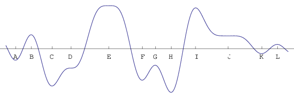

Fourier did not think all critical point were equally interesting. For example, critical point is not particularly interesting: by Rolle’s theorem there has to be a critical point between the zeros on either side of , so there is nothing special about the point . Similarly, none of , , , , , , or is interesting to Fourier. The remaining critical points are interesting: , , and because in addition to vanishing, so do some additional derivatives, so those points contribute “extra” zeros to ; and point is interesting because it is a negative local maximum, which is not predicted by Rolle’s theorem. Table 5.1 compiles information about the behavior at each critical point. The entries , , and refer to the function being positive, negative, or zero; a means a nonzero value (which could be positive or negative; and a blank entry means the value is irrelevant in terms of Fourier’s classification of critical points.
| 0 | 0 | ||||||
| 0 | 0 | ||||||
| 0 | 0 | ||||||
| 0 | 0 | 1 | |||||
| 0 | 0 | 0 | 1 | ||||
| 0 | 0 | ||||||
| 0 | 1 | ||||||
| 0 | 0 | ||||||
| 0 | 0 | ||||||
| 0 | 0 | 0 | 0 | 2 | |||
| 0 | 0 | ||||||
| 0 | 0 |
The final column of Table 5.1 is a number that expresses how “interesting” the critical point is, in Fourier’s view. More specifically, is the number of “extra” zeros that has arising from the point , where by extra we mean “more than one would expect only from Rolle’s theorem.” The extra zeros might be at , which happens at , , and . Or they might be nearby: the second extra zero from is either or , although it is not meaningful to specify which one it is.
Looking at the plots in Figure 5.1, we see that has 9 real zeros in that interval, so by Rolle’s theorem should have at least 8 real zeros in that interval. We can count that actually has 18 real zeros counting multiplicity (because has multiplicity 2, has multiplicity 3, and has multiplicity 4). There are 10 extra zeros, which is twice the sum of the values of in Table 5.1.
Another interpretation of is that it is the number of pairs of complex conjugate zeros of which are needed to explain the funny business at the critical point .
To relate to our earlier discussions, if , then either or or has a non-negative minimum or non-positive maximum at .
Here is a formula for . Suppose is a critical point which is not a zero of , and furthermore suppose
| (5.1) |
and . That is, exactly the first derivatives of vanish at . Then
| (5.2) |
That formula agrees with the values in Table 5.1, and we leave it as an exercise to check the other cases. We set if is identically zero, or if is not a zero of , so is defined for all , but it is for almost all . We will call the Fourier multiplicity of the critical zero of .
Now we assemble the above ideas into Fourier’s proof of Theorem 2.2, introducing two new functions which help us keep track of the quantities of interest. First is the function which adds up all of the Fourier multiplicities of :
| (5.3) |
The sum is over all complex numbers , but recall that for all but finitely many , so really it is a finite sum.
We use to express an observation we made earlier. Since counts the number of pairs of non-real zeros of which are causing the funny business near in the graph of , we have:
| (5.4) |
The factor of of the right of (5.4) comes from the fact that counts pairs of non-real zeros. As a formula, , where counts the number of non-real zeros of the nonzero polynomial (if is identically zero, we set ). That was Fourier’s key insight into the proof of Theorem 2.2. Rearranging and then using induction, we have
| (5.5) | ||||
| (5.6) | ||||
| (5.7) | ||||
| (5.8) |
for any .
If is larger than the degree of then is identically zero so and we have . If does not have all real zeros, then , so for some . But that implies at least one of , , or has a non-negative minimum or non-positive local maximum. That completes Fourier’s proof of Theorem 2.2.
The reader is invited to locate where in Fourier’s proof we used the fact that the roots of are distinct.
6. Infinitely many zeros
A question on MathOverflow [5] asked about an equivalence to the Riemann Hypothesis stated in the official description [1] of the Riemann Hypothesis Millennium Problem:
The Riemann hypothesis is equivalent to the statement that all local maxima of are positive and all local minima are negative, ….
Here , called the Riemann -function, is closely related to the Riemann zeta-function. See Section 6.2 for definitions and background. For this immediate discussion, it is sufficient to know that is real for real , and the Riemann Hypothesis is the assertion that all zeros of are real. So, it is similar to the real polynomials we have been discussing, except it has infinitely many zeros.
The condition for a polynomial to have only real distinct zeros involved maxima and minima of the original function, and also of all derivatives; however, the quote above does not mention derivatives. Is our understanding of polynomials giving us good intuition for functions with infinitely many zeros, and so we should be skeptical of that claimed equivalence to the Riemann Hypothesis?
As we will explain, our intuition for polynomials is very likely guiding us in the right direction. However, establishing an analogue of Theorem 2.2 for a class of functions which includes the Riemann -function, is an unsolved problem!
Understanding the similarities between polynomials and certain (but not all) functions with infinitely many zeros, and the relevance to the Riemann Hypothesis, is the topic of the remainder of this paper.
6.1. The Riemann zeta-function and the prime numbers
The Riemann -function is defined by the Dirichlet series
| (6.1) |
That series was first studied by Euler, who used it to prove that there are infinitely many prime numbers. The infinitude of primes had already been proven by Euclid, but Euler’s result is better: he showed that the series diverges. Here is the sequence of prime numbers. If the sequence of primes increased very quickly (a possibility that is allowed by Euclid’s proof), then Euler’s series might converge. Euler’s result puts limitations on how quickly the sequence of primes can grow.
Euler’s proof uses the series (6.1) for a real number. He exploits the fact that the series grows without bound as , which follows from the fact that the harmonic series diverges. But it is Riemann’s name, not Euler’s, which is attached to the -function, and rightly so. Riemann had the brilliant insight to consider for a complex number.
What does the series (6.1) mean when is not real? Let be a complex variable, where and are real variables. (The seemingly unusual choice of variable names has become standard when discussing the Riemann -function.) The exponential of a complex number is defined by Euler’s formula for . Thus,
| (6.2) |
That formula explains what the terms in the series mean for complex , but where does the series converge? For any real number we have
| (6.3) |
Thus, . Therefore, by the so-called11 1 We write “so-called” because it was a terrible idea to name a result after the variable in the expression, since the letter used for the variable is an arbitrary choice. The name “zeta test” is better. “-series test” from calculus, which we will call the “zeta test,” (6.1) converges absolutely for .
The Dirichlet series for only makes sense for , but there are other expressions for the -function, which we will not describe here, which allow us to define for all except for . At the -function has a “simple pole,” which means that as . In other words, the -function “blows up” for near , but in the nicest possible way.
Riemann discovered that the zeros of the -function encode secrets about the prime numbers. The prime number theorem is the assertion that , meaning that . Here “” means “natural logarithm.” Here is a silly proof of Euler’s theorem that diverges: combine the prime number theorem, the integral test, and the limit comparison test. That proof is silly because the prime number theorem is a deep result, and Euler’s theorem can be proven with much more mundane input.
The prime number theorem was proven in 1896 by Hadamard and de la Vallèe Poussin, independently. The key step in their proofs was showing that has no zeros on the line. Riemann knew that the -function had no zeros for . The prime number theorem followed by turning that into a non-strict inequality. That may seem like a minor improvement, but in fact it was one of the major results of 19th century mathematics.
For the remainder of this paper we will set aside connections to the prime numbers and just focus on analytic properties of the -function.
6.2. Symmetries of the Riemann zeta-function
The -function has a hidden symmetry which is revealed by the Riemann -function, defined by
| (6.4) |
Here is Euler’s Gamma-function, defined by
| (6.5) |
The integral (6.5) converges for , and one can also check that . Just as happened with the Dirichlet series for , we have an expression for which is valid for some , but we want to make use of the -function for other values of . Euler figured out how to do that. Integrating by parts (with and ) we find
| (6.6) |
which us usually written in the form (which is equivalent, because we are just renaming variables) . If we rearrange that to get , then we see that the right side is known for except for , and we can use that as the definition for the left side. Thus, we now know for , except for . Repeating the same procedure we can define for , except for or , then for , except for , , or , and so on.
Euler’s motivation was somewhat different: he used the expression to show that if is a positive integer, then . In other words, the -function provides a way of extending the factorial function to any positive real number.
Riemann showed that (6.4) defines for all and furthermore it satisfies the following surprising symmetry which is called the functional equation:
| (6.7) |
In other words, the -function is symmetric around the line . Combining the functional equation with the fact that is real when is real, we can conclude that the zeros of the -function either lie on the -line, or occur in pairs symmetrically on either side of it. The Riemann hypothesis is the conjecture, made by Riemann in 1859, that all zeros of the -function actually lie on the line. These days the line is known as the critical line.
Note that the zeros of are also zeros of , but actually has some additional zeros which are considered unimportant and go by the name trivial zeros. The Riemann hypotheses is usually stated in the form “the nontrivial zeros of the Riemann zeta function lie on the critical line.”
We are one step away from connecting to our earlier discussion on real polynomials with real zeros. We can convert to a function which is real on the real axis by a simple change of variables, creating the Riemann -function:
| (6.8) |
Here is a complex variable, and and are real. We have: is real when is real, its zeros lie either on the real line or in complex conjugate pairs, and the Riemann Hypotheses (RH) is the conjecture that all zeros of are real. It is universally believed by all experts, even those who are skeptical about RH, that all zeros of are simple. Thus, we are in a situation parallel to our discussion about real polynomials with distinct real zeros, except that has infinitely many zeros. Although we don’t know that all the zeros of are real, we do know that all zeros either are real, or they lie close to the real axis. Combining the functional equation with the fact that is nonzero for shows that all zeros of lie in the strip .
One of the magical facts about polynomials is they can be written as a product of linear factors, each factor corresponds to a zero, and the zeros determine everything about the polynomial except for a constant factor. We will see that something similar holds for certain functions that have infinitely many zeros.
6.3. Another way to factor a polynomial
Suppose is a polynomial of degree , with roots , …, . If none of the equal , then we can rearrange (2.1) to get
| (6.9) | ||||
| (6.10) |
where in the second line we used product notation, which is analogous to summation notation. If is a root with multiplicity , and , …, are the nonzero roots, then we have
| (6.11) |
The product form (6.9) is useful because it can generalize to the case of infinitely many zeros. But before going into the details, let’s consider the concept of an infinite product.
6.4. Infinite products
Infinite sums are familiar: . That sum might converge or it might diverge. It converges if the go to 0 fast enough. Otherwise, it diverges. An empty sum is defined to equal .
Similarly, an infinite product, , might converge, or it might diverge. It converges if the go to 1 fast enough. Otherwise, it diverges. The empty product is defined to equal .
The definition of convergent infinite product is analogous to convergent infinite sum, with one subtle difference:
Definition 6.1 (Convergence of an infinite product).
The infinite product
| (6.12) |
converges if there exists such that is nonzero for , and the limit
| (6.13) |
exists and is nonzero. If is the limit in (6.13), then we say that the infinite product converges to .
A possibly unexpected feature of the definition is that in a convergent infinite product, only finitely many terms can be zero, and the product of the nonzero terms also cannot equal zero. That condition becomes natural when relating infinite products to infinite sums. Taking logarithms we have
| (6.14) |
Since each in (6.14) is nonzero, and (for the infinite product to have any hope of converging) close to if is sufficiently large, its logarithm is well-defined and close to . If the limit as exists on the right side of (6.14), then the limit inside the parentheses on the left side of (6.14) exists and is nonzero. Thus, the infinite product converges if and only if the infinite sum converges.
Before looking at the convergence of some infinite products, let’s recall the geometric series
| (6.15) |
which we can integrate to obtain
| (6.16) |
A useful way to rearrange that expression is
| (6.17) |
We will use this to determine whether certain infinite products converge.
Let be any number. Does the product
| (6.18) |
converge? First: are the terms nonzero if is sufficiently large? Yes, we just need . Second, taking logarithms we have
| (6.19) | ||||
| (6.20) |
We recognize the harmonic series, which diverges, so the product diverges.
Does the product
| (6.21) |
converge? First: are the terms nonzero if is sufficiently large? Yes, we just need . Second, taking logarithms we have
| (6.22) | ||||
| (6.23) |
By the zeta test, those series converge, therefore so does the infinite product.
Does the product
| (6.24) |
converge? As in the first example above, the terms are nonzero if . When we take logarithms, the summand is
| (6.25) | ||||
| (6.26) | ||||
| (6.27) |
so by the zeta test, the sum, and hence the product, converges.
In the above discussion we have been somewhat imprecise in our use of the approximation . The issue which can arise is that just because a term is smaller, does not mean that an infinite sum involving that term will be smaller. For example, consider
| (6.28) |
The first sum on the right converges (by the alternating series test). The second sum has smaller terms (because ), but the second sum diverges because it is the harmonic series. Thus, just because terms are smaller doesn’t mean that we can ignore them. But there is a case when we can: when all the terms are positive. That motivates this definition:
Definition 6.2.
The product
| (6.29) |
converges absolutely if
| (6.30) |
converges absolutely.
The ideas in the previous discussion prove that an absolutely convergent product converges.
7. Entire functions of finite order
Polynomials are classified by their degree, or equivalently, the number of zeros counting multiplicity. There is another, also equivalent way, to classify polynomials: how fast they grow. If is a polynomial of degree , and is very large, then is approximately . In other words, if and is sufficiently large, then
| (7.1) |
We can use (7.1) as an alternate definition of the degree of a polynomial: it is the infimum (greatest lower bound) of the numbers for which (7.1) holds as .
The value of having multiple equivalent definitions is that some generalize to other contexts, and some do not. In this case, it is the rate of growth which can be used to classify functions that have infinitely many zeros.
We will consider entire functions, which means that the function has a Taylor series which converges for all . Examples are , , polynomials, as well as sums, products, and compositions of those functions. Non-examples are , , , and . A good reference for the material in this section is [4].
For polynomials there is a direct relationship between the growth of the function and the number of zeros, but for entire functions the relationship is not exact. An entire function with many zeros must grow quickly, but the function grows quickly even though it has no zeros. It turns out that is the complete story: the growth of an entire function is determined by its zeros, and by factors of the form where is an entire function. That motivates the definition of the order of an entire function.
Definition 7.1.
Suppose is an entire function, and suppose there exists a real number such that if is sufficiently large,
| (7.2) |
Then we say that has finite order. If has finite order, then the order of is the infimum of the set of such that (7.2) holds as .
Combining (7.1) and (7.2), and using the fact that grows slower than any power of , we see that polynomials have order 0.
The exponential function has order , and more generally if is a polynomial of degree then has order . Finite sums (or products) of functions of finite order have finite order, and the order of the sum (or product) is at most the order of the largest term (or factor). The Riemann -function has order 1, although that is not easy to deduce only from the information we have provided in this paper. The Euler -function is not entire because it is not defined at the negative integers, but is an entire function of order 1.
The beauty of entire functions of finite order is that they can be written as an infinite product with a nice form. This was discovered by Hadamard, as part of his proof of the Prime Number Theorem. We will state a special case which is sufficient for our needs.
Theorem 7.2 (Hadamard).
By Definition 6.2, the sum in (7.3) converges, and the same ideas we used when discussing (6.24) show that in (7.4) the sum converges. In general, for a function of order with non-zero zeros , the series converges if . Thus there is a close relationship between the order of a function and the distribution of its zeros, with low order functions having zeros distributed more sparsely.
Now we have the ingredients to extend our results on polynomials to functions with infinitely many zeros.
7.1. Zeros of derivatives
Entire functions of order less than 2 are nice because the analogue of Theorem 2.1 holds for them:
Theorem 7.3.
Suppose is an entire function of order less than 2, which is real on the real axis and has only distinct real zeros. Then all zeros of are real, and furthermore all local maxima of are positive and all local minima of are negative.
Since the derivative of an entire function of order is entire of order , the conclusion of Theorem 7.3 applies to every derivative and not only .
The proof of Theorem 2.1 used Rolle’s theorem and the fact that the derivative of a polynomial has one fewer zero than the original polynomial. However, it makes no sense to talk about “one fewer” zero of the derivative when there are infinitely many zeros. Instead, we will show that has exactly one real zero between each pair of consecutive real zeros of , and no other zeros.
Proof.
Suppose satisfies the conditions in the Theorem 7.3. Since is an entire function of order less than , it has the form (7.4). Furthermore, , , and all are real. Since , we have
| (7.5) |
Note that the series in (7.5) is defined whenever is not a zero of , and the sum converges absolutely wherever it is defined.
Suppose and are consecutive zeros of , and . We wish to show that has only one zero in that interval. Since has constant sign on that interval, this is equivalent to having exactly one zero on that interval. That function has at least one zero on that interval because by (7.5), that function is large and positive if is slightly larger than , and it is large and negative if is slightly smaller than .
To show that , equivalently , has only one zero in that interval, it is sufficient to show that is decreasing on that interval. But that follows from differentiating (7.5):
| (7.6) |
which is negative for real whenever it is defined. In particular it is negative on the interval .
We have shown that has only one zero in each interval , which proves that all maxima of are positive and all minima of are negative. Now we must prove that has no non-real zeros. In (7.5) let , and then take the imaginary part of that expression, making use of the fact that and are real:
| (7.7) |
That is nonzero if , because every term is nonzero and has the same sign, therefore cannot be if is not real, because its imaginary part is not zero. ∎
The above proof is not quite right. The first two paragraphs implicitly assumed that the zeros of range from to , but that might not be the case: there might be a largest, or a smallest, zero, or there might only be finitely many zeros. We leave it as an exercise to work out the details for those cases. Illustrative examples to consider are where is a real polynomial.
7.2. The converse
Does the analogue of Theorem 2.2 hold for entire functions of order less than 2? Definitely not. The function real on the real line and is entire of order . It has zeros at for all , so it has infinitely many complex zeros. But it has no real maxima or minima. Its first derivative, and every higher derivative, is , which also has no real maxima or minima.
All is not lost: our motivation was the Riemann -function, which has order 1 and is real on the real axis. It has one more key property: its complex zeros, if they exist, must have imaginary part between and , which follows from the fact that has no zeros in . That is, all zeros lie in a strip around the real axis. The counterexample has zeros arbitrarily far from the real axis. Maybe the analogue of Theorem 2.2 holds for functions with all zeros near the real axis?
Y-.O. Kim [3] proved a version with that extra assumption, plus an additional extra assumption.
Theorem 7.4.
Suppose is an entire function of order 1 which is real on the real axis and has all zeros in the strip for some . Let be the non-real zeros of and further suppose
| (7.8) |
If and all of its derivatives have every maximum positive and every minimum negative, then has only real zeros, and all zeros are distinct.
In other words, if the zeros are in a strip and there are not too many complex zeros, then the analogue of Theorem 2.2 is true.
Might Theorem 7.4 be true without the extra condition on the non-real zeros? Or maybe if there are many non-real zeros, they can somehow conspire to stay away from the real axis as the function is differentiated? Those are research questions.
One could apply Theorem 7.4 in its current form, of one could show that the Riemann -function had sufficiently few non-real zeros. This is far beyond the realm of possibility in the foreseeable future. At present it has not even been shown that at least half of the zeros of the -function are real.
At the start of this section we asked whether there might be an equivalence to the Riemann Hypothesis that only involved the maxima and minima of the -function and its derivatives. Such an equivalence cannot follow from a general statement about real entire functions of order 1, as illustrated by the example and . That function has zeros at and all other zeros are real. As increases, the real zeros move closer together but the pair of complex zeros do not move. If is small, the function has a positive local minimum, but if is large enough, it does not. As increases, it takes more and more derivatives before a positive local minimum or negative local maximum appears. That is a another version of a lesson from Figure 1.1: funny business comes from complex zeros, complex zeros close to the real axis cause more funny business, and closeness to the real axis should be measured relative to the gaps between nearby zeros.
References
- [1] E. Bombieri, Problems of the Millennium: the Riemann Hypothesis, available at https://claymath.org/sites/default/files/official_problem_description.pdf linked from https://claymath.org/millennium-problems/riemann-hypothesis . Accessed online, October 16, 2020.
- [2] Marc Chamberland, When Are All the Zeros of a Polynomial Real and Distinct?, American Mathematical Monthly 121:1, August 30, 2019.
- [3] Y.-O. Kim, Critical points of real entire functions and a conjecture of Pólya, PAMS, Vol. 124, No. 3, (1996), 819-829.
- [4] B. Ya. Levin, Lectures on entire functions. Translations of Mathematical Monographs, 150. American Mathematical Society, Providence, RI, 1996. xvi+248 pp. ISBN: 0-8218-0282-8
- [5] MathOverflow website: On a Possible equivalent of Riemann Hypothesis, https://mathoverflow.net/questions/339863/on-a-possible-equivalent-of-riemann-hypothesis . Accessed online, October 16, 2020.