Exploiting Angular Multiplexing for Polarization-diversity in Off-axis Digital Holography

Space-division multiplexing (SDM) has the potential to extend the capacity of optical fibers greatly beyond what is possible with current single-mode technologies. SDM uses spatially-diverse fibers such as few-mode, multi-mode, multi-core, coupled-core, and few-mode multi-core fibers, for which multiplexer devices to couple in to these fibers are required. For the development of these multiplexers such as photonic lanterns (PLs) [1], proper characterization tools for important metrics such as cross-talk (XT) and mode-dependent loss (MDL) are very desirable.

Characterization of SDM systems and devices can be done by methods such as analysis of equalizer taps[2] through which system-level metrics can be obtained, whilst optical vector network analysers (OVNAs) [3, 4] are also able to extract some valuable device-level metrics. Off-axis digital holography (DH) [5], however, provides access to the full complex optical field for all device inputs and has recently been used to measure a plethora of SDM devices[6, 7, 8, 9]. To access both polarizations of the optical field, DH is performed separately on each polarization, either by using multiple near-infrared (NIR) cameras or by using a different part of the camera, essentially multiplexing polarizations spatially. Alternatively, in the imaging field of research[10, 11, 12], the same part of a camera was used to perform DH on a signal using two orthogonally polarized reference beams which were separated in angle, essentially multiplexing polarizations angularly.

In this work, we introduce angular multiplexing to achieve polarization-diversity in DH as an alternative to spatial multiplexing for measurements of the complex optical field and transfer matrix of an SDM device. Both spatial and angular multiplexing schemes are discussed and compared through measurements of the same PL. Similar XT values of $13.8\text{\,}\mathrm{d}\mathrm{B}$ and $14.0\text{\,}\mathrm{d}\mathrm{B}$ are measured using spatial and angular multiplexing, respectively. Furthermore, we find very similar values of $1.50\text{\,}\mathrm{d}\mathrm{B}$ and $1.45\text{\,}\mathrm{d}\mathrm{B}$ for MDL, confirming angular multiplexing is a viable alternative to spatial multiplexing. Angular multiplexing may lead to a simpler optical setup with fewer components in the signal path and greater magnification of the signal beam, increasing the resolution of measured optical fields.

Fig. 1 shows a commonly-used DH setup where spatial multiplexing is used to achieve polarization-diversity. A 4f optical setup coherently combines signal $1550\text{\,}\mathrm{n}\mathrm{m}$ laser light with $100\text{\,}\mathrm{k}\mathrm{H}\mathrm{z}$ linewidth from a device-under-test (DUT), in this case a PL, with slightly angled (<5 degrees) reference light, producing a fringe pattern on a NIR camera. Note that the lens setup is not drawn to scale to conserve space. A Wollaston prism with a 20 degree beam separation splits polarizations spatially across the camera, and optical switches are used to address all input ports and polarizations of the DUT.

In contrast to the spatial multiplexing scheme of Fig. 1, Fig. 2 shows the use of the entire camera surface for both polarizations through angular multiplexing. Instead of splitting light from both polarizations spatially, two orthogonally-polarized reference beams are used, each at a different slight angle with respect to the signal, making two different overlapping fringe patterns appear on the camera, which can be separated digitally. Fewer optical components are required in the signal path and potentially larger beam widths lead to greater flexibility.

The main elements of the DH signal processing chain are depicted in Fig. 3 for measurements obtained using the spatial multiplexing setup detailed in Fig. 1. Since the fringe patterns corresponding with the X- and Y-polarization are spatially separated on the NIR camera, they can be cropped from frame and processed separately.

For each polarization, the intensity of the fringe pattern can be described by Eq. 1. Both cropped images from the spatial domain are Fourier transformed to the angular domain. The detection of the signal and reference directly, $|S|^{2}$ and $|R|^{2}$, end up at DC in the angular domain since there is no angle between the signal or reference with respect to itself. The beating between signal and reference, the fringe pattern in the spatial domain, $SR^{*}$, however, manifests itself as a distinct part in the angular domain, with significant separation from DC-terms, which can be cropped in the angular domain to extract the desired term of Eq. 1. It is inversely Fourier transformed, revealing the complex $SR^{*}$ term in the spatial domain, both in amplitude and phase, even though the camera only measures intensity. Given the reference is by approximation a plane wave, $SR^{*}$ equates to $S$, which, after processing both polarizations, results in the full polarization-diverse complex optical field for a given device excitation. Repeating the measurement for all possible input states through the optical switches in Fig. 1 provides the complete description for the device for a given wavelength.

Additional processing provides further insight. The optical fields can be digitally demultiplexed to any desired modal basis using overlap-integrals, providing a transfer matrix between device input port and polarization and spatial mode of the desired modal basis. Important performance metrics such as XT and MDL can be obtained through analysis of this transfer matrix. Note that the desired modal basis can be any, for example a specific optical fiber of interest, essentially predicting how the device would behave when coupled or spliced with that specific fiber.

The intensity of the camera frame in Fig. 4 for the angular multiplexing setup of Fig. 2 can be described by Eq. 2. Cross-terms between X- and Y-polarizations are omitted since perfectly orthogonally-polarized beams do not interfere. In the spatial domain, both polarizations overlap, but after a fast Fourier transform (FFT) they are separated in the angular domain since reference beams $R_{X}$ and $R_{Y}$ are placed under a slight angle, both with respect to the signal and each other. Since $S_{X}R_{X}^{*}$ and $S_{Y}R_{Y}^{*}$ are separated in angular domain, similar to the signal processing chain for spatial multiplexing, they can be cropped and inversely Fourier transformed separately to reveal the complex optical field in spatial domain for both polarizations. The extracted fields are the same for spatial and angular multiplexing if the polarization axes of the two reference beams of the angular multiplexing setup are aligned to the Wollaston prism of the spatial multiplexing setup. Note that some interference between the orthogonally-polarized reference beams, $R_{X}R_{Y}^{*}$, is observed in the angular domain of Fig. 4, indicating they were not perfectly orthogonal.

The same PL was measured using both the spatial and angular multiplexing scheme for each of input ports and polarizations, and one complex optical field per output polarization is extracted using the signal processing techniques detailed in the previous section. Two of these output fields when port 3 polarization X was excited are displayed as an inset in Fig. 3 and Fig. 2 for spatial and angular multiplexing, respectively. The intensity of the image represents the amplitude of the optical field whilst a cyclic colormap is for the phase. It is observed that the extracted fields look very similar for both measurement setups. The extracted fields, 12 per measurement, look very similar for both multiplexing techniques, but are omitted in this paper to conserve space. This qualitatively confirms the validity of the angular multiplexing scheme by comparing it to the tried-and-tested spatial multiplexing setup.

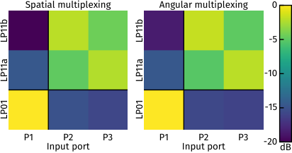
To quantitatively assess the measurement results, the extracted fields are digitally demultiplexed to the Hermite-Gaussian linearly polarised (LP) modal basis. The resulting 6x6 complex transfer matrix can be condensed to a 3x3 power transfer matrix, from input port to output LP-mode, which is depicted in Fig. 5 for both spatial and angular multiplexing. Mode-group XT is evaluated using this matrix and equates to $-13.8\text{\,}\mathrm{d}\mathrm{B}$ and $-14.0\text{\,}\mathrm{d}\mathrm{B}$ for spatial and angular multiplexing, respectively. MDL, calculated through singular value decomposition of the 6x6 complex transfer matrix, is $1.50\text{\,}\mathrm{d}\mathrm{B}$ and $1.45\text{\,}\mathrm{d}\mathrm{B}$ for spatial and angular multiplexing, respectively. Therefore, quantitatively, both measurement schemes reveal similar performance metrics for the same device, further validating the concept of angular multiplexing for polarization-diverse DH.

These results are achieved using many of the same optical components for the spatial and angular multiplexing setup. However, in principle, the angular multiplexing scheme may benefit from using different components. For example, since no Wollaston prism is required, the reference beam width may be increased so it better resembles a plane wave. Also, since a larger area of the camera is available, greater magnification in the 4f lens setup can increase the number of pixels used for the signal and therefore increase resolution and dynamic range of the extracted optical fields. On the other hand, by incorporating two fringe patterns on the same part of the camera, dynamic range is reduced.

Furthermore, one of the key attractions to DH as a measurement technique is the low amount of optical components required to capture the signal light, keeping the influence of aberrations minimal. Thus it might prove beneficial that the angular multiplexing scheme does not have the Wollaston in the signal path, and only introduces a simple beam-splitter in the reference path.

Finally, some interference between both reference beams is observed in Fig. 4, which could give meaningful insight in the reference beam amplitude and phase, potentially for correction of its deviation from a perfect plane-wave.

Angular multiplexing is introduced as a more flexible alternative to spatial multiplexing for polarization-diverse digital holography measurements of space-division multiplexing devices. Both techniques are used to measure the same photonic lantern to test the novel angular scheme against the tried-and-tested spatial multiplexing scheme. Similar values are measured for mode-group cross-talk, $-13.8\text{\,}\mathrm{d}\mathrm{B}$ versus $-14.0\text{\,}\mathrm{d}\mathrm{B}$, and mode-dependent loss, $1.50\text{\,}\mathrm{d}\mathrm{B}$ versus $1.45\text{\,}\mathrm{d}\mathrm{B}$, using spatial and angular multiplexing, respectively. Therefore, angular multiplexing for polarization-diverse digital holography measurements is a valid alternative.

Partial funding from the NWO Gravitation Program on Research Center for Integrated Nanophotonics (Grant Number 024.002.033) and by TU/e-KPN Smart Two project.

References

- [1] Amado Vel“’azquez-Ben“’tez et al. “Scaling photonic lanterns for space-division multiplexing” In Scientific reports 8.1 Nature Publishing Group, 2018, pp. 8897
- [2] Peter Winzer and Gerard Foschini “MIMO capacities and outage probabilities in spatially multiplexed optical transport systems” In Optics express 19.17 Optical Society of America, 2011, pp. 16680–16696
- [3] N.. Fontaine et al. “Characterization of space-division multiplexing systems using a swept-wavelength interferometer” In OFC, 2013 DOI: 10.1364/OFC.2013.OW1K.2
- [4] Simon Rommel et al. “Few-mode fiber, splice and SDM component characterization by spatially-diverse optical vector network analysis” In Opt. Express 25.19 OSA, 2017, pp. 22347–22361 DOI: 10.1364/OE.25.022347
- [5] Martin Pl“”oschner, Tom“’as Tyc and Tom“’as Cizm“’ar “Seeing through chaos in multimode fibres” In Nature Photonics 9.8 Nature Publishing Group, 2015, pp. 529
- [6] Nicolas Fontaine et al. “Laguerre-Gaussian mode sorter” In Nature communications 10.1 Nature Publishing Group, 2019, pp. 1865
- [7] M. Mazur et al. “Characterization of Long Multi-Mode Fiber Links using Digital Holography” In OFC, 2019
- [8] Sjoerd van Heide et al. “Low-loss Low-MDL Core Multiplexer for 3-Core Coupled-core Multi-core Fiber” In 2020 Optical Fiber Communications Conference and Exhibition (OFC), 2020, pp. 1–3 IEEE
- [9] Juan Alvarado-Zacarias et al. “Assembly and Characterization of a Multimode EDFA Using Digital Holography” In Optical Fiber Communication Conference, 2020, pp. Th1H–6 Optical Society of America
- [10] Tristan Colomb et al. “Polarization imaging by use of digital holography” In Applied optics 41.1 Optical Society of America, 2002, pp. 27–37
- [11] Caojin Yuan et al. “Resolution improvement in digital holography by angular and polarization multiplexing” In Appl. Opt. 50.7 OSA, 2011, pp. B6–B11 DOI: 10.1364/AO.50.0000B6
- [12] Takanori Ochiai et al. “Angular multiplex recording of data pages by dual-channel polarization holography” In Opt. Lett. 38.5 OSA, 2013, pp. 748–750 DOI: 10.1364/OL.38.000748