Multi-field inflation from a higher derivative Supergravity model
Abstract
We study the cosmological evolution of a supergravity model, dual to a higher derivative supergravity model coupled to scalar fields so that in the Einstein frame the model is ghost free. We find that this model admit slow roll inflationary solutions showing essentially two-field inflation. The cosmological parameters calculated for this model lie in acceptable range with corrections of the order , N being the number of e-foldings, compared to the Starobinsky inflation model.
I Introduction
The study of gravity theories including higher order terms of the curvature and its derivatives is well motivated since in the effective theory of gravity such terms are present Buchdahl; tHooft:1974toh; stelle1978. The treatment of these theories is for many purposes facilitated by the fact that they admit a dual description in terms of Einstein gravity coupled to a certain number of scalar fields whitt; Wands; SOTIRIOU; CAPO. The above property and the corresponding dual description has been extended to supergravity models THEISEN; CECOTTI. The major problem for the use of the dual formulation in the study of these higher order theories is that the scalar fields necessarily introduced do not correspond to physical degrees of freedom leading thus to ghost states. This happens inevitably departing from quadratic terms in the curvature tensor and even in special cases of quadratic generalization of the Einstein gravity. Several attempts to deal with this problem and to construct ghost free models have been presented in the bibliography GHOST; BISWAS1; BISWAS2. Certainly the study of the dual description in an attempt to understand the effect of higher order terms coming from quantum corrections has to do with the short distance behaviour of gravity. Interestingly enough the extra mode arising in a theory and in its supersymmetric extension seem to be relevant for cosmology since in the dual description one of the corresponding scalar fields is responsible for the inflationary behaviour as is recognized in the celebrated Starobinsky’s model. The above reasons justify both the history which goes many years back and the recent revival of the study of generalizations of the Einstein (super)gravity.
In a relatively recent work a supergravity model has been presented with highest order terms of the form and . Allowing kinetic terms for the chiral multiplets needed to be introduced in the higher order description the auxiliary fields become dynamical. In this way the physical degrees of freedom match, leading to a ghost free dual form of Einstein supergravity coupled to four chiral multiplets. Furhermore a preliminary discussion of the cosmology of this model was performed, resulting to deformation of the Starobinky’s model STAR. In particular the potential has directions reminiscent of the Starobinsky model but in the cosmological evolution at least two fields are relevant. Modifications of the Starobinsky inflation from generalized gravity models are also addressed in the literature Cuzinatto2018. In this work we perform a detailed analysis of this model with the following order. In the next section we give a very short review of the model in discussion. In Sec. III we perform the analysis of the cosmological evolution pointing out that from the eight real scalars involved, only two are essential for the evolution, while six of them relax very quickly to their minimum value. In Sec. IV we calculate the basic cosmological parameters following the literature on multifield inflation Mukhanov1990; Seery2005; Kim2006; Kaiser2012; Kaneda2015. In particular corrections of the order , denoting the number of e-foldings, to the Starobinsky model are found keeping this generalization viable. We conclude with the discussion in Sec. V. Many of the details of our analysis are presented in the two Appendices that close the work.
II Setting the model
The model under consideration is analysed in its basic characteristics in Diamandis2017. It is a higher supergravity model described by the following functions of chiral superfields,
| (1) |
with the specific choices for ,
| (2) |
where are assumed to be positive.
The pure gravitational part in the higher description is given by
| (3) |
It is known that supergravity models admit a dual description as Einstein gravity models which have ghost states for CECOTTI. In the work mentioned above it was proven that no ghost-states appear in the ordinary supergravity description at the cost of keeping coupling of certain scalar modes in the higher description equalizing thus the physical degrees of freedom in the two descriptions. This was achieved via the introduction of the and the terms in the function .
At the Einstein frame of supergravity description of the above model the action is determined by the Kähler function
| (4) |
and if we name the fields collectively as with the action is given by
| (5) |
where is the spacetime metric, its determinant, the Ricci scalar and
| (6) |
the metric in the field space with the indices running over the four complex scalar fields.
The potential is given by
| (7) |
where
Furthermore, in that work it has been showed that the potential becomes stable with the addition of a stabilizer term proposed in Kallosh2013 to the function and provided that the function is at most quadratic in of the form
| (8) |
with real coefficients11 1 Consideration of more general functions of may be implemented by introducing additional stabilizing term e.g. but such an option is not examined in this work. . Then the potential has a global minimum with vanishing vacuum energy at . Note also that the following resrtictions
| (9) |
ensures the absence of tachyonic states.
III Cosmological evolution
In order to study the cosmological behaviour of the model resulting from (5), with the inclusion in of the term and given by (8), we assume a Friedmann-Robertson-Walker metric
| (10) |
and separating the fields into real and imaginary parts, we reparametrise our model in terms of eight real fields denoted by with . The field equations read
| (11) |
where and the Hubble parameter is given by
| (12) |
The fields relevant for the study of the cosmology are , while the remaining six fields will be considered to relax to their zero minimum value. In particular in the Appendix A it is shown that these fields tend rapidly to their minimum value leaving the fields to drive the cosmological evolution of the model. Being restricted in the space of these two fields the potential reads
which is a positive semidefinite function and reparametrising as and the corresponding metric becomes 22 2 It is easily checked that either setting the fields to their minimum value in the set of the full equations in (11), or working with the restricted lagrangian, leads to the same set of equations to be studied.
| (14) |
The metric can be brought into diagonal form if we set 33 3 From now on we take which is necessary in order to have canonically normalized Einstein gravity in the dual description, see Diamandis2017.
| (15) |
The choice of the constant in the normalization of will be explained later on. In the above basis the metric elements become
| (16) |
and the potential gets the form
| (17) |
with
| (18) |
with the constant .
As is already mentioned the potential is positive apart from the global minimum at or equivalently at and possibly along the direction and the limit , where the potential tends to the value
| (19) |
and by demanding it to be zero, it has real solutions for only if . In order to exclude this case we shall take from now on 44 4 An inflation scenario of hill-top form is not considered in this work. . As we will see later for large number of efoldings the field takes the value or equivalently during inflation. The fine tunning case means there is no asymptote value for or during inflation and this case needs special treatment which we have not done in this work.
III.1 Evolution of the fields
The behaviour of the solutions is understood analytically although the full solution can be obtained only numerically. Since we are interested for trajectories initiating away from the minimum of the potential we consider the equations for small (large negative ). The equations of motion for the fields at lowest order in read in this case:
| (20) |
with the constants being positive and denote now the Christoffel symbols in the space of the fields . The equations for and are written in the lowest non-linear approximation.
Adopting the iteration method for the solution of the non-linear equations and starting from the linear part of the equation in eq.(20), that is from the three first term we see that they give a solution for which has a negligible contribution to the equation above. So to zero order in we get:
| (21) | |||||
Clearly the quantity as and therefore both exponents are negative 55 5 Note that if we set we may have an acceptable hill-top scenario even for . Consequently, the field settles down to values near for small . Note that the factor in the definition of in (15) is chosen so that becomes the asymptotic value for the minimum of the potential in the direction for small . In the following Figure (1) we show the evolution for the fields for some representative values of the parameters of the potential and different initial values for .
The numerical results confirm the above analytical consideration. The field is driven towards the minimum in the direction which for very small is at . This indicates that in the plane there is a trajectory perpendicular to which the potential is convex and forces the fields to follow this trajectory. In order to find the trajectory which the fields follow after they stabilize their motion we use the Hamilton-Jacobi equation, derived from the field equations,
| (22) |
Expanding it in powers of according to the Frobenius-Fuchs method
| (23) |
we find that the starting power of the expansion (23) must be or . However, for a trajectory that starts at , for the kinetic term is much larger than (the kinetic term starts in an expansion in with a negative power of , whereas the potential with a constant) and therefore it seems that we don’t have a slow roll inflation which demands . Nevertheless the numerical solution shows that even this case leads, after a few e-foldings, to slow roll evolution although it is not easy to be proven analytically.
If we restrict the expansion (23) to which obviously satisfy the slow-roll condition we obtain an ordinary power series.
Inserting the expansion in (23) in the Hamilton-Jacobi equation and furthermore expanding the functions involved in series in around , which is an attractor for , we can calculate the quantities . Furthermore expanding as
| (24) |
we can solve the equation of the trajectory
| (25) |
using the coefficients that we have calculated from the Hamilton-Jacobi equation.
The result is
| (26) |
and for the velocities for small :
| (27) |
with
| (28) |
The form of this trajectory is also confirmed from the numerical solutions with the mere assumption that the initial conditions imposed are far from the minimum of the potential as is the case for the cosmological study of the model.
IV Calculation of the number of e-foldings and of cosmological parameters
In this subsection we summarize the results concerning the cosmological parameters leaving the details which are presented in Appendix B. We will use the trajectory found in the previous subsection as it is an attractor for all the trajectories that start at asymptotic values of and . This is necessary in order to have the required high number of e-foldings. The number of e-foldings with the redefinitions
and (the already defined)
is given by:
| (29) | |||||
with ,
The values are the pivot values of the fields and are the values of the fields where inflation ends.
For later use we can also express as a function of using the expansion for large :
| (30) |
Substituting it in (29) and equating the equal powers of we get
| (31) |
The slow roll matrix is given by Seery2005:
| (32) |
If we are restricted in the fields , after the substitution all elements are only functions of and are of lowest order i.e. and are therefore small for small . The slow roll parameter is defined as and comes out to be with the redefinitions :
| (33) | |||||
being also small for where inflation occurs.
As far as the spectral index and the tensor to scalar ratio are concerned we remind that in our case we have eight real scalars, and although six of them take quickly the zero value, the perturbations of the metric and the fields in these directions have to be taken into account, as in principle they may affect the cosmological observables. In Appendix A we prove that they don’t play any role in the cosmological observables . In Appendix B we repeat the formulation described mainly in Lalak and vandeBruck for the calculation of for the case of two field inflation.
IV.1 Spectral index
The spectral index is defined in terms of the power spectrum by
| (34) |
at . Note that so
| (35) |
The result, keeping the leading and subleading term, with calculated in Appendix B in (152) and using (27) for the time derivative of , is:
| (36) |
With the substitutions and with (with the Euler-Mascheroni constant) for reads:
| (37) |
Substituting as a function of the number of e-foldings by (30) we get
| (38) | |||||
IV.2 Tensor to scalar ratio
The tensor power spectrum is given by Stewart1993
| (39) |
with .
Keeping the leading and subleading term in , we have
| (40) |
and by taking the ratio with given by (152) we get
| (41) |
Substituting as a function of the number of e-foldings by (30) the result reads
| (42) | |||||
For the determination of we require the absolute value of (which is defined as with defined in (95)) to be smaller than unity, therefore 66 6 The results are not sensitive in different way of determining .
| (43) |
with The eq. (43) has a solution for For we require as an estimation for where inflation ends
| (44) |
Then the cosmological parameter can be written for :
| (45) | |||||
and for
| (46) | |||||
The tensor to scalar ratio can be written for
| (47) | |||||
and for :
| (48) | |||||
In figure (2) we plot given by eqs (45)-(48) as a function of the number of e-foldings and of the parameter and we show indicatively the physical region dictated by observations Planck; WMAP; BICEP2; Ade2015 for and the number of e-foldings .
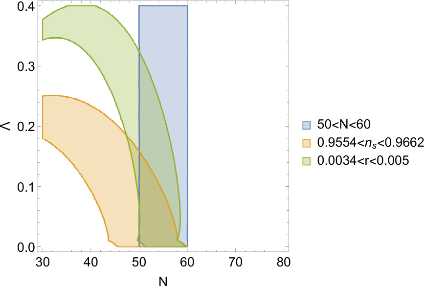
We observe that the maximum allowed value of is and that the tensor to scalar ratio is small, , typical for the Starobinsky model. Concluding we have an in principle viable model giving small deviations from the original one field inflation Starobinsky model.
V Summary - Conclusions
In this work we make a detailed study of the properties regarding the inflationary behaviour of a supergravity model. This model involves four chiral multilpets and it is dual to higher order supergravity containing and terms. These terms are purely gravitational and of order, where is the gravitational coupling constant. Despite the fact that there is a qubic term in the scalar curvature, its dual description is ghost free. This happens since in the higher order description gravity remains coupled to certain complex scalar fields and notably to one of the auxiliary fields of the chiral multiplets maching thus the physical degrees of freedom between the two descriptions. This occurs by including in the Lagrangian kinetic terms for the chiral mutiplets which cease from being just Lagrange multipliers.
The basic features of the cosmology derived from this model are the following. From the eight scalar fields involved, only two are crucial for the cosmological evolution, under very mild and natural conditions. There are solutions exhibiting slow roll behaviour in which two fields take part while the rest relax almost immediately to their minimum value. The resulting evolution certainly suggests relation to the existence of attractors studied in the bibliography Kallosh2013; Galante2014; Achucarro2017; Iarygina2018; Christodoulidis20191; Christodoulidis2019, although the precise connection is not explored in this work. Furthermore perturbations of these fields do not affect considerably the cosmological parameters. From the calculation of the cosmological parameters it turns out that the leading order correction to the result from the Starobinsky model, which is phenomenologically viable, is of order where N is the number of e-foldings. Therefore the generalization considered yield reasonable results regarding the slow roll inflation and the cosmological parameters evaluated from this.
Concluding two remarks are in order. The first has to do with the fact that the requirement for a stable potential led to consider the function to be quadratic in . For general we expect that a term of the form in the Kähler function is adequate to stabilize the potential as is the case with the term introduced by Kallosh for the chiral field . Note that such terms exist in the effective Kähler function. The sign of the coefficient may lead to stability or further instability. The second remark concerns the scalar fields required to work in the dual description. We have seen that only two of them are crucial for cosmology that is they have to do with the long range behaviour of the model. We expect that this feature holds if we consider even higher order terms of the effective action. That is, although in the Einstein frame in fact a large number of scalar fields are present, only few of them are crucial for cosmology and the majority have to do with the ultraviolet behaviour of the theory. Certainly definite answers in favour or against the above claims need much further work.
Acknowledgements
This research has been financed by NKUA ( National Kapodistrian University of Athens ). The authors wish to thank A. B. Lahanas and V. Spanos for illuminating discussions.
Appendix A Determining the degrees of freedom essential for cosmology.
In this appendix we show that the cosmologically relevant fields are the two fields while the six fields obtain very quickly zero value. If we linearize the system of equations (11) towards the six fields we obtain equations of the form
| (49) |
and defining , we have the first order equations
The real parts of the eigenvalues of the matrix are negative for in the regime , with defined in (15), if we consider as plausible values for the velocities those given by the slow roll motion with on the plane spanned by (all other fields equal to zero). Then the eigenvalues are
| (57) |
The existence of such eigenvalues at the linearized level guarantees, according to Picard’s iteration method, an iterative solution of the full system with each term in the iteration procedure converging even faster than the linear one.
The numerical analysis indicates that the condition imposed is not necessary for the eigenvalues to have negative real parts although this is difficult to be shown analytically for the full case. Nevertheless it can be shown in a reduced case where are taken to be zero. Note that this is the case already in the supersymmetrization of the Starobinsky model. In this case the matrices , are diagonal and as is can be easily seen negative definite with the mere condition adequate for the asbsence of tachyonic fields which is already imposed. The equation determining the eigenvalues of the reduced matrix is equivalent to solve three quadratic equations
where the negative diagonal elements of the matrices , correspondingly. Obviously the solutions of the above equations have negative real parts.
Next we pay attention on how perturbations of the fields may affect the power spectrum of the curvature perturbations. Starting from the action
| (58) |
with respect to we get the equations of motion
| (59) |
with the Christoffel symbol in field space. Following Kaiser2012 we perturb each scalar around its background value
| (60) |
and correspondingly the metric around the FRW metric Mukhanov1990; Bassett2005; Malik2008
| (61) |
We then consider linear perturbations of and introducing the gauge-invariant Mukhanov-Sasaki variables Mukhanov1990; Bassett2005; Malik2008
| (62) |
eq. (59) splits into background and perturbation equations
| (63) |
where denotes the covariant derivative in the field space and
| (64) |
with the curvature tensor in this space.
If we define and the unit vector along the background orbit
| (65) |
and
| (66) | |||
| (67) |
denoting the vectors in the perpendicular directions we get
| (68) |
and
| (69) |
Furhtermore the relations
| (70) |
hold meaning is perpendicular to the plane spanned by In our case because lie on a steady plane of the coordinates (or equivalently of ) and therefore the variation with time of lies on that plane also.
Using the above relations the equations of motion for the adiabatic (parallel)
and the entropy (perpendicular )perturbations
become
| (71) |
and
| (72) |
correspondingly. Note that denote the projection of the fields along the six directions in which the background fields take zero value. The reduced metric in this space is .
We note that where is the Bardeen potential Bardeen and this term is neglected if (we work in the super-horizon limit). Furthermore we observe that if and , then the fields don’t affect the evolution of and . This is the case in our model since we have already discussed that as the vectors lie on a steady plane along the motion. However the matrix has zero elements for along these directions. Therefore and the six fields don’t affect the entropy perturbations which on their turn affect the adiabatic perturbations. Therefore, the power spectrum of the curvature perturbations is not affected by the perturbations of the six fields .
Appendix B Calculation of the spectral index and tensor to scalar ratio
B.1 The power spectra
In this Appendix we follow closely and repeat for completeness the formulation in Byrnes2006; Lalak, applied in the pertinent model. We note that the action of our model can be cast in the form
| (73) |
with the redefinition
| (74) |
and then the background motion of the fields is given by
| (75) |
and the Friedmann equations read
| (76) |
We will study the perturbations in the longitudinal gauge in which the perturbed metric is given by
| (77) |
and the scalar fields are perturbed as
| (78) |
The study is mainly performed in the ”rotated” basis
| (79) |
where
| (80) |
and in the gauge invariant Mukhanov-Sasaki variables Mukhanov1990; Bassett2005; Malik2008, defined by
| (81) |
In this basis the background equations become
| (82) |
and the perturbations can be written as
The coefficients are given by
| (94) |
where we have used the fact that for our model and and
| (95) |
with
| (96) |
the adiabatic and entropy ”vectors” in field space. Also with the substitutions and the equations (B.1) read in conformal time , defined by :
where
In the slow roll approximation we have
| (106) |
Furthermore, using the exact relation , and the quantity up to order is given by
| (107) |
and up to order is given by
| (108) |
with
and .
The above system is of the form
| (119) |
with and determined appropriately from (B.1). Introducing a time-dependent orthogonal matrix which satisfies and with the change of variables we obtain
| (120) |
The matrix is quadratic in the slow roll parameters in so it is much smaller than Furthermore and since the slow roll parameters in vary very slowly with time therefore we get
| (121) |
Then the part apart from the part proportional to the identity matrix contains
which is a symmetric matrix and can be diagonalized by a matrix at Hubble crossing
yielding
We note that in our model:
| (131) |
and therefore
so .
By introducing around Hubble crossing
| (135) |
the system of equations (120) decouple and become
| (136) |
with
| (137) |
The solution of (136) with the appropriate asymptotic behaviour is
| (138) |
where is the Hankel function of the first kind of order, and the are two normalised Gaussian random variables.
By the regular definition of the power spectra
| (139) |
and the independence of variables we have
| (140) | |||||
| (141) | |||||
| (142) |
where we substitute
| (143) |
Then, by noting that
| (144) |
we have
| (145) | |||||
| (146) | |||||
| (147) |
Here we mention that whereas Therefore, if we are to keep terms of order in the square brackets for as leading and subleading terms then we take and we have
| (148) |
Due to the fact that we can expand . 77 7 Here we note that i.e. large and therefore we couldn’ t expand around However, it wasn’ t necessary since the system up to the leading and subleading term of the curvature perturbations was diagonal and we needed only expanded around since is small. The function can be expanded as
| (149) |
with
| (150) |
Then we get
| (151) |
Assuming the ”constant slow roll approximation” Lalak, that is the slow roll parameters remain constant for few efoldings after the Hubble crossing we can take the limit and we have
| (152) |
and since and it is of order then in the limit
| (153) |
and therefore we get the single field result from the adiabatic perturbations. Then,
| (154) |
| (155) |
with
| (156) |
The integration of the above differential equations gives vandeBruck, Wang2016; DiMarco; Avgoustidis2011 :
| (157) |
with Then the power spectrum becomes
| (158) |
Therefore we have to calculate the leading order of and see if it changes the spectral index evaluated a few efolds after Hubble crossing Then in leading order in and we get
| (159) |
where we have used by (27). Then is of order in leading order in and we get
| (160) | |||||
with the Dawson Function and .
References
- (1) H. A. Buchdahl, Mon. Not. Roy. Astron. Soc. 150, 1 (1970)
- (2) G. ’t Hooft and M. J. G. Veltman, Ann. Inst. H. Poincare Phys. Theor. A 20, 69-94 (1974)
- (3) K. S. Stelle, Phys. Rev. D 16, 953 (1977); K. S. Stelle, Gen. Rel. Grav. 9, 353 (1978); K. S. Stelle, Phys. Rev. D 16, 953 (1977); K. S. Stelle, Gen. Rel. Grav. 9, 353 (1978).
- (4) B. Whitt, Phys. Lett. B 145, 176 (1984);
- (5) D. Wands, Class. Quant. Grav. 11, 269-280 (1994) doi:10.1088/0264-9381/11/1/025 [arXiv:gr-qc/9307034 [gr-qc]].
- (6) T. P. Sotiriou and V. Faraoni, Rev. Mod. Phys. 82, 451 (2010) doi:10.1103/RevModPhys.82.451 [arXiv:0805.1726 [gr-qc]].
- (7) S. Capozziello, M. De Laurentis, Phys.Rept. 509 (2011) 167-321, arXiv:1108.6266 [gr-qc] .
- (8) S. Theisen, Nucl. Phys. B 263, 687 (1986) [Nucl. Phys. B 269, 744 (1986)].
- (9) S. Cecotti, Phys. Lett. B 190, 86 (1987).
- (10) T. Chiba, JCAP 0503, 008 (2005)[gr-qc/0502070] ; A. Nunez and S. Solganik, Phys. Lett. B 608, 189 (2005)[hep-th/0411102] ; L. Modesto, Phys. Rev. D 86, 044005 (2012)[arXiv:1107.2403 [hep-th]].
- (11) T. Biswas, E. Gerwick, T. Koivisto and A. Mazumdar, Phys. Rev. Lett. 108, 031101 (2012)[arXiv:1110.5249 [gr-qc]].
- (12) T. Biswas, T. Koivisto and A. Mazumdar, arXiv:1302.0532 [gr-qc] ; T. Biswas, A. Conroy, A. S. Koshelev and A. Mazumdar, Class. Quant. Grav. 31, 015022 (2014) [Erratum-ibid. 31, 159501 (2014)] [arXiv:1308.2319 [hep-th]].
- (13) A. A. Starobinsky, Phys. Lett. B 91, 99 (1980); A. A. Starobinsky, Sov. Astron. Lett. 9, 302 (1983); V. F. Mukhanov and G. V. Chibisov, JETP Lett. 33, 532 (1981) [Pisma Zh. Eksp. Teor. Fiz. 33, 549 (1981)]; A. Vilenkin, Phys. Rev. D 32, 2511 (1985).
- (14) R. R. Cuzinatto, L. G. Medeiros and P. J. Pompeia, JCAP 02 (2019), 055 [arXiv:1810.08911 [gr-qc]].
- (15) V. F. Mukhanov, H. A. Feldman and R. H. Brandenberger, Phys. Rept. 215 (1992) 203. doi:10.1016/0370-1573(92)90044-Z
- (16) D. Seery and J. E. Lidsey, JCAP 0509 (2005) 011 doi:10.1088/1475-7516/2005/09/011 [astro-ph/0506056].
- (17) S. A. Kim and A. R. Liddle, Phys. Rev. D 74, 023513 (2006) doi:10.1103/PhysRevD.74.023513 [arXiv:astro-ph/0605604 [astro-ph]].
- (18) D. I. Kaiser, E. A. Mazenc and E. I. Sfakianakis, Phys. Rev. D 87 (2013) 064004 doi:10.1103/PhysRevD.87.064004 [arXiv:1210.7487 [astro-ph.CO]].
- (19) S. Kaneda and S. V. Ketov, Eur. Phys. J. C 76 (2016) no.1, 26 [arXiv:1510.03524 [hep-th]].
- (20) G. A. Diamandis, B. C. Georgalas, K. Kaskavelis, A. B. Lahanas and G. Pavlopoulos, Phys. Rev. D 96 (2017) no.4, 044033 doi:10.1103/PhysRevD.96.044033 [arXiv:1704.07617 [hep-th]].
- (21) R. Kallosh and A. Linde, JCAP 1306, 028 (2013) doi:10.1088/1475-7516/2013/06/028 [arXiv:1306.3214 [hep-th]];
- (22) C. T. Byrnes and D. Wands, Phys. Rev. D 74, 043529 (2006) doi:10.1103/PhysRevD.74.043529 [arXiv:astro-ph/0605679 [astro-ph]].
- (23) Z. Lalak, D. Langlois, S. Pokorski and K. Turzynski, JCAP 0707 (2007) 014 doi:10.1088/1475-7516/2007/07/014 [arXiv:0704.0212 [hep-th]].
- (24) C. van de Bruck and M. Robinson, JCAP 1408 (2014) 024 doi:10.1088/1475-7516/2014/08/024 [arXiv:1404.7806 [astro-ph.CO]].
- (25) E. D. Stewart and D. H. Lyth, Phys. Lett. B 302 (1993) 171 doi:10.1016/0370-2693(93)90379-V [gr-qc/9302019].
- (26) G. Hinshaw et al. [WMAP Collaboration], Astrophys. J. Suppl. 208, 19 (2013) [arXiv:1212.5226 [astro-ph.CO]].
- (27) P. A. R. Ade et al. [Planck Collaboration], Astron. Astrophys. 571 (2014) A22 [arXiv:1303.5082 [astro-ph.CO]].
- (28) P. A. R. Ade et al. [BICEP2 Collaboration], Phys. Rev. Lett. 112, 241101 (2014) [arXiv:1403.3985 [astro-ph.CO]] ; P. A. R. Ade et al. [BICEP2 Collaboration], Astrophys. J. 792, 62 (2014) [arXiv:1403.4302 [astro-ph.CO]].
- (29) P. A. R. Ade et al. [Planck], Astron. Astrophys. 594, A23 (2016) doi:10.1051/0004-6361/201527418 [arXiv:1509.06555 [astro-ph.CO]].
- (30) B. A. Bassett, S. Tsujikawa and D. Wands, Rev. Mod. Phys. 78 (2006) 537 doi:10.1103/RevModPhys.78.537 [astro-ph/0507632].
- (31) K. A. Malik and D. Wands, Phys. Rept. 475 (2009) 1 doi:10.1016/j.physrep.2009.03.001 [arXiv:0809.4944 [astro-ph]].
- (32) J. M. Bardeen, Phys. Rev. D 22, 1882 (1980)
- (33) Y. C. Wang and T. Wang, Int. J. Mod. Phys. D 27 (2017) no.03, 1850026 doi:10.1142/S0218271818500268 [arXiv:1603.09567 [gr-qc]].
- (34) F. Di Marco and F. Finelli, Phys. Rev. D 71 (2005) 123502 doi:10.1103/PhysRevD.71.123502 [astro-ph/0505198].
- (35) A. Avgoustidis, S. Cremonini, A. C. Davis, R. H. Ribeiro, K. Turzynski and S. Watson, JCAP 1202 (2012) 038 doi:10.1088/1475-7516/2012/02/038 [arXiv:1110.4081 [astro-ph.CO]].
- (36) R. Kallosh and A. Linde, JCAP 12, 006 (2013) doi:10.1088/1475-7516/2013/12/006 [arXiv:1309.2015 [hep-th]].
- (37) M. Galante, R. Kallosh, A. Linde and D. Roest, Phys. Rev. Lett. 114, no.14, 141302 (2015) doi:10.1103/PhysRevLett.114.141302 [arXiv:1412.3797 [hep-th]].
- (38) A. Achúcarro, R. Kallosh, A. Linde, D. G. Wang and Y. Welling, JCAP 04, 028 (2018) doi:10.1088/1475-7516/2018/04/028 [arXiv:1711.09478 [hep-th]].
- (39) O. Iarygina, E. I. Sfakianakis, D. G. Wang and A. Achucarro, JCAP 06, 027 (2019) doi:10.1088/1475-7516/2019/06/027 [arXiv:1810.02804 [astro-ph.CO]].
- (40) P. Christodoulidis, D. Roest and E. I. Sfakianakis, JCAP 12, 059 (2019) doi:10.1088/1475-7516/2019/12/059 [arXiv:1903.06116 [hep-th]].
- (41) P. Christodoulidis, D. Roest and E. I. Sfakianakis, JCAP 08, 006 (2020) doi:10.1088/1475-7516/2020/08/006 [arXiv:1903.03513 [gr-qc]].