Maximum Spectral Measures of Risk
with given Risk Factor Marginal Distributions
Abstract
We consider the problem of determining an upper bound for the value of a spectral risk measure of a loss that is a general nonlinear function of two factors whose marginal distributions are known, but whose joint distribution is unknown. The factors may take values in complete separable metric spaces. We introduce the notion of Maximum Spectral Measure (MSP), as a worst-case spectral risk measure of the loss with respect to the dependence between the factors. The MSP admits a formulation as a solution to an optimization problem that has the same constraint set as the optimal transport problem, but with a more general objective function. We present results analogous to the Kantorovich duality, and we investigate the continuity properties of the optimal value function and optimal solution set with respect to perturbation of the marginal distributions. Additionally, we provide an asymptotic result characterizing the limiting distribution of the optimal value function when the factor distributions are simulated from finite sample spaces. The special case of Expected Shortfall and the resulting Maximum Expected Shortfall is also examined.
Keywords and phrases: Spectral risk measure, Expected shortfall, Dependence uncertainty, Optimal transport, Monge-Kantorovich duality.
JEL Classification: C02, C61, G21, G22.
2010 Mathematics Subject Classification: 91G70, 91G60, 91G40, 62P05.
1 Introduction
A risk measure is a mapping from a space of random variables on some probability space into real numbers, where is interpreted as a collection of discounted net financial positions. Risk measures are often used by financial entities in their risk management process for determining adequate capital requirements that would act as a safety net against adverse deviations from expectations. This determination may be part of the financial entity’s enterprise risk management strategy or may be imposed by the regulator. A coherent risk measure (Artzner et al. 1999, Delbaen 2002) is a risk measure that satisfies the following axioms, deemed desirable for effective regulations and management of risk.
- R.1
(Monotonicity) , for all such that , -a.s.
- R.2
(Positive Homogeneity) , for all and all .
- R.3
(Cash Invariance) , for all and .
- R.4
(Subadditivity) for all .
The most commonly used coherent risk measure in practice is Expected Shortfall (ES), also known as Conditional Value-at-Risk (CVaR). ES is frequently used in quantitative risk management in the banking and insurance industries, forming the basis for the market risk charge in the Basel Framework (4). For a continuous loss random variable, ES is simply the expected loss given that losses exceed a prescribed quantile.
A risk measure is referred to as law-invariant if when and have the same distribution, and comonotonic additive if when and are comonotonic11 1 are said to be comonotonic if for all , .. If the probability space is atomless, then any coherent and comonotonic additive law-invariant risk measure on can be represented as a spectral risk measure (Kusuoka 2001, Shapiro 2013, Föllmer and Schied 2016) of the form
for a probability measure on (see Section 2 below). ES at confidence level is the most common example of a spectral risk measure, corresponding to , the Dirac delta measure at .
This Paper’s Contribution
We consider the problem of determining an upper bound on the spectral risk measure of a loss that is a nonlinear function of two factors whose marginal distributions are known, but whose joint distribution is unknown; thereby providing a worst-case risk measure for that loss, with respect to the dependence structure between these factors. The original motivation for the formulation of the problem arose from work in counterparty credit risk, in which the two factors correspond to sets of factors for market risk and credit risk (e.g., Garcia-Cespedes et al. 2010 and Rosen and Saunders 2010, Rosen and Saunders 2012). Bounding the Credit Valuation Adjustment (CVA) (i.e., the “price” of counterparty credit risk losses) given known market and credit risk factor distributions assumes the form of an optimal transport problem. Glasserman and Yang 2018 studied the bounds produced by this problem, and a version of the problem with an entropic penalty function, as well as the convergence of these problems to the true CVA bounding problem, using simulated data. Memartoluie et al. 2017 considered in a formal way the problem of bounding ES given the distributions of the market and credit factors, and showed that in the case of finite sample spaces, the problem is equivalent to a linear program. Further information on both the CVA and ES bounding problems is contained in Memartoluie 2017.
In this paper, we consider in a more general setting the problem of bounding any spectral risk measure of a loss given that the marginal distributions of the factors and are known. The factors may take values in complete separable metric spaces and (e.g., spaces of curves or paths, rather than simply vectors in ). We introduce the Maximum Spectral Measure (MSP), and the special case thereof of Maximum Expected Shortfall (MES) of the loss , as the maximum value that the spectral risk measure (resp. the ES of ) takes over the collection of all probability measures on with prescribed marginals on and on for the risk factors and . The resulting optimization problem has the same constraint set as the optimal transport problem, but its objective function is more general. We present results analogous to the Kantorovich (strong) duality, and investigate the continuity properties of the optimal value function and optimal solution set with respect to perturbation of the marginal distributions. An asymptotic result characterizing the limiting distribution of the optimal value function in the special case of ES when the factor distributions are simulated from finite sample spaces is also provided.
The setting, analysis, and results of this paper can be easily extended to a problem of bounding a spectral risk measure of a loss , where is an abstract space and is a given marginal distribution on , for each . The resulting problem of finding the worst-case spectral risk measure of over the collection of all joint distributions on would have the same constraint set as the multi-marginal optimal transport problem (e.g., Rachev and Rüschendorf 1998), but its objective function is more general. Using similar techniques as the ones used in this paper would provide a strong duality theory in that case analogous to the Kantorovich duality in multi-marginal optimal transport. Hereafter, we limit the analysis to the case where and are complete separable metric spaces, as this is enough to convey the main ideas behind our results.
Related Literature
This paper contributes to the large literature on the optimal transport problem and its applications (e.g., Rachev and Rüschendorf 1998 or Villani 2003, Villani 2008, and the references therein). Applications to economics are discussed in Galichon 2016, Galichon 2017 and to risk measures in Rüschendorf 2013. Optimal transport, and the related martingale optimal transport problem have also been applied to the problem of calculating bounds for prices of financial instruments (e.g., Galichon et al. 2014, Beiglböck et al. 2013, or Henry-Labordère 2017, and the references therein).
This paper also contributes to the literature on dependence uncertainty bounds for risk measures of the (aggregate loss) function (e.g., McNeil et al. 2015 or Rüschendorf 2013, and the references therein). In this literature, one is interested in upper and lower bounds on a risk measure of , based on the dependence structure between the individual risk factors . Specific assumptions on the shape of the function are typically made22 2 For instance, sums or stop-loss functions of several functions (e.g., McNeil et al. 2015)., and the risk factors are typically -valued. See, for instance, Embrechts et al. 2015 (and references therein) for dependence uncertainty bounds for VaR and ES, in a setting where the loss function is the sum of the individual -valued risk factors. This paper contributes to this literature by considering general aggregate loss functions , a spectral risk measure for , as well as individual risk factors that are not necessarily -valued. For the case that we treat explicitly in this paper, both risk factors take values in general complete separable metric spaces. As mentioned above, the analysis can be extended to the case .
In practical computations, the distributions of the risk factors will often have to be simulated, and a finite dimensional approximation to the original problem, based on the empirical measures, be considered. Important questions then arise regarding the convergence of the approximating problems, and the distribution of the error in the approximate solution. A wide literature on the analogous problem for optimal transport exists, particularly in the case of power cost functions (empirical Wasserstein distances and their convergence properties). For example, the asymptotic rate of convergence to zero of the distance between a sample from the uniform distribution on the cube and the uniform distribution itself is dimension dependent (e.g., Ajtai et al. 1984, Ambrosio et al. 2019, or Talagrand 2014, and the references therein). Results for Gaussian samples have recently been studied by Talagrand 2018, Ledoux 2017, Ledoux 2018, and Ledoux and Zhu 2019. Quantitative estimates on empirical Wasserstein distances are presented in Fournier and Guillin 2015. A central limit type result on the distribution of the error term when the underlying sample spaces are finite was presented in Sommerfeld and Munk 2018, using the approach based on Hadamard differentiability and the delta method that we follow below (see also Klatt et al. 2019 and Tameling et al. 2017). For a central limit type result for a quadratic cost in a more general setting, see del Barrio and Loubes 2019, as well as del Barrio et al. 2019 for a more general cost in the one-dimensional setting. Comprehensive studies of the case of one space dimension are given in del Barrio et al. 1999 and Bobkov and Ledoux 2019. Estimation of risk measures based on finite samples has also been studied extensively. See, for example Pflug and Wozabal 2010, Delomestny and Krätschmer 2012, Beutner and Zähle 2010, Krätschmer et al. 2012, Krätschmer et al. 2014, and Krätschmer et al. 2015. The closely related topic of the sensitivity of risk measures to changes in the underlying probability measure was investigated by Pichler 2010, Pichler 2013b.
The remainder of this paper is structured as follows. Section 2 presents a mathematical formulation of the problem of determining the upper bound for a spectral risk measure of a possibly nonlinear function of given the specification of their marginal distributions, thereby introducing the notion of a MSP. Section 3 presents results analogous to the Kantorovich duality of optimal transport. Section 4 discusses continuity properties of the optimal value and optimal solution mapping with respect to perturbations of the marginal distributions of the factors and . Section 5 discusses the special case of ES and the resulting MES in further detail. Section 6 presents a result on the asymptotic distribution of the optimal value of the ES bounding problem when the distributions of and are simulated from finite sample spaces, and also presents some numerical results for when continuous random variables are simulated. Section 7 concludes and suggests several directions for future research.
2 Spectral Risk Measures and Problem Formulation
2.1 Notation
Throughout, we assume that and are two Polish (i.e., complete, separable, metric) spaces, and we set . When defining measures and random variables, all the spaces are equipped with their respective Borel sigma-algebras. For a Polish space , , and , we denote by the open ball of radius with centre . Let (resp., ) be the set of finite (resp. finite and nonnegative) measures on , and let be the set of all probability measures on .
Consider a measurable space . We are given random variables and , with respective laws and . We interpret and as exogenously given risk factors, or sets of risk factors. Let denote the set of all with marginal distributions and . For sequences , denotes weak convergence (narrow convergence) of probability measures. That is,
where denotes the space of bounded continuous functions from to , which we note is metrizable using (for example) the Prokhorov metric33 3 See, e.g., Dudley 2002 or Ethier and Kurtz 1986. on defined by
For a loss random variable and a probability measure , we define the generalized inverse cumulative distribution function of (with respect to ) as
is often also called the Value-at-Risk of (under the measure ) at the confidence level , and denoted by .
2.2 Spectral Risk Measures
A spectral risk measure of the loss random variable is defined as
where the spectral function is nonnegative, increasing, and satisfies . We will also assume that is right-continuous. For an atomless probability space , any coherent, comonotonic additive, and law-invariant risk measure on can be represented as a spectral risk measure (e.g., Kusuoka 2001, Shapiro 2013, Föllmer and Schied 2016).
We assume throughout that we are given a fixed and bounded spectral function .
A particular spectral risk measure of significant importance in practice (e.g., McNeil et al. 2015, Basel Committee on Banking Supervision 2019) is Expected Shortfall (ES), defined by , that is,
An important characterization of ES is due to Rockefellar and Uryasev 2000 (see also Föllmer and Schied 2016). Given and , define
| (1) |
Then
| (2) |
If instead , then
but the infimum may not be attained.
Defining to be the measure with distribution function ,44 4 That is, . Note that , although finite, is in general not a probability measure. and to be the probability measure with distribution function , a simple calculation shows that the spectral risk measure can also be expressed as (e.g., McNeil et al. 2015)
so that can be expressed either as an average of VaRs or of ESs. A simple calculation using integration by parts shows that .
A natural domain for is studied in Pichler 2013a. Since we assume that is bounded, this domain is and we have that
(e.g., Pichler 2013a). In particular, the risk measure is finite for all . Furthermore, since , we have that .
2.3 Maximum Spectral Measures and Dual Problems
If we interpret and as the distributions of risk factors whose marginal distributions are known, but whose joint distribution is unknown, then the main quantity of interest to us is the maximum value of the spectral risk measure of the loss , among all measures with the prescribed marginals. We call this the Maximum Spectral Measure:
Definition 1.
For a given loss random variable and given marginal distributions on and on , the Maximum Spectral Measure (MSP) associated with is defined as
| (3) |
We interpret as a robust spectral risk measure for , in the sense that it provides a worst-case spectral risk measure for with respect to the dependence structure between the given risk factors and with given respective marginals and .
It follows from Föllmer and Schied 2016 that, as a supremum of suitably well-behaved risk measures, is itself a coherent risk measure on the set of bounded functions on . In the notation above, we have suppressed the dependence of on and . When we want to emphasize this dependence, we will write (instead suppressing the dependence on ). The primal problem bears a resemblance to an optimal transport problem (it has the same feasible set). Indeed, it reduces to an optimal transport problem when . Using our notation, this problem is , and under technical assumptions (e.g., Villani 2008), the well-known Kantorovich duality holds:
| (4) |
where is the set of all satisfying for -a.e. and -a.e. .
We aim to prove a result analogous to the Kantorovich duality for Problem (3). To define a natural dual problem to the maximization problem , we begin by proceeding informally. Using the representation of a spectral risk measure as an average of expected shortfalls, together with (2), one would obtain
where we have defined, for a given measurable
| (5) |
and we have informally assumed that we can switch the order of many pairs of operations (infimum and integral, sup and inf, repeated integrals), and that the Kantorovich duality (4), with replaced by , can be applied in the final line. The goal of the next section is to make the above calculation rigorous. To that end, we let be the set of all satisfying for -a.e. and -a.e. .
The dual to Problem (3) is the following:
We employ the following assumptions.
- A.1
is upper semicontinuous.
- A.2
There exist lower semicontinuous and such that for -a.e. and -a.e. .
- A.3
There exist upper semicontinuous and such that for -a.e. and -a.e. .
- A.4
is bounded and right-continuous.
3 Mathematical Analysis and Duality for the MSP Problem
3.1 Preliminary Results and Weak Duality
This section presents some preliminary results that allow us to make basic conclusions about and . In particular, we derive the weak duality result that . The following lemma allows us to conclude that the feasible set of the dual problem is nonempty (and thus derive weak duality), as well as providing a collection of functions such that standard assumptions for the Kantorovich duality apply for as in (5).
Lemma 1.
Suppose that . Then is upper semi-continuous and finite-valued, and with , .
Proof.
The lower bound is immediate. Also . Let . By upper semicontinuity of , , and in particular, for large enough , . Thus we have
by Fatou’s Lemma in the second line, and the upper semicontinuity of in the third line. The assumptions on imply that
from which the result follows. ∎
The above lemma implies that when is integrable with respect to , i.e., when . Consequently, the feasible set of the dual problem is nonempty. We immediately obtain the following weak duality result.
Proposition 1 (Weak Duality).
.
Proof.
Let be feasible for the primal problem and be feasible for the dual problem. Then
and the result follows. ∎
3.2 Auxiliary Optimization Problems and Interchanging Operations
Before we proceed to showing strong duality, we exam some related optimization problems that arise in the proof. We begin with what is basically a restatement of Theorem 1 in Rockefellar and Uryasev 2000 in our context. In particular, it yields that is a minimizer for the optimization problem (2) whose optimal value is the ES of (under ).
Lemma 2.
Let , , and , and consider the function defined by (1). Then is convex, , and
where we use the notation for the subdifferential of at .
The proof is straightforward: convexity is immediate; and to calculate the subdifferential, one can take difference quotients and use the Dominated Convergence Theorem.
Remark 1.
It should be noted that we have not assumed that . In particular may include a point mass at 0. We denote by . Observe that this also implies that . We introduce the notation and for the parts of the measures that live on :
Lemma 3.
Let , then .
Proof.
Suppose that . Then
since . If , then note that by the subadditivity of , . Therefore,
The result then follows since . ∎
Next, we consider the issue of interchanging the infimum and integral.
Lemma 4.
Suppose that , and let be the set of all Borel measurable functions from . Then
Moreover, one has, for , that is a minimizer iff for -a.e. . Finally,
Proof.
Since is fixed, define . All the statements except for the final one follow from Rockafellar and Wets 2009 (the fact that is a normal integrand follows from Rockafellar and Wets 2009). For the last statement, take , , and for . Then . For , , and for , , so that the Dominated Convergence Theorem implies that , and the result follows. ∎
Remark 2.
As noted earlier, when , the minimum is in general not attained. In the case when , the minimum is attained by , and we have that by Lemma 3. However, it may not be the case that , as needed in Lemma 1 above in order to ensure that satisfies the hypotheses required to apply standard results on optimal transport duality. For example, if , so that , and , then by taking , and assuming that under , the real-valued random variable has distribution function for , we obtain a situation satisfying our assumptions, but with for all .
Define the function by
The integral of the first term will always be finite by assumption, but we have only shown that the integral of the second term is finite in the case where . Let
and note that .
We make the following observations.
Proposition 2.
- 1.
For a given , is concave in . In fact for and : . Furthermore, if , is upper semicontinuous in , i.e., if , then .
- 2.
For a fixed , is convex (and therefore is a convex subset of ).
Proof.
Linearity in is clear, while the second result follows from the convexity of the function . It remains to show upper semicontinuity of . Suppose that is fixed, then, defining
and using the fact that , it follows that is upper semicontinuous and bounded above by . Thus, upper semicontinuity of then follows from Villani 2008. ∎
The following is now a consequence of standard minimax theorems (e.g., Zălinescu 2002).
Proposition 3.
The following holds:
3.3 Strong Duality
We are now ready to prove strong duality.
Theorem 1 (Strong Duality).
Given assumptions A.1-A.4 we have
Proof.
| (6) | ||||
| (7) | ||||
| (8) | ||||
| (9) | ||||
Remark 3.
Unlike in the Kantorovich duality, we have not shown attainment of the optimal dual solution. Given the importance of attainment (and uniqueness) of optimal dual solutions for understanding error distributions when approximating our problem by using problems obtained by sampling and (e.g., Sommerfeld and Munk 2018, del Barrio and Loubes 2019, or Section 6), this is an interesting direction for future research.
4 Stability of the MSP
We consider continuity properties of the optimal values and optimal solution sets of Problem (3), when and . We begin by recalling the following definitions (e.g., Ok 2007).
Definition 2.
For two metric spaces , , a correspondence is said to be:
- •
Upper hemicontinuous if for each , and every open of with , there exists some such that .
- •
Lower hemicontinuous if for every , and every open with , there exists some such that for all .
- •
Continuous if it is both upper hemicontinuous and lower hemicontinuous.
Hemicontinuity can also be characterized in terms of sequences. is upper hemicontinuous if for any sequence in and any sequence with and for each , there exists a subsequence that converges to a point in . is lower hemicontinuous if for any sequence with and any , there exists such that and for each .
The following result is proved in Bergin 1999 by a discretization argument. A shorter and more direct alternative proof is given in Ghossoub and Saunders 2020.
Proposition 4.
The feasible set mapping is continuous.
Recall also the Wasserstein metrics (e.g., Villani 2003) defined for on by:
for probability measures , the collection of all probability measures on with finite moment. We note that if and only if and has uniformly integrable moments, i.e.,
for some (and therefore any) (e.g., Villani 2003). We immediately obtain the following result.
Corollary 1.
The feasible map is continuous as a correspondence from .
Continuity of can be combined with known results on continuity of risk measures in order to derive stability results for .
The following is Corollary 11 of Pichler 2013b.
Proposition 5.
Suppose that is Hölder continuous with exponent and constant , , and is in both and for some . Then
where , and the norm of is taken with respect to Lebesgue measure on .
Proposition 6.
Suppose that , are Hölder continuous with exponent and constant (independent of ), is in both and for , and in . If , then .
Proof.
∎
Proposition 7.
Suppose that , , and are Hölder continuous with exponent and constant (independent of ). Suppose that for any , , is in both and for , and in . Under the assumptions of the previous propositions, . In addition, if is a sequence of maximizers for , then, up to extraction of a subsequence, there exists with and is a maximizer for .
Proof.
The proof follows a standard argument (e.g., Lucchetti 2006). Let attain . There exists such that . By the above proposition, it follows that
so that . Let attain . By passing to a subsequence if necessary, we can assume that . An application of Prokhorov’s Theorem yields that is relatively compact. Extracting a convergent subsequence, which we still denote , we obtain that:
so that all inequalities are equalities, and the proof is complete. ∎
Note that the conditions of the above result are met if, for example in the Hölder norm.
5 The Special Case of Expected Shortfall
In this section, we examine the case of ES. This is the spectral risk measure corresponding to for some , referred to as the confidence level (equivalently, ). ES is an extremely popular risk measure both in academic research and practical applications, and the basis for the market risk capital charge in the current international standard for banking regulations (4).
5.1 Definition and Problem Formulation
ES has an explicit dual representation as a coherent risk measure (e.g., Föllmer and Schied 2016):
where is the set of all probability measures that are absolutely continuous with respect to , with density satisfying :
with the inequality holding -a.s. Furthermore, it is known (e.g., Föllmer and Schied 2016) that the above maximum is attained by the probability measure with density
| (10) |
where is an -quantile of , and where is defined as
Just as we defined the MSP as a robust version of the spectral risk measure for a given loss random variable on , we define here the Maximum Expected Shortfall at confidence level , consistent with given prescribed marginals, as the maximum value of among all measures with the prescribed marginals:
Definition 3.
For a given loss random variable and given marginal distributions on and on , the Maximum Expected Shortfall () at confidence level associated with is defined as
It then follows that
If we want to emphasize the dependence on the marginal distributions and , we employ the notation
| (11) | ||||
| (12) |
where the correspondence is defined as
As we have shown above, Problem (11) has a dual problem naturally associated with it:
| (13) |
where is the set of all for which .
Alternatively, one could attempt to derive a dual problem from (12). Based on formal calculations similar to those used earlier, one arrives at:
| (14) |
where is the set of all such that for all :
This version of the duality can be proved directly by starting with Problem (14) and applying results from convex duality together with an approximation argument, as in Villani 2003. While perhaps more complicated, the pair (12), (14) is also more explicit, with the primal problem being linear in the decision variables , and the extra dual variables having a natural interpretation as slack variables for the constraint .55 5 One could attempt a similar treatment for the general spectral risk measure problem. However, this would require introducing a decision variable for each ; and it is unclear whether any benefit would be derived from these complications.
In the remainder of this section, we investigate two topics: (i) the first is attainment of the optimal solution in the dual problem ; and, (ii) the second is continuity of the feasible set correspondence . We recall the function of (1). The point of the next lemma is to ensure the existence of an interval containing the minimizers of for all , so that simultaneously for all .
Lemma 5.
Let , and suppose that A.2, A.3 hold. Then there exist such that
Proof.
, which is less than for large enough, while , which is greater than for small enough. ∎
We note that the above lemma is also a consequence of known bounds on the VaR of a sum given the marginal distributions of its components, and that (semi)-explicit formulas for the best general values for are known in terms of the distributions of and (e.g., Rüschendorf 1982 or Makarov 1981). We now note the following.
- •
For a fixed , is concave and upper-semicontinuous in (by Proposition 2 with ).
- •
For a fixed , is convex and real-valued on and therefore convex and continuous on .
By Zălinescu 2002, it follows that under A.1-A.3 the following holds:66 6 A special case of this result was given in Memartoluie 2017.
In particular, there is a value at which the minimal value for the dual problem is attained. For this , standard results (e.g., Villani 2008) imply that there is an optimal dual solution for the optimal transport problem , and therefore is an optimal dual solution for our problem. Attainment of the primal solution has already been shown. The existence of an optimal follows from (10), or the fact that is compact.
5.2 Continuity of the Feasible Set Correspondence
In this section, we investigate the continuity of the feasible set correspondence . This can be used to derive stability results for the optimal pairs in a manner similar to the treatment of the spectral risk measure problem above. Given the fact that is continuous, continuity of is a consequence of the following result.
Theorem 2.
The correspondence is continuous.
The remainder of this section is devoted to proving this result. We begin by showing that a bound on the Radon-Nikodym derivatives of with respect to is preserved under weak convergence.
Lemma 6.
Let and be sequences in , and suppose that , , and , with (-a.s.) for all and some . Then , and (-a.s.).
Proof.
Let , . Then:
Let be an open set, and a sequence of continuous functions , for all , converging pointwise to . Dominated convergence then implies that , and the regularity of the measures and yields , and in fact for any measurable set . Let , and assume by way of contradiction that . Then , a contradiction. ∎
Proposition 8.
The correspondence is upper hemicontinuous.
Proof.
Let , and for each . Since for all , is relatively compact. We thus obtain a subsequence converging to some . The fact that follows from Lemma 6. ∎
We will need the following technical lemma.
Lemma 7.
Suppose that , , and , with and , with , where . For , define . Then there exists such that and where:
Proof.
For simplicity, denote by , and observe that . Now,
Take
so that , and . By Markov’s inequality , so that
Define . Then , , and is continuous by Dominated Convergence. Thus, there exists such that . ∎
We note that for a fixed (and therefore ), as .
Lemma 8.
Suppose that , is such that , , and there is a version of . Then there exists a sequence , with , such that .
Proof.
Let be a version of with . Let , for each . Since , . If , define , and note that for such and :
If , apply Lemma 7 with , , , and , to obtain with and , so that as . Then, with ,
∎
Proposition 9.
The correspondence is lower hemicontinuous.
Proof.
Consider a sequence with . We will show the existence of a sequence , with such that .
Let . If has a continuous version, the result follows from Lemma 8. Otherwise, by Kolmogorov and Fomin 1975, there exist continuous , for each , such that in . We can clearly take , for each . Let , for each , and note that .
For a given , if , define , and we have . If , apply Lemma 7 to obtain (with ) such that , with and . Either way, in , and defining by gives .
For each , the set is compact, and therefore there exists such that
Let be a subsequence of . By Lemma 8, for each , there exists a sequence with and . For each , there exists (with ) such that for , and an (with ) such that for all . The sequence satisfies , for each , and , so that . But is a subsequence of and by definition, we have
Thus, every subsequence of has a further subsequence that converges to , and so . ∎
6 Asymptotic Distributions and Numerical Results
In this section, we present an asymptotic result that is valid when both and are finite; and we discuss potential extensions to the case when and do not have finite support. Without loss of generality, we identify with and with . The marginal probability distributions and can then be identified with probability vectors in and , respectively, and we will do so throughout this section.
For a given , the primal maximum CVaR problem becomes the following linear program (see Memartoluie et al. 2017):
| (15) | |||
The feasible set is nonempty ( is feasible), closed, and bounded; and the objective function is continuous. Therefore, the primal problem has a finite value and an optimal solution that attains that value.
The dual of the above linear program is
Note that for any feasible dual solution and , is also feasible, with the same objective value. Consequently, we can add the constraint , without affecting the optimal value of the dual. With this extra constraint, there are finitely many extreme points , of the dual feasible polyhedron (notice that these do not depend on ). For probability vectors, , we then have by linear programming duality:
| (16) |
If independent random samples of size are generated from and , then the empirical distributions and are random probability vectors and the Central Limit Theorem (e.g., van der Vaart 1998) implies that
where denotes convergence in distribution, and the covariance matrix has the block form:
with:
| (17) |
Then, arguing as in Sommerfeld and Munk 2018 (or directly verifying the conditions in Proposition 3.5 of Klatt et al. 2020) we arrive at the following.
Theorem 3.
Suppose that , and . Let be the set of all with and probability vectors in and respectively. Then:
- 1.
is Hadamard directionally differentiable, tangentially to , with derivative:
(18) where is the set of all which attain the minimum in (16).
- 2.
Suppose that , are the empirical measures from independent random samples from and respectively. Then:
where , are independent centred normal random vectors with respective covariance matrices and as in (17).
The limiting distribution in the previous theorem will be Gaussian when (18) is linear in . This will be true when the optimal solution to the dual problem (with the additional constraint ) is unique. With multiple optimal dual solutions, the limiting distribution will be non-Gaussian. This is directly analogous to the results for the optimal transport problem with and finite in Sommerfeld and Munk 2018. For the quadratic cost function with and subsets of , and under technical conditions on the measure , del Barrio and Loubes 2019 show that there is a unique dual solution to the optimal transport problem, and that a central limit theorem for the value function holds. It is an interesting direction for future work to attempt to generalize this result to other cost functions, and to our risk measure bounding problem.
Example 1 (Linear Loss with Gaussian Marginals).
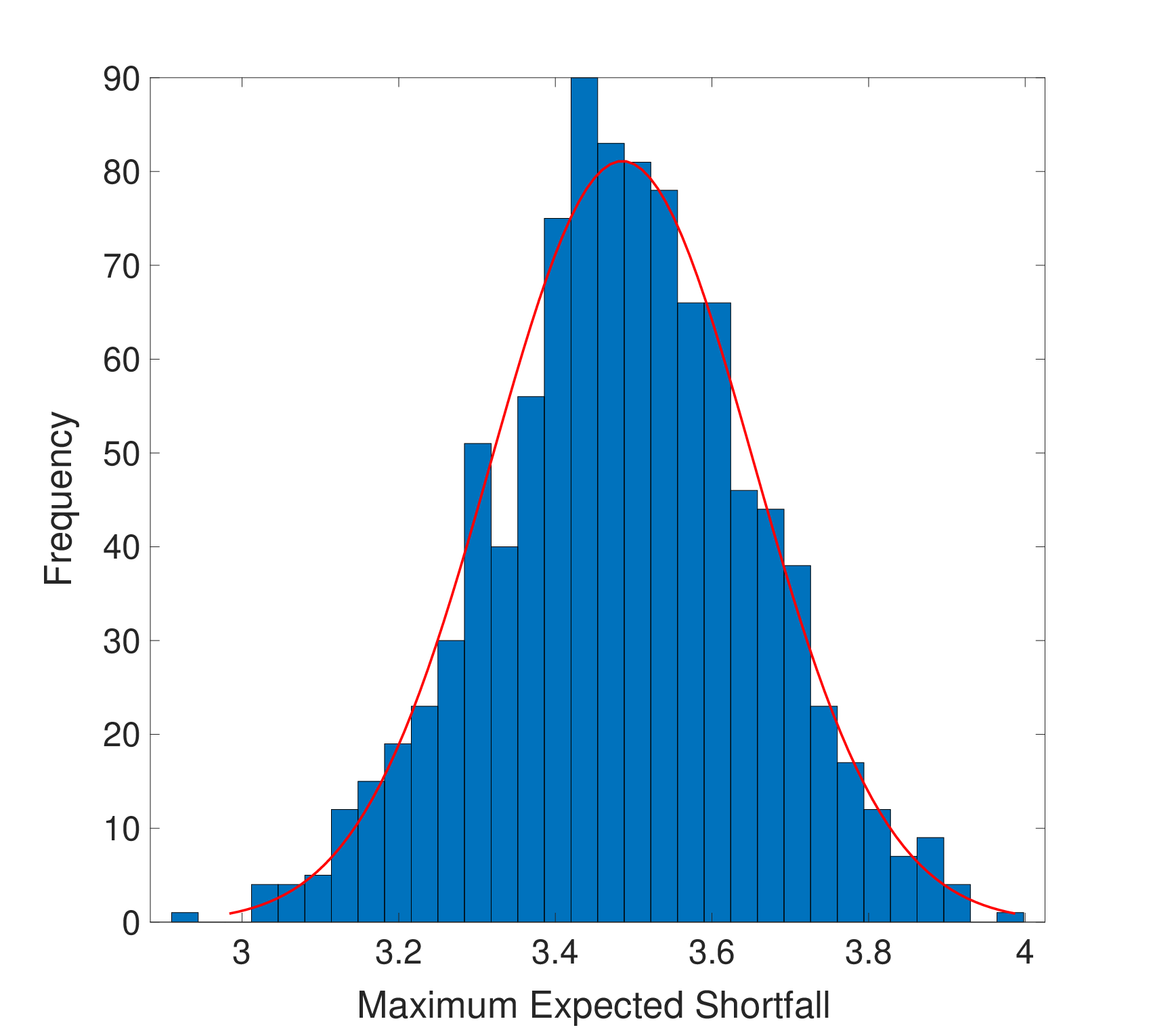
As a first example, consider the loss , with and . The optimal coupling is , so that is Gaussian with mean 0 and standard deviation 2. For generated random samples, the MES will again be attained by a comonotonic coupling. The ES of the sampled problem will then simply be the sum of the estimated ESs from the samples from and . Known results on the estimation of risk measures (e.g., Manistre and Hancock 2005) imply that the limit distribution will be Gaussian. Figures 1a and 1b show the results of a computational experiment, in which a sample of size 200 was generated from , a sample of size 400 was simulated from , and the MES with was estimated by solving the linear program (15). This experiment was repeated 1000 times, and the histogram of the optimal values is presented in Figure 1a. The q-q plot against a fitted normal is displayed in Figure 1b. An Anderson-Darling test of normality was not able to reject the null hypothesis of a normal distribution for the simulated optimal values at the 95% confidence level.

Example 2 (Counterparty Credit Risk).
A loss function related to counterparty credit risk (see, e.g. Memartoluie et al. 2017) would be the following:
where is the standard normal cumulative distribution function. This gives the systematic credit losses in the Vasicek model, with systematic credit factor , for a portfolio consisting of two counterparties with probabilities of default and , systematic credit factor loadings and , and counterparty portfolio values and , where we assume for simplicity that
We simulated 500 values from each of and , and then solved problem (15) for the MES at , with the model parameters , , , , , . The histogram of 1000 realized optimal values is given in Figure 2a. The distribution does not appear to be normally distributed, and indeed we provide on the figure the fitted Generalized Extreme Value (GEV) distribution, and the corresponding qq-plot in Figure 2b. It should be noted that Theorem 3 does not apply, as we are simulated from continuous random variables.77 7 Nonetheless, there is some evidence that similar properties to those identified in the Theorem may be at play here. Inspecting the optimal dual variables in the simulated linear programs showed them often to be very different in different simulation runs, which may be evidence that the optimal dual solution of the limiting problem is not unique.


7 Conclusions and Future Directions
In this paper, we study the problem of bounding a spectral risk measure applied to a loss function when the marginal distributions of the factors are known, but their joint distribution is unknown. Basic properties of the optimization problem, as well as an analogue of the Kantorovich (strong) duality from optimal transport were derived. Further, we studied continuity properties of the objective value and set of maximizers with respect to perturbation of the marginal constraints, as well as the distribution of the optimal value when the factor marginal distributions are simulated from finite probability spaces.
There are a number of possible directions for continuation of the research in this paper, including the following:
- •
Bounds based solely on knowledge of marginal distributions are known to often produce extreme values in practice. Following the work of Glasserman and Yang 2018 on CVA, functions that penalized a measure of “unfitness” of could be introduced into the primal problem.
- •
The distribution and convergence properties of the optimal value function could be investigated under more general assumptions on the underlying spaces , than the rather restrictive assumptions imposed in Section 6. Given that this problem is not entirely resolved even in the case of optimal transport, this is likely to be challenging.
- •
Numerical methods for the resulting optimization problems could be studied. In the work Memartoluie et al. 2017 that motivated this study, the market and credit factors were simulated independently from their marginal distributions, as in Section 6. Is there a better way to simulate the factors from their marginal distributions to yield more efficient numerical procedures? Can importance sampling algorithms be developed to yield better estimates of risk bounds given finite computational resources? Can the special structure of the optimization problem be exploited to yield more efficient numerical algorithms, given that the linear programs that must be solved can become very large?
We leave these important questions for future research.
References
- Ajtai et al. [1984] M. Ajtai, J. Komlós, and G. Tusnády. On optimal matchings. Combinatorica, 4(4):259–264, 1984.
- Ambrosio et al. [2019] L. Ambrosio, F. Stra, and D. Trevisan. A PDE approach to a 2-dimensional matching problem. Probability Theory and Related Fields, 173:433–477, 2019.
- Artzner et al. [1999] P. Artzner, F. Delbaen, J.-M. Eber, and D. Heath. Coherent measures of risk. Mathematical Finance, 9:203–228, 1999.
- Basel Committee on Banking Supervision [2019] Basel Committee on Banking Supervision. Minimum capital requirements for market risk. Technical report, Bank for International Settlements, 2019. Available at www.bis.org.
- Beiglböck et al. [2013] M. Beiglböck, P. Henry-Labordère, and F. Penkner. Model-independent bounds for option prices: A mass transport approach. Finance and Stochastics, 17:477–501, 2013.
- Bergin [1999] J. Bergin. On the continuity of correspondences on sets of measures with restricted marginals. Economic Theory, 13:471–481, 1999.
- Beutner and Zähle [2010] E. Beutner and H. Zähle. A modified functional delta method and its application to the estimation of risk functionals. Journal of Multivariate Analysis, 101(10):2452–2463, 2010.
- Bobkov and Ledoux [2019] S. Bobkov and M. Ledoux. One-Dimensional Empirical Measures, Order Statistics, and Kantorovich Transport Distances. Number 1259 in Memoirs of the American Mathematical Society. American Mathematical Society, 2019.
- del Barrio and Loubes [2019] E. del Barrio and J.-M. Loubes. Central limit theorems for empirical transportation cost in general dimension. Annals of Probability, 47(2):926–951, 2019.
- del Barrio et al. [1999] E. del Barrio, E. Giné, and C. Matrán. Central limit theorems for the Wasserstein distance between the empirical and the true distributions. Annals of Probability, 27(2):1009–1071, 1999.
- del Barrio et al. [2019] E. del Barrio, P. Gordaliza, and J.-M. Loubes. A central limit theorem for transportation cost on the real line with application to fairness assessment in machine learning. Information and Inference, 8(4):817–849, 2019.
- Delbaen [2002] F. Delbaen. Coherent risk measures on general probability spaces. In K. Sandmann and P. Schönbucher, editors, Advances in Finance and Stochastics. Essays in Honour of Dieter Sondermann, pages 1–37. Springer, 2002.
- Delomestny and Krätschmer [2012] D. Delomestny and V. Krätschmer. Central limit theorems for law-invariant coherent risk measures. Journal of Applied Probability, 49(1):1–21, 2012.
- Dudley [2002] R.M. Dudley. Real Analysis and Probability. Cambridge University Press, Cambridge, second edition, 2002.
- Embrechts et al. [2015] P. Embrechts, B. Wang, and R. Wang. Aggregation-robustness and model uncertainty of regulatory risk measures. Finance and Stochastics, 19(4):763–790, 2015.
- Ethier and Kurtz [1986] S.N. Ethier and T.G. Kurtz. Markov Processes: Characterization and Convergence. John Wiley & Sons, New York, 1986.
- Föllmer and Schied [2016] H. Föllmer and A. Schied. Stochastic Finance: An Introduction in Discrete Time. de Gruyter, Berlin, fourth edition, 2016.
- Fournier and Guillin [2015] N. Fournier and A. Guillin. On the rate of convergence in Wasserstein distance of the empirical measure. Probability Theory and Related Fields, 162:702–738, 2015.
- Galichon [2016] A. Galichon. Optimal Transport Methods in Economics. Princeton University Press, Princeton, 2016.
- Galichon [2017] A. Galichon. A survey of some recent applications of optimal transport methods to econometrics. The Econometrics Journal, 20(2):C1–C11, 2017.
- Galichon et al. [2014] A. Galichon, P. Henry-Labordère, and N. Touzi. A stochastic control approach to no-arbitrage bounds given marginals, with an application to lookback options. The Annals of Applied Probability, 24(1):312–336, 2014.
- Garcia-Cespedes et al. [2010] J.C. Garcia-Cespedes, J.A. de Juan Herrero, D. Rosen, and D. Saunders. Effective modelling of wrong-way risk, CCR capital and alpha in Basel II. Journal of Risk Model Validation, 4(1):71–98, 2010.
- Ghossoub and Saunders [2020] M. Ghossoub and D. Saunders. On the continuity of the feasible set mapping in optimal transport. Working Paper, 2020.
- Glasserman and Yang [2018] P. Glasserman and L. Yang. Bounding wrong-way risk in CVA calculation. Mathematical Finance, 28:268–305, 2018.
- Henry-Labordère [2017] P. Henry-Labordère. Model-Free Hedging. CRC Press, Boca Raton, 2017.
- Klatt et al. [2019] M. Klatt, C. Tameling, and A. Munk. Empirical regularized optimal transport: Statistical theory and applications. Available at arxiv.org, 2019.
- Klatt et al. [2020] Marcel Klatt, Axel Munk, and Yoav Zemel. Limit laws for empirical optimal solutions in stochastic linear programs, 2020.
- Kolmogorov and Fomin [1975] A.N. Kolmogorov and S.V. Fomin. Introductory Real Analysis. Dover, New York, 1975.
- Krätschmer et al. [2012] V. Krätschmer, A. Schied, and H. Zähle. Qualitative and infinitesimal robustness of tail-dependent statistical functionals. Journal of Multivariate Analysis, 103:35–47, 2012.
- Krätschmer et al. [2014] V. Krätschmer, A. Schied, and H. Zähle. Comparative and qualitative robustness for law-invariant risk measures. Finance and Stochastics, 18:271–295, 2014.
- Krätschmer et al. [2015] V. Krätschmer, A. Schied, and H. Zähle. Quasi-Hadamard differentiability of general risk functionals and its application. Statistics & Risk Modeling, 32(1):25–47, 2015.
- Kusuoka [2001] S. Kusuoka. On law invariant coherent risk measures. Advances in Mathematical Economics, 3:83–95, 2001.
- Ledoux [2017] M. Ledoux. On optimal matching of gaussian samples. Zap. Nauchn. Sem. S.-Peterburg. Otdel. Mat. Inst. Steklov. (POMI), 457:226–264, 2017.
- Ledoux [2018] M. Ledoux. On optimal matching of gaussian samples II. Available at https://perso.math.univ-toulouse.fr/ledoux/publications-3/, 2018.
- Ledoux and Zhu [2019] M. Ledoux and J. Zhu. On optimal matching of gaussian samples III. Available at https://perso.math.univ-toulouse.fr/ledoux/publications-3/, 2019.
- Lucchetti [2006] R. Lucchetti. Convexity and Well-Posed Problems. Canadian Mathematical Society, 2006.
- Makarov [1981] G. Makarov. Estimates for the distribution function of a sum of two random variables when the marginal distributions are fixed. Theory of Probability and its Applications, 26:803–806, 1981.
- Manistre and Hancock [2005] B.J. Manistre and G.H. Hancock. Variance of the CTE estimator. North American Actuarial Journal, 9(2), 2005.
- McNeil et al. [2015] A.J. McNeil, R. Frey, and P. Embrechts. Quantitative Risk Management. Princeton University Press, Princeton, second edition, 2015.
- Memartoluie [2017] A. Memartoluie. Computational Methods in Finance Related to Distributions with Known Marginals. PhD thesis, University of Waterloo, 2017.
- Memartoluie et al. [2017] A. Memartoluie, D. Saunders, and T. Wirjanto. Wrong-way risk bounds in counterparty credit risk management. Journal of Risk Management in Financial Institutions, 10(2):150–163, 2017.
- Ok [2007] E. Ok. Real Analysis with Economic Applications. Princeton University Press, 2007.
- Pflug and Wozabal [2010] G. Pflug and N. Wozabal. Asymptotic distribution of law-invariant risk functions. Finance and Stochastics, 14:397–418, 2010.
- Pichler [2010] A. Pichler. Distance of Probability Measures and Respective Continuity Properties of Acceptability Functionals. PhD thesis, Universität Wien, 2010.
- Pichler [2013a] A. Pichler. The natural Banach space for version independent risk measures. Insurance: Mathematics and Economics, 53(2):405–415, 2013a.
- Pichler [2013b] A. Pichler. Evaluations of risk measures for different probability measures. SIAM Journal on Optimization, 23(1):530–551, 2013b.
- Rachev and Rüschendorf [1998] S.T. Rachev and L. Rüschendorf. Mass Transportation Problems. Springer, New York, 1998.
- Rockafellar and Wets [2009] R.T. Rockafellar and R.J-B. Wets. Variational Analysis. Springer, New York, 2009.
- Rockefellar and Uryasev [2000] R.T. Rockefellar and S. Uryasev. Optimization of conditional value-at-risk. Journal of Risk, 2(3):21–41, 2000.
- Rosen and Saunders [2010] D. Rosen and D. Saunders. Computing and stress testing counterparty credit risk capital. In E. Canabarro, editor, Counterparty Credit Risk, pages 245–292. RiskBooks, 2010.
- Rosen and Saunders [2012] D. Rosen and D. Saunders. CVA the wrong way. Journal of Risk Management in Financial Institutions, 5(3):252–272, 2012.
- Rüschendorf [1982] L. Rüschendorf. Random variables with maximum sums. Advances in Applied Probability, 14:623–632, 1982.
- Rüschendorf [2013] L. Rüschendorf. Mathematical Risk Analysis. Springer, Berlin, 2013.
- Shapiro [2013] A. Shapiro. On Kusuoka representation of law invariant risk measures. Mathematics of Operations Research, 38(1):142–152, 2013.
- Sommerfeld and Munk [2018] M. Sommerfeld and A. Munk. Inference for empirical Wasserstein distances on finite spaces. Journal of the Royal Statistical Society: Series B, 80(1):219–238, 2018.
- Talagrand [2014] M. Talagrand. Upper and Lower Bounds for Stochastic Processes. Springer, Berlin, 2014.
- Talagrand [2018] M. Talagrand. Scaling and non-standard matching theorems. Comptes Rendus Acad. Sciences Paris, Mathématique, 356:692–695, 2018.
- Tameling et al. [2017] C. Tameling, M. Sommerfeld, and A. Munk. Empirical optimal transport on countable metric spaces: Distributional limits and statistical applications. Available at arxiv.org, 2017.
- van der Vaart [1998] A.W. van der Vaart. Asymptotic Statistics. Cambridge University Press, 1998.
- Villani [2003] C. Villani. Topics in Optimal Transportation. American Mathematical Society, Providence, 2003.
- Villani [2008] C. Villani. Optimal Transport, Old and New. Springer, Berlin, 2008.
- Zălinescu [2002] C. Zălinescu. Convex Analysis in General Vector Spaces. World Scientific, 2002.