Modeling social media contagion using Hawkes processesThanks: This work is partially supported by Polish National Science Centre Grant No. 2016/23/B/HS4/00566, 2017-2020

Nearly every day one can hear about situations in which a single incident causes a series of similar events in a short time interval. Multiple aftershocks or increased seismic activity not only in the place of the earthquake occurrence, but also in surrounding locations, are one of the most common examples. Another one can be a crash on the US stock market influencing the rest of the world’s financial markets. This kind of events are often called a cascade effect. This type of phenomenon can be observed in social media as well when repeated activation is allowed. In this paper we focus on retweet cascades where users allow to re-share content posted by other people with public accounts.

The first main goal of this paper is to model this type of behaviour by a Hawkes process. This process was proposed by Hawkes [14] to describe the dynamics changing in time in which every event causes an increase in the probability of next events occurring. Although the term ”Hawkes process” has been used in scientific literature since the early 1970s, the model gained popularity only in the last decade. Its popularity is gained by its clustering property.

The second goal of this paper is to construct calibration method of the Hawkes process based on identifying its infinitesimal generator. Then we show how to apply it in modelling retweet cascades. This work combines elements of the probability theory, statistics, the theory of stochastic processes and computer simulations.

Modelling using Hawkes have been widely used in many areas. The moments method in this context was described in [5]. Similar considerations have been performed in the context queues driven by Hawkes processes in [8], where generator method has been also applied. This method can be also applied for other Markov process whose moments are easy to compute by exploiting the structure of a new sequence of nested matrices called Matryoshkhan matrices; see [9] for details. One can work with generalization of the Hawkes process as well called the ephemerally self-exciting process; see [10]. The connection of the Hawkes process with social media has not been yet understood well though, in our opinion. The first attempt can be found in [19]. The contagion dynamics in social media have been observed and confirmed in many papers and in many contexts, see e.g. [2, 3, 4, 13, 17, 21, 18] and references therein.

The paper is organized as follows. In Section 2 we present main theoretical facts and we give there our first main result concerning generator of the Hawkes process. In next section we present estimation method of the Hawkes processes parameters. In Section 4 we show how to model retweet cascades using previous analysis. Finally, Section 5 concludes this paper. All proofs are shifted to Appendix to gain the readability of main message of this work.

The (Markov) Hawkes process $N_{t}$ was first time defined by Alan G. Hawkes in 1971 in his seminal work [14] as a counting process which intensity

at the moment $t$ depends on its natural history $\mathcal{F}_{t}$ till that moment, that is, it solves the following stochastic differential equation

where $\beta>\alpha>0$ and $\lambda_{\infty}>0$ is a fixed constant called the base intensity. Note that

where $\{T_{k}\}_{k=1,2,\ldots}$ are consecutive moments of jumps of $N_{t}$. Moreover, we have that $N_{0}=0$, $\mathbb{P}(N_{t+h}-N_{t}=0\,|\,\mathcal{F}_{t})=1-\lambda_{t}\,h+o(h)$, $\mathbb{P}(N_{t+h}-N_{t}=1\,|\,\mathcal{F}_{t})=\lambda_{t}\,h+o(h)$ and $\mathbb{P}(N_{t+h}-N_{t}>1\,|\,\mathcal{F}_{t})=o(h),$ where $o(h)$ denotes quantity tending to zero as $h$ tends to zero. Therefore, each jump of the process $N_{t}$ brings an increase in its intensity function by value $\alpha$ which increases in turn the likelihood of another jump. This is why this process is called a self-exciting process. Then the intensity function decays exponentially to the base level $\lambda_{\infty}$ at a rate given by the factor $\beta$. The condition $\beta>\alpha$ is necessary to avoid the so-called process explosion.

The Hawkes process simulation algorithm was proposed by Dassios and Zhao [7]. The algoritm presented in their work can be implemented in the R programming language (see Algoritm 1 in Appndix) and one of its exemplary outcomes is shown in Figure 1.

The clustering effect was not directly visible in the definitions and formulas cited so far, although it is a distinctive feature of the Hawkes process. For this reason, we recall an alternative equivalent definition of this process which is based on the Poisson process construction with clustering, where clusters are formed according to a recursive branching structure. More formally, Hawkes process with the exponentially decaying intensity is a Poisson cluster process. The cluster centers of $C$ are the particular points called immigrants, the rest of the points are called offspring. The Hawkes process can be constructed as follows:

1. (a)

   the immigrants are coming at moments $\widetilde{T}_{m}$ according to inhomogeneous Poisson process with rate $\lambda_{\infty}+(\lambda_{0}-\lambda_{\infty})\,e^{-\beta t}$, $t\geq 0$;

2. (b)

   each immigrant who arrived at $\widetilde{T}_{m}$ generates one cluster $C_{m}$, and all these clusters are independent of each other;

3. (c)

   each cluster $C_{m}$ is a random set formed by points of generations of order $n=0,1,\ldots$ with the following branching structure:

   • •

     the immigrant is said to be of generation 0;

   • •

     recursively, given generations $0,1,\ldots,n$ in $C_{m}$, each $\widetilde{T}_{j}\in C_{m}$ of generation $n$ generates a Poisson process of offspring of generation $n+1$ on $(\widetilde{T}_{j},\infty)$ with intensity $\alpha e^{-\beta(t-\widetilde{T}_{j})},\,t>\widetilde{T}_{j}$, independent of generations $0,1,\ldots,n$;

4. (d)

   $C$ consists of the union of all clusters, i.e. $C=\bigcup_{m=1,2,\ldots}C_{m}$ (see [7]).

This means that first the generation of the so-called ”immigrants” is generated. These are jump moments of the non-stationary Poisson process with the intensity function equal to the deterministic part of the expression in (2). For each of them, the Poisson process is generated again with the intensity specified in the definition and with a shift in time, i.e. for $t>T_{j}$. These points are projected onto the Hawkes process timeline and treated as its jump moments. This algorithm is repeated for each of the generations. The simulation scheme for the first two generations is presented in Figure 2.

Successive generation points appear with exponentially decaying intensity, so that most of them, when projected onto the same timeline, gather near the parent. This is an obvious reason for the creation of the clusters we observe.

The first aim of this paper is to construct a new method of calibration of the Hawkes process $N_{t}$. To do so we will find its (infinitesimal) generator.

From [11] we know that the two-dimensional process $X_{t}=(\lambda_{t},\,N_{t})$ is a Markov process on $D=\mathbb{R}_{+}\times\mathbb{N}\cup\{0\}$. For a sufficiently regular function $k:D\rightarrow\mathbb{R}$ we define the generator of $X_{t}$ as the following limit

with $\mathbb{E}_{t}^{x}[\quad\cdot\quad]=\mathbb{E}^{x}[\quad\cdot\quad|\mathcal{F}_{t}\quad{\rm and}\quad X_{t}=x]$. We will call the family of functions, for which the limit in the definition of the generator makes sense, the domain of the generator $\mathcal{A}$ and denote by $\mathcal{D}(\mathcal{A})$. From Dynkin theorem we know that $M_{t}=k(X_{t})-k(X_{0})-\int_{0}^{t}\mathcal{A}k(X_{s})\operatorname{d}\!s,\,t\geq 0$ is a martingale with respect to the filtration $\mathcal{F}_{t}$. Thus from Optional Stopping Theorem we can conclude that

This will be used later in a statistical procedure. Our first main result identifies the generator $\mathcal{A}$.

The proof of this theorem will be given in Appendix.

We will now present the moment method of estimating all parameters of Hawkes process, that is, estimating $\lambda_{\infty}$, $\lambda_{0}$, $\beta$ and $\alpha$. We observe our Hawkes process within finite time, that is between $t$ and $t+\Delta$, where $\Delta>0$. We will identify above parameters by finding moments $\mathbb{E}\big[N_{t+\Delta}-N_{t}\big]^{k}$.

The main idea is based on using formula (3) together with Theorem 1. Taking $k(X_{t})=k(\lambda_{t},N_{t})=N_{t}^{l}\,(l\in\mathbb{N})$ we get

which is equivalent to

Hence

Similarly, by taking $k(X_{t})=k(\lambda_{t},N_{t})=\lambda_{t}^{m}$ and $k(X_{t})=k(\lambda_{t},N_{t})=\lambda_{t}^{m}N_{t}^{l}$, we derive

and

These identities will produce equations for the mixed moments $\mathbb{E}[\lambda_{t}^{m}\,N_{t}^{l}]$ as functions of $t$ that could be solved explicitly. These moments allow to find $\mathbb{E}\big[N_{t+\Delta}-N_{t}\big]^{k}$ for $k=1,2,3$. We start first from finding the first moment given in the following theorem. We denote

The proof of this theorem will be given in Appendix. The expression given in (9) depends on the initial intensity $\lambda_{0}$, but based on the equation (2) we can conclude that for increasingly larger $t$ the influence of this constant on the value of the process intensity function is negligible. Therefore following [1] we focus on the long-run behavior of the process from now on. We need then two more moments to find $3$ parameters of Hawkes process, namely, $\lambda_{\infty}$, $\beta$ and $\alpha$.

Later, in Appendix we will prove another two key facts given in next theorem.

Having moments $\mathbb{E}\big[N_{t+\Delta}-N_{t}\big]^{k}$ for $k=1,2,3$ identified we can produce moment estimators $\hat{\alpha}$, $\hat{\beta}$ and $\hat{\lambda}_{\infty}$ of $\alpha$, $\beta$ and $\lambda_{\infty}$, respectively, by solving the system of equations:

where $\mathbb{M}_{i}$ is the arithmetic mean of the expressions of the form $(N_{t_{j}+\Delta}-N_{t_{j}})^{i}$, $t_{j}$ are the points in time mutually distant from each other by $\Delta$ and $N_{t_{j}}$ are observed values of our process.

To analyze how good is this estimation method we generated Hawkes process’ trajectories using the algorithm mentioned in Section 2 (see: Appendix, Algorithm 1). We set the parameters to $\alpha=0.2$, $\beta=1$ and $\lambda_{\infty}=1$. Due to the fact that the derived formulas are true for large $t$, it was decided to take into account the values of $N_{t+\Delta}-N_{t}$ for $t$ between $3000$ and $10000$. Besides it, we took $\Delta=0.5$. The system of equation (13) is non-linear, and the function nleqslv built in one of the R programming language packages was used to solve it. As many other numerical methods, it was necessary to specify the initial values for the algorithm which were set to $\alpha=0.5$, $\beta=1.5$ and $\lambda_{\infty}=2$.

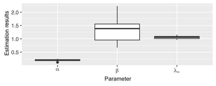
The results of the estimation are given in Table 1. Notice that the estimator of the parameter $\lambda_{\infty}$ fares surprisingly well. Based on twenty simulations, we obtain an average result of $1.056\pm 0.054$, which is very close to the real value $\lambda_{\infty}=1$. For the estimators of $\alpha$ and $\beta$ , we get average values of $0.198\pm 0.031$ (which is also a very good result) and $1.350\pm 0.474$, respectively. Figure 3 shows that despite the identical values of the actual $\beta$ and $\lambda_{\infty}$, as well as the fact that the initial $\beta$ value given for the algorithm was closer to the real value than it was for $\lambda_{\infty}$, the $\hat{\beta}$ estimator is much worse than $\hat{\lambda}_{\infty}$.

Our last and main goal is to show that Hawkes process can indeed model clustering behaviour in social media. We decided to analyze one of the most popular websites, Twitter, which allows users to re-share content posted by other people with public accounts. This is called a retweet. With each retweet, the original post reaches a new audience who can also pass it on to their followers. If we marked on the axis the time points at which users retweeted the original tweet, we would most likely observe their clustering.

One of the most popular accounts on Polish Twitter is the account of the president of Poland, Andrzej Duda (@AndrzejDuda). Due to its popularity, it may prove to be an interesting source of data for analysis and modeling using the Hawkes process. This account is public, so each tweet can be retweeted by other Twitter users. The post presented in Fig. 4 was retweeted exactly $556$ times at the time of analysis.

Unfortunately, due to Twitter API limitations and user privacy settings, it is not possible to obtain accurate data. Some users block access to their tweets for people who do not follow them, so we cannot obtain information about the time when they retweeted the post we were analyzing. Using the Python tweepy module, which enables easy use of Twitter API, it was possible to obtain information on $448$ retweets, which is about 80% of the total. Their distribution over time is shown in the graph in Figure 5, where the horizontal axis represents the time since the original post was published.

There are clear changes in dynamics here. The total number of retweets increases sharply in the first few minutes after publishing the post. Then the speed of growth slows down slightly to rise again after about $6$ hours (perhaps the post was retweeted by another popular account). Further, the process stabilizes, the increase in the number of retweets is negligible. In [19], a similar analysis was performed, in which the author of the post was an account with over $12,000$ followers, and the time horizon was set to $600$ seconds. Since Andrzej Duda’s account has definitely more followers (over $1.1$ million), adopting a time horizon of $10$ hours seems to make sense. The time for a tweet to be retweeted by another user is made available with an accuracy of one second, but because the delta should be small, the base unit we take is minutes, so $\Delta=\frac{1}{60}\,[min]$, and the time horizon was set at $10$ hours. Figure 6 presents the analyzed data.

The numerical method of solving a system of nonlinear equations (13) requires specifying an initial point, which can be any of the domains we allow. Assuming $(\alpha,\beta,\lambda_{\infty})=(0.5,1.5,0.75)$ as the starting point, the result of the estimation is approximately $\alpha=0.772,\beta=1.133,\lambda_{\infty}=0.243$. Assuming that $\lambda_{0}$ is the same as $\lambda_{\infty}$, , the intensity graph of this process would look like in Fig. 7. Using the formula from equation we can check that with these parameters the expected value of the process at time $t=600$ (10 hours) is $\mathbb{E}N_{600}=348.7265$. The actual number of retweets up to that point was $342$.

To validate the estimation results, twenty possible Hawkes process trajectories were generated for the parameter set $\alpha=0.772,\beta=1.133,\lambda_{\infty}=\lambda_{0}=0.243$. These trajectories, marked with gray lines, were compared in Fig. 8 with the actual number of retweets in time (marked with a red line). We observe a significant deviation from the norm at the beginning of the process, the number of retweets in the first minutes increases too rapidly. It only starts to resemble the generated trajectories after about $400$ minutes. This may suggest that a different model would be necessary to be able to describe the dynamics of the spread of content posted by popular accounts in the early stage of the process.

In this paper, using the generator theory, we describe moments method of estimation of the parameters of Hawkes process. We apply it to show that in social media quite often the clustering phenomenon might appear. As an example we analyze retweet cascades. The results based on the twenty generated trajectories turned out to be surprisingly good, however, showing a relatively large variance of the $\beta$ parameter estimate compared to the other two. It would be good to look for other possible applications of Hawkes process in social media and present paper can seen as the first step toward deeper understanding the contagion dynamics there.

References

• [1] Y. Ait-Sahalia, J. Cacho-Diaz, and R. Laeven. Modeling financial contagion using mutually exciting jump processes. National Bureau of Economic Research, Inc, NBER Working Papers, 117, 2010. doi: 10.2139/ssrn.1363882.
• [2] S. Aral, L. Muchnik, and A. Sundararajan. Distinguishing influence-based contagion from homophily-driven diffusion in dynamic networks. PNAS 106 (51): 21544–21549, 2009.
• [3] S. Aral, L. Muchnik, and A. Sundararajan. Engineering social contagions: optimal network seeding in the presence of homophily. Netw. Sci. 1 (02): 125–153, 2013.
• [4] D. Centola and M. Macy. Complex contagions and the weakness of long ties. Am. J. Sociol. 113 (3): 702–734, 2007.
• [5] L. Cui, A. Hawkes, and H. Yi. An elementary derivation of moments of Hawkes processes. Adv. Appl. Prob., 52(1): 102–137, 2020.
• [6] J. Da Fonseca and R. Zaatour. Hawkes Process: Fast Calibration, Application to Trade Clustering, and Diffusive Limit. Journal of Futures Markets, 34, 2014. doi: 10.1002/fut.21644.
• [7] A. Dassios and H. Zhao. Exact simulation of Hawkes process with exponentially decaying intensity. Electronic Communications in Probability, 18:3–7, 2013. doi: 10.1214/ECP.v18-2717.
• [8] A. Daw and J. Pender. Queues Driven by Hawkes Processes. Stochastic Systems 8(3): 192–229, 2018.
• [9] A. Daw and J. Pender. Matrix Calculations for Moments of Markov Processes. https://arxiv.org/abs/1909.03320, 2019.
• [10] A. Daw and J. Pender. An Ephemerally Self-Exciting Point Process. https://arxiv.org/pdf/1811.04282.pdf, 2018.
• [11] E. Errais, K. Giesecke, and L. R. Goldberg. Affine Point Processes and Portfolio Credit Risk. SIAM Journal on Financial Mathematics, 1:642–665, 2010. doi: 10.1137/090771272.
• [12] P. Ge and R. Blumenthal. Markov processes and potential theory. ISSN. Elsevier Science, 2011. ISBN 9780080873411.
• [13] M. Gladwell. Small Change. Why the Revolution Will Not Be Tweeted. The New Yorker, 2010.
• [14] A. G. Hawkes. Spectra of some self-exciting and mutually exciting point processes. Biometrika, 58, 1971. ISSN 0006-3444. doi: 10.1093/biomet/58.1.83.
• [15] V. Kolokoltsov. Markov Processes, Semigroups and Generators. De Gruyter Studies in Mathematics. De Gruyter, 2011. ISBN 9783110250114.
• [16] P. J. Laub, T. Taimre, and P. K. Pollett. Hawkes Processes. https://arxiv.org/abs/1507.02822, 2015.
• [17] P. Piedrahita, J. Borge-Holthoefer, Y. Moreno, and A. Arenas. Modeling self-sustained activity cascades in socio-technical networks. Europhys. Lett. 104 (4): 48004, 2013.
• [18] P. Piedrahita, J. Borge-Holthoefer, Y. Moreno, and S. González-Bailón. The contagion effects of repeated activation in social networks. Social Networks 54: 326–335, 2018.
• [19] M.-A. Rizoiu, Y. Lee, S. Mishra and L. Xie. A tutorial on Hawkes processes for events in social media. 2017, https://arxiv.org/abs/1708.06401.
• [20] S. Ross. Stochastic Processes. Wiley, 1995.
• [21] D. Watts. A simple model of global cascades on random networks. PNAS 99: 5766–5771, 2002.