Two-Loop Five-Parton Leading-Colour Finite Remainders in the Spinor-Helicity FormalismPreprint: FR-PHENO-2020-017, IPPP/20/50

The original calculation in Ref. Abreu:2019odu was performed via numerical $D$-dimensional generalised unitarity in the leading-colour approximation, more precisely in the limit of large number of colours $N_{c}$ while keeping the ratio to the number of flavours $N_{f}$ fixed.

The full amplitudes $A$ are stripped of their dependence on the gauge-group factors by colour-ordering decompositions Ochirov:2019mtf; Ochirov:2016ewn in terms of color-ordered sub-amplitudes $\mathcal{A}$. Their expansion in terms of the bare QCD coupling $\alpha_{0}$ reads

where $\mathcal{A}^{(n)}$ is a $n$-loop amplitude. Each loop amplitude can be further expanded in the ratio $N_{f}/N_{c}$ as

Bare quantities are related to renormalised ones through the running of the QCD coupling $\alpha_{s}(\mu)$, whose relation to the bare coupling $\alpha_{0}$ is given by the $\beta$-function

with $S_{\epsilon}=(4\pi)^{\epsilon}e^{-\epsilon\gamma_{E}}\,$. This, in turn, leads to the renormalised amplitude

The $\epsilon$-pole dependence of an $n$-loop amplitude is determined by lower-loop amplitudes and well known universal factors Catani:1998bh; Sterman:2002qn; Becher:2009cu; Gardi:2009qi

The latter equation can be rearranged to obtain the definition of the so-called finite remainders, which contain the genuine two-loop information

These finite remainders can be expressed as sum of products of rational coefficients $r_{i}$ and special transcendental functions $h_{i}$ such as pentagon functions Gehrmann:2018yef; Chicherin:2020oor

Eq. 8 and 9 are valid term by term in the $N_{f}/N_{c}$ expansion of Eq. 3. The rational coefficients $r_{i}$ are the subject of the present study.

The finite-field reconstruction originally employed in Ref. Abreu:2019odu requires to choose a minimal set of linearly independent invariants. This minimal set was either momentum twistor parameters Hodges:2009hk, or a combination of Mandelstam variables, $s_{ij}=2P_{i}\cdot P_{j}$, and Gram determinants, $\text{tr}_{5}(ijkl)=\text{tr}(\gamma_{5}P_{i}P_{j}P_{k}P_{l})$. In the case of our input expressions the choice for the five-point amplitudes was

To uncover the simpler expressions, we relax this condition and instead consider an over-complete (in a linear sense) set of spinor variables¹¹ 1 For an introduction to the spinor-helicity notation please see Ref. Dixon:2013uaa; Maitre:2007jq., which for the current application can be taken to be

This set of variables was discovered by starting off with an even larger one containing all spinor contractions of a certain form and restricting it to those for which the rational functions under consideration actually display diverging behaviour.

The advantage of such a choice of variables is that there is now a one-to-one correspondence between variables and possible poles of the rational coefficients in complex momentum space. This relation can be exploited numerically, for instance via high-precision floating-point evaluations in singular limits

where $\alpha_{i,j}$ is the order of the pole ($\alpha_{i,j}<0$) or zero ($\alpha_{i,j}>0$) of the coefficient $r_{i}$ in the spinor variable $v_{j}$. If $\alpha_{i,j}$ is zero, then $v_{j}$ is neither a pole nor a zero of $r_{i}$.

After evaluating $r_{i}$ in all singular limits of Eq. 12, we obtain the least common denominator ($\mathcal{LCD}$) representation of the rational function $r_{i}$

where the quotient $\mathcal{N_{LCD}}/\mathcal{N}$ is given by the product of common factors in the numerator $\{v_{j}:\alpha_{i,j}>0\}$ or $1$ if no common factor was found. In general, $\mathcal{N}$ is guaranteed to be free from denominator factors, assuming $\vec{v}$ contains all possible poles of $r_{i}$.

Note that in some cases such as the first example given in the Appendix (23/24) the task of determining the coefficient $r_{i}$ is rendered entirely trivial by this procedure, as the product of the $v^{\alpha_{i,j}}_{j}$ factors yields the full answer up to an easily obtained constant pre-factor. More generally, the numerator $\mathcal{N}$ is a polynomial in spinor variables of Eq. 11 whose complexity depends on its mass dimension and its phase weights (see Sec. 2.3 of Ref. DeLaurentis:2019phz). The coefficients of this polynomial can be fixed by linear solving.

Let us consider the second example given in the Appendix (25/26), Eq. 13 reads²² 2 This coefficient is for $\mathcal{R}^{(2)[N_{f}^{1}]}_{g^{-}g^{+}g^{-}g^{+}g^{+}}$.

where $\mathcal{N}$ has mass dimension $14$ and phase weights $[-4,-4,-4,0,-4]$. In this case, the corresponding ansatz, i.e. a set of products of spinor brackets which spans $\mathcal{N}$, only has 160 entries. However, note that this is a fairly easy example. In general, as the number of factors in $\mathcal{D_{LCD}}$ increases, so does the size of the system corresponding to $\mathcal{N}$, and in some cases it can exceed $100\,000$ entries.

In order to simplify the reconstruction, we need to go one step further and perform a partial-fraction decomposition before actually attempting the numerator reconstruction. Such a decomposition will also better represent the pole structure of the coefficients. Thus, let us write the coefficients in the following form

This decomposition is of course not unique. If we denote by $\big[\mathcal{N}\big]$ the size of the ansatz for the expression $\mathcal{N}$, the aim is to have $\sum_{k}\big[\mathcal{N}_{k}\big]\ll\big[\mathcal{N}\big]$. This is generally achieved by picking the $\beta^{k}_{i,j}$ as large as possible.

In order to obtain insights into the structure of possible partial-fraction decomposition, we study the behaviour of $r_{i}$ in all doubly singular limits

By comparing $\alpha_{i,(j_{1},j_{2})}$ to $\alpha_{i,j_{1}}+\alpha_{i,j_{2}}$ we can infer potential partial-fraction decompositions. Since in general there will exist additional factors $v_{j_{3}\neq j_{1},j_{2}}$ that will also be of order $\sim O(\epsilon)$ in this double limit, the logic to apply to extract useful information out of the table of exponents $\alpha_{i,(j_{1},j_{2})}$ can be fairly lengthy. We refer the reader to Ref. DeLaurentis:2019phz for a detailed discussion. Let us consider an example instead.

In the case we already considered (25/26), two of the doubly singular limits are

Therefore, it is logical to conjecture that if we want to reconstruct the residue of $\langle 5|1+2|5]^{3}$ we need to include in the denominator the full fourth order pole $[13]^{4}$ but $[25]$ may suffice as a simple pole. Indeed this is the case, as shown by the first fraction in 26.

This strategy appears to scale well with the size of $\mathcal{D_{LCD}}$, severely limiting $[\mathcal{N}_{k}]$ even in the most complicated cases. Furthermore, as explained in Ref. DeLaurentis:2019phz, specific numerators $\mathcal{N}_{k}$ can be isolated and reconstructed individually by generating phase-space points in limits where they are dominant. This allows to solve a few small systems instead of a single large one, and to apply the strategy iteratively by recursively subtracting reconstructed partial-fractioned terms and repeating the study of the singular limits for the remainder.

We compare the complexity of our expressions with the original input expressions from Ref. Abreu:2019odu which were simplified by means of Leinartas partial fractioning leinartas1978factorization; raichev2012leinartass. As a measure of complexity we use the leaf count.

Figure 1 shows the ratio of the leaf counts for all 740 coefficients. This comparison is between the raw output of the spinor reconstruction to the Leinartas simplified version of the Mandelstam expressions. The vast majority of the coefficients is simplified in the spinor version, in some cases by more than one order of magnitude. Overall, the total new leaf count is about two times smaller, at $4\cdot 10^{6}$ compared to $9\cdot 10^{6}$. This is the case, despite the leaf count of most expressions is reduced by more than a factor of two, because the largest reduction occurred for coefficients of relative small size. As a result of the reduced complexity, the total speed up for the evaluation of all coefficients is also a factor of about 2, at about $1s$ instead of $2s$ on Mathematica.

For the results we present in this paper, we take as input numerical evaluations of analytical expressions previously obtained in Ref. Abreu:2019odu. In principle our method could have been applied directly to the numerical program from which the expressions we take as input were themselves obtained. Of course this would have required a significantly larger amount of computing resources. In this section we quantify how many numerical evaluations are needed by each method to recover the analytical expressions, and show that using our reconstruction technique would have required far fewer, albeit in some cases with higher numerical precision.

The number of evaluations required to perform the reconstruction of a numerator $\mathcal{N}_{k}$ is directly related to the size of the linear system which parametrises it. In particular, the relevant systems are Lorentz invariant polynomials with $[\mathcal{N}_{k}]$ linearly independent monomials. Let us perform the counting for a numerator of mass dimension $d$ and zero phase weights, since this case can be equivalently expressed in terms of spinor products or Mandelstam variables, $s_{ij}$, and Gram determinants, $\text{tr}_{5}(ijkl)$³³ 3 Note that there is only one linearly independent $\text{tr}_{5}$ at five-point.. Let $m$ be the multiplicity of the phase space, then the counting for the number of linearly independent $s_{ij}$ and $\text{tr}_{5}(ijkl)$ is simply

The size of the numerator ansatz is then bounded as follows

where the double parenthesis denotes combinations with replacement

Unfortunately, the exact counting valid at all-multiplicity is not easy to obtain due to the following identity

However, the upper bound of Eq. 19 is saturated at all multiplicities for mass dimensions $d\leq 4$, and at all mass dimensions for multiplicities $m\leq 5$, which includes case relevant for the current study.

Figure 2 shows the largest mass dimension of the numerators appearing in the rational coefficients of the various components of the two-loop five-parton finite remainders which need to be reconstructed either in terms of Mandelstam invariants via finite-field methods over a single denominator, or in terms of spinor variables via Gaussian elimination of partial-fractioned systems in specific kinematic configurations. In particular, the two largest systems to reconstruct have respectively mass dimension $d=68$ for the former case, which by Eq. 19 yields a system of size $132\,720$⁴⁴ 4 The actual number of evaluations used in Ref. Abreu:2019odu was 94,696 instead of the predicted 132,720, because of subtleties and optimisations in their reconstruction algorithm., and mass dimension $d=23$ for the latter case, which gives a system of size $2\,288$⁵⁵ 5 Note that Eq. 19 requires even mass dimensions. In this case the ansatz is technically for mass dimension 23 and phase weights [1, -1, 1, 1, 0].. Since the latter case corresponds to the largest numerator in a partial-fractioned ansatz, i.e. max($[\mathcal{N}_{k}]$), whereas the former to a single fraction expression, i.e. $[\mathcal{N_{LCD}}]$, for a fair comparison we should really sum over the size of the systems for all numerators in said ansatz, i.e. $\sum_{k}[\mathcal{N}_{k}]$. Yet, even then they only add up to about $6\,000$. Figure 3 shows in more details the largest numerator mass dimensions for the spinor expressions. Note that common numerator factors are not taken into account, since they multiply the ansatz and are not parametrised by the latter.

A couple of further elucidations are in order. Firstly, we always solve the linear systems with an in-house implementation of a partially-pivoted row-reduction algorithm on GPGPUs, which requires double precision floats.

Secondly, the largest linear systems, such as the one of size $2\,288$, are not generated in any singular limit. These phase-space points are only required to 16 digits and are clearly relevant for all coefficients, whereas the specific phase-space points for the other terms in the partial-fraction decomposition may be required with higher precision and depend on which residues need to be fitted. Therefore, the latter type may differ from one coefficient to another depending on which poles appear. However, note that the case used above, where the number of free parameters in these numerators add up to about $4\,000$, contains 20 of the 30 poles of Eq. 11. It is then reasonable to increase this number of $50\%$ to account for the remaining 10 poles. Still, this does not change the ball-park of up to $10\,000$ evaluations.

Thirdly, although most phase-space points are required with higher than double precision, they are also counted multiple times. For instance, if an ansatz takes the form $N_{1}/\langle 12\rangle^{2}+N_{2}/\langle 12\rangle$, in the sum over the number of free parameters for the numerators $N_{k}$ both $N_{1}$ and $N_{2}$ will appear, even though the same high-precision evaluations in the limit of small $\langle 12\rangle$ can be used for both coefficients. The true number of required evaluations would be max($[N_{1}]$, $[N_{2}]$) instead of $[N_{1}]$ + $[N_{2}]$. However, by performing this over-counting the estimate is closer to the number of equivalent double-precision evaluations need. In general the precision required depends linearly on how many sub-leading orders of a pole need to be resolved. In practice we used fixed precision evaluations with 300 digits and picked $\epsilon\sim 10^{-30}$ for the singular limits (Eq. 12) to avoid stability issues, but in theory $\epsilon\sim 10^{-16}$ and as few as 16 digits of precision per pole order could still allow to solve the systems with double precision. However, these type of stability considerations would need to be performed directly on the numerical code and not on already reconstructed expressions.

Overall, we find that the number of numerical evaluation required to perform the analytical reconstruction is reduced from about $100\,000$ to about $10\,000$. Considering the quoted evaluation time of 4.5 min per phase-space point in Ref. Abreu:2019odu, this could potentially make the calculation cheaper, depending on the additional cost of higher precision executions. Parity in this case would be obtained for an average floating-point evaluation $10\times$ slower than a finite-field one. The expectation is that as the complexity of the expressions increases, for instance as a consequence of an increased number of scales, the brute-force single-numerator reconstruction will eventually become more expensive.

The ultimate aim of expressions such as those considered in this paper is for them to be used for predictions of physical observables, such as differential cross-sections. This requires a phase-space integration to be carried out with Monte-Carlo algorithms. In calculations of loop amplitudes the numerical accuracy of the results has been a source of concern due to inherent instabilities of the methods or expressions used.

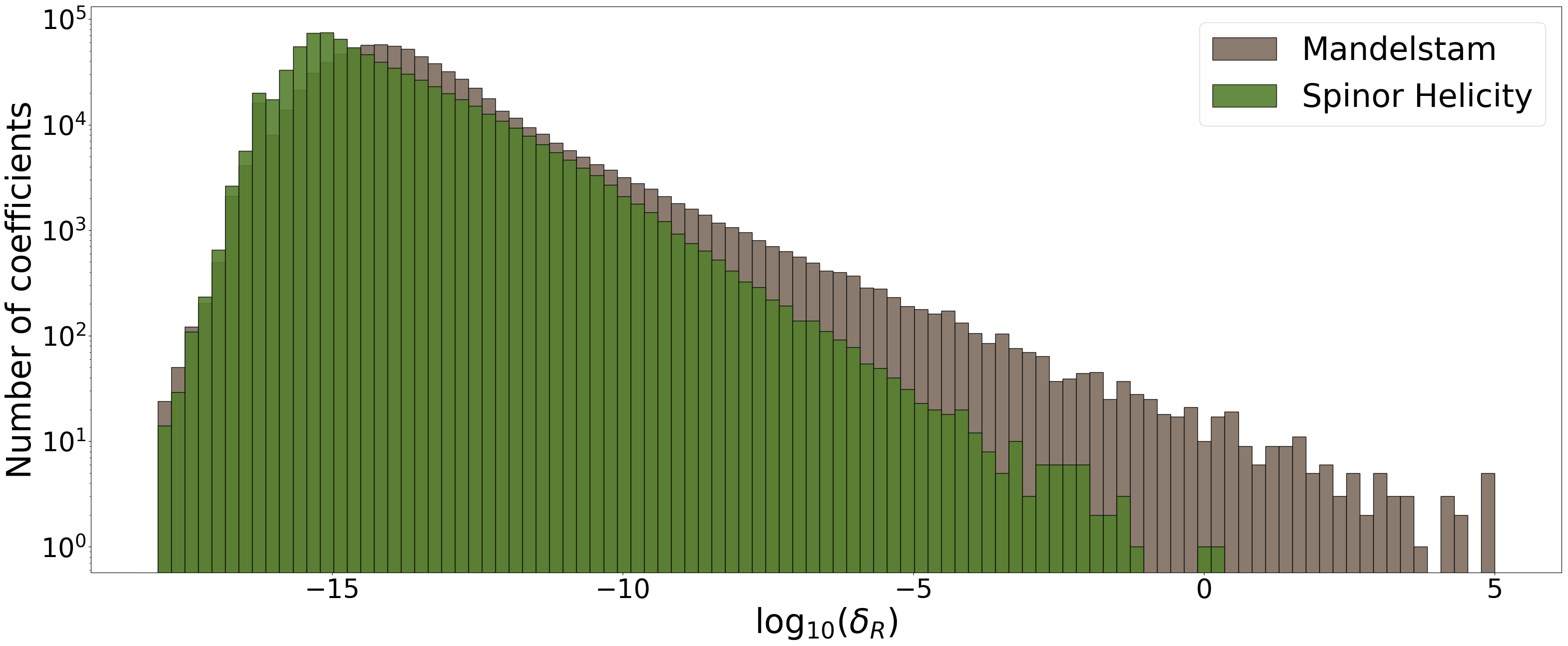
In this section, we study the double-precision floating-point numerical stability of the two-loop five-parton rational coefficients, comparing our expressions to those used as input. We do this by evaluating both sets of coefficients over $1\,000$ phase-space points. These are unweighted LO events for three-jet production at the LHC, with a center of mass energy of $14\;{\rm TeV}$, and with a jet cut of $20\;{\rm GeV}$. Care is taken that both momentum conservation and on-shell relations are satisfied to one part in $10^{16}$ for the input momenta. For each phase-space point the precision is then extended to $64$ decimal digits, the coefficients are re-evaluated and the relative error is computed as standard

We also check that in the high precision evaluation the Mandelstam and spinor expressions agree at least for 16 significant digits. This is done at all $1\,000$ phase-space points for each of the $740$ coefficients for both Mandelstam and spinor representations. The resulting two sets of $740\,000$ data points are plotted in Figure 4.

In the ideal case, all points would lie around the peaks at $-15$ on the x-axis, signifying little to no precision loss. However, we see that in practice this is not the case, with both curves displaying long tails extending towards the positive x-axis. Data points around 0 signify evaluations which ended up being $O(1)$ away from their true value: no significant digit is left and the output is pure numerical noise. It is apparent that the spinor expressions have an improved behaviour in the tail of the distribution.

Furthermore, the numerical stability is drastically increased for evaluations in soft or collinear regions of phase space. Evaluations in the collinear limit for 3-jet production at NNLO are rare, but will be important for 2-jet production at $\text{N}^{3}\text{LO}$, where these amplitudes appear as real-virtual corrections. Evaluations in the soft limit will be probed in the case of a large disparity of jet transverse momentum scales, which is relevant already for NNLO 3-jet production. For floating-point evaluations with $v_{i}\sim 10^{-x}$ and $v_{j\neq i}\sim O(1)$ one may reasonably expect to lose $x$ digits of precision per order of the $v_{i}$ pole above the true one for the given expression.

The presented expressions eliminate this type of instability by never having a pole of higher order than necessary. For instance, if we consider the first example in the Appendix, the Mandelstam expression 23 has a spurious double pole in $s_{12}$ and a spurious triple pole in $(s_{12}+s_{23}-s_{45})\sim s_{13}$, whereas the spinor expression 24 manifestly has no pole in the $s_{12}$ channel and has a triple pole in the spinor variable $[13]$, which for real kinematics corresponds to $s_{13}^{3/2}$.