An impossibility result for phylogeny reconstruction from $k$ -mer counts

Wai-Tong Louis Fan Note: Department of Mathematics, Indiana University, Bloomington. Note: Center of Mathematical Sciences and Applications, Harvard University, Cambridge. Brandon Legried Note: Department of Statistics, University of Michigan, Ann Arbor. Sebastien Roch Note: Department of Mathematics, University of Wisconsin–Madison.

August 11, 2026

Abstract

We consider phylogeny estimation under a two-state model of sequence evolution by site substitution on a tree. In the asymptotic regime where the sequence lengths tend to infinity, we show that for any fixed $k$ no statistically consistent phylogeny estimation is possible from $k$ -mer counts over the full leaf sequences alone. Formally, we establish that the joint distribution of $k$ -mer counts over the entire leaf sequences on two distinct trees have total variation distance bounded away from $1$ as the sequence length tends to infinity. Our impossibility result implies that statistical consistency requires more sophisticated use of $k$ -mer count information, such as block techniques developed in previous theoretical work.

1 Introduction

Molecular sequence comparisons are fundamental to many bioinformatics methods [Gus97, DEKM98, CP18]. In particular, the probabilistic analysis of sequences and their statistics has provided valuable insights, for instance, in comparative genomics [KA90, BC01, LHW02, RCSW09], population genetics [Tav84, PPP+06, PPR06, BAP05], and phylogenetics [Ste94, ESSW99, EKPS00, Mos04, RS17]. In this paper, we consider alignment-free phylogeny reconstruction [VA03, Hau14].

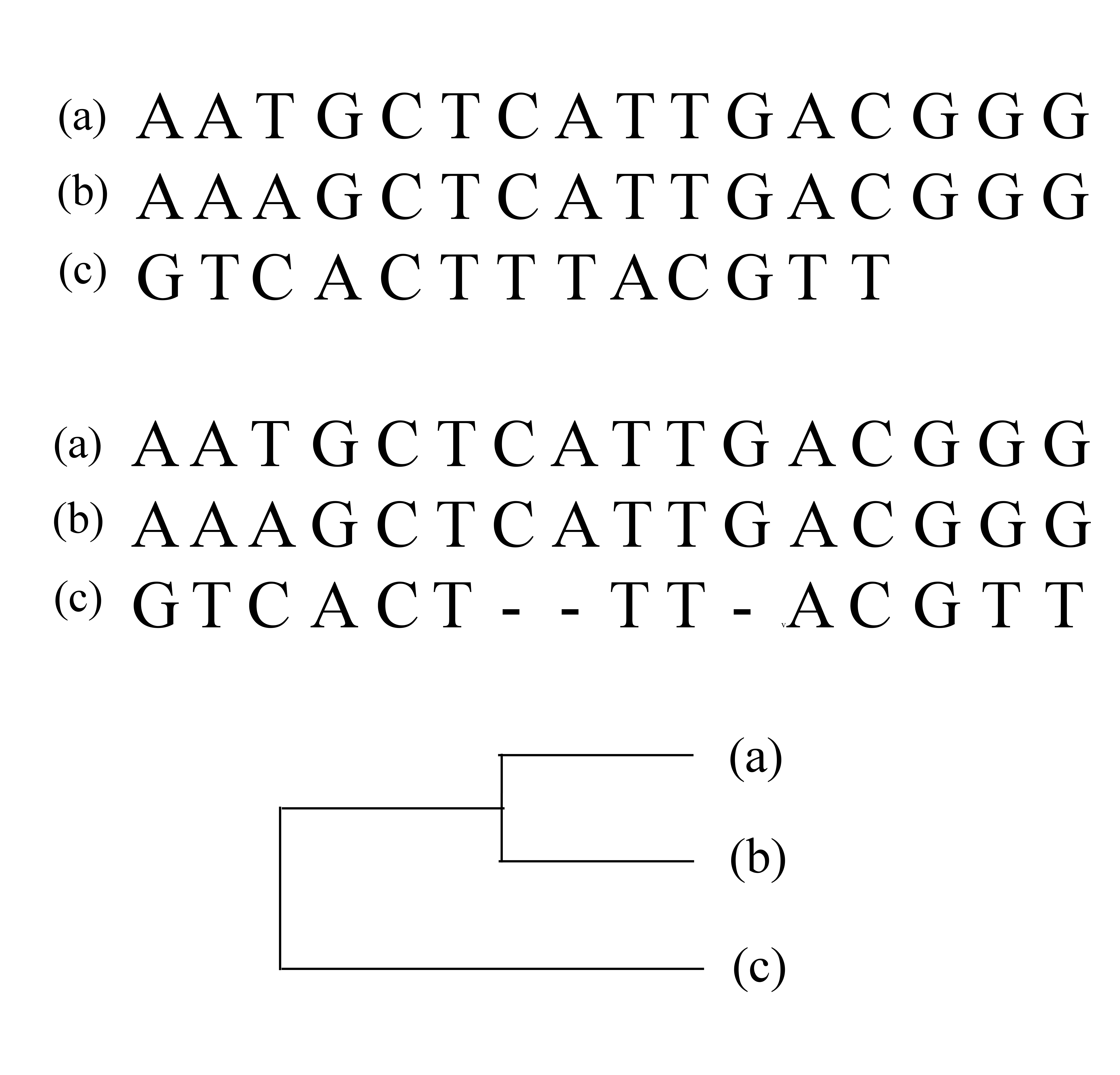
Alignment-free approaches are an important class of methods for estimating evolutionary trees that bypass the computationally hard multiple sequence alignment problem ( depicted in Figure 1) and avoid the need for a reference genome. Typically, these methods construct pairwise distances between sequences based on match lengths [UBTC06, HKP15] or $k$ -mer counts [QWH04, Hau14, FISGC15]. Here a $k$ -mer refers to a consecutive substring of length $k$ in an input sequence ( see Figure 2 for an illustration). The pairwise distance matrix obtained is then used to reconstruct the phylogenetic relationships among the sequences. A variety of standard distance-based phylogenetic methods can be used for this purpose [War17, Ste16]. Numerous popular pipelines are available that implement these alignment-free approaches [HKP15, OTM+16, LKP+18, LHTH+19], although they do not offer rigorous guarantees of accurate reconstruction.

Refer to caption — Figure 1: Standard steps in phylogeny estimation. Top: DNA sequences obtained from species (a), (b), and (c). While inherited from a common ancestor, the sequences and their lengths differ because of past mutations (including insertions and deletions). Middle: A multiple sequence alignment of the sequences, where gaps are inserted to align the columns as best as possible. Each column indicates inferred common ancestry (homology). Bottom: A rooted phylogenetic tree depicting the estimated evolutionary history of the sequences, with (a) and (b) being more closely related.

In this paper, we consider the problem of phylogeny estimation under a two-state symmetric model of sequence evolution by site substitutions on a leaf-labeled tree. In the asymptotic regime where the sequence length tends to infinity, we show that:

for any fixed $k$ , no statistically consistent phylogeny estimation is possible from the $k$ -mer counts of the entire input sequences alone.

Formally, we establish that the joint distribution of $k$ -mer counts over the entire leaf sequences on two distinct trees have total variation distance bounded away from $1$ as the sequence length tends to infinity. Put differently, these two joint distributions have a non-vanishing overlap in that asymptotic regime. Our results are information-theoretic: since the reconstruction probability of any method is only as good as the worst total variation distance (see [FR18, Lemma 3.2]), our main claim (Theorem 1) implies an impossibility result for reconstruction methods using only $k$ -mer counts across the entire sequences at the leaves. On the other hand, our results have no implications for reconstruction methods using $k$ -mer counts in more elaborate ways, e.g., through block decomposition. We come back to prior approaches of this type below in “Related work.”

To bound the total variation distance between the two distributions on well-chosen trees, our proof takes advantage of a multivariate local central limit theorem, an approach which is complicated by the probabilistic and linear dependencies of $k$ -mers.

Related work

A related impossibility result was established in our previous work [FLR20], where it was shown that no consistent distance estimation is possible from sequence lengths alone under the TKF91 model [TKF91], a more complex model of sequence evolution which also allows for insertions and deletions (indels). On the other hand, sequence lengths are significantly simpler to analyze than $k$ -mers and are not used in practice to infer phylogenies. Moreover the results in [FLR20] only apply to distance-based phylogeny estimation methods, while our current results are more general.

In a separate line of work, a computationally efficient algorithm for alignment-free phylogenetic reconstruction was developed and analyzed in [DR13]. Rigorous sequence length guarantees for high-probability reconstruction under an indel model related to the TKF91 model were established. While this method is based on $1$ -mers, it first divides up the input sequences into blocks of an appropriately chosen length and then compares the $1$ -mer counts on each block across sequences. A block in the ancestral sequence gives rise to blocks in the descendant sequences that have the same position, so the comparison does not require an alignment technique. The weak correlation between the blocks allows the use of concentration inequalities on a notion of pairwise distance proposed in [DR13]. In particular, this reconstruction method uses more information than $1$ -mer counts over the entire sequences (that is, it uses $1$ -mer counts over each separate block), so that our results do not apply to it (in the limit of zero indel rate). However no practical implementation of this $1$ -mer-based approach is available. In [DR13], accurate phylogenetic reconstruction with high probability is shown to be achievable when the sequence length is of polynomial order in the number of leaves $n$ . In a constrained regime of parameters, significantly improved bounds on the sequence length requirement were obtained in [GZ19], who used techniques related to those of [DR13] and also exploited a well-studied connection to ancestral sequence reconstruction. In other related work, it was proved in [ARS15] that the tree topology as well as mutation parameters can be identified from pairwise joint $k$ -mer count distributions under more general substitution-only models of sequence evolution using an appropriately defined notion of distance. Block techniques can then be used to derive statistical consistency results. See also [DS19] for extensions to coalescent-based models. We emphasize that the results in [DR13, ARS15, GZ19, DS19] do not contradict our main claim (Theorem 1), which excludes block decomposition.

Alignment-free sequence comparisons based on $k$ -mer counts were also studied for independent sequences with i.i.d. sites or under certain hidden Markov models of sequences [LHW02, RCSW09, WRSW10, BC01]. Because they assume independent sequences, such results are not directly relevant to phylogeny reconstruction.

Organization

The paper is organized as follows. In Section 2, we state our main results after providing the necessary background and definitions. We also sketch the main steps of the proof. The details of the proof can be found in Section 3. A few auxiliary results are in the appendix.

2 Definitions and main result

In this section, we state our result formally, after introducing the relevant concepts.

$k$ -mers.

Let $k$ be a positive integer, fixed throughout. First, we define $k$ -mers and introduce their frequencies in a binary sequence, which will serve as our main statistic.

Definition 1.

A $k$ -mer is a binary string of length $k$ , i.e., $y\in\{0,1\}^{k}$ . For a binary sequence $\sigma=(\sigma_{i})_{i=1}^{m}$ of length $m$ , we let $f_{\sigma}(y)\in\mathbb{Z}_{+}$ be the number of times $y$ appears in $\sigma$ as a consecutive substring, where $\mathbb{Z}_{+}$ is the set of non-negative integers. That is,

f_{\sigma}(y)=\sum_{i=0}^{m-k}\mathbf{1}\{(\sigma_{i+1},\ldots,\sigma_{i+k})=y\}.

The frequency vector (or count vector) of $k$ -mers in $\sigma$ is the vector

f_{\sigma}=(f_{\sigma}(y))_{y\in\{0,1\}^{k}}\in\mathbb{Z}_{+}^{2^{k}}.

The coordinates of $f_{\sigma}$ are ordered such that the $j$ -th coordinate is the frequency of the $k$ -mer that is the base-2 numeral representation of $j-1$ .

For example, when $k=1$ , the count vector of $1$ -mers of a binary sequence is $(a,b)$ where $a$ is the number of zeros and $b$ is the number of ones. Hence, the count vector of $1$ -mers of $00111000$ is $(5,3)$ . When $k=2$ , there are $2^{k}=4$ binary strings, namely $\{(00),(01),(10),(11)\}$ . So the count vector of $2$ -mers of the sequence $001111000$ is $(3,1,1,3)$ since $(00)$ appears 3 times, $(01)$ appears one time, etc. By convention, the count vector of $k$ -mers for any binary sequence with length less than $k$ is equal to $(0,\cdots,0)\in\mathbb{Z}^{2^{k}}_{+}$ .

Probabilistic model of sequence evolution.

We consider a symmetric substitution model on phylogenies, also known as the Cavendar-Ferris-Neyman (CFN) model [Far73, Cav78, Ney71], for binary sequences of fixed length $m$ . The CFN model on a single edge of a metric tree is a continuous-time Markov process with state space $\{0,1\}^{m}$ such that (i) the $m$ digits are independent and (ii) each of the $m$ digits follows a continuous-time Markov process with two states $\{0,1\}$ that switches state at rate $1$ .

We are interested in this process on a rooted metric tree $T$ , i.e., indexed by all points along the edges of $T$ . We view an edge of length $\ell$ as the interval $[0,\ell]$ for the continuous-time substitution process. The root vertex $\rho$ is assigned a state $\mathcal{X}_{\rho}\in\{0,1\}^{m}$ , drawn from the uniform distribution on $\{0,1\}^{m}$ . This state then evolves down the tree (away from the root) according to the following recursive process. Moving away from the root, along each edge $e=(u,v)$ starting at $u$ , we run the CFN process for a time $\ell_{(u,v)}$ with initial state $\mathcal{X}_{u}$ , described in the previous paragraph. Such processes along different edges starting at $u$ are conditionally independent, given $\mathcal{X}_{u}$ . Denote by $\mathcal{X}_{t}$ the resulting state at $t\in e$ . Then the full process, denoted by $\{\mathcal{X}_{t}\}_{t\in T}$ , is called the CFN model on tree $T$ . In particular, the set of leaf states is $\mathcal{X}_{\partial T}=\{\mathcal{X}_{v}:v\in\partial T\}$ . It is clear that, under this process, the $m$ digits remain independent. For more background on the CFN model, see e.g. [Ste16].

An impossibility result.

Our main result is the following. Recall that the total variation distance between two probability measures $\nu_{1}$ and $\nu_{2}$ on a countable space $E$ is defined by

\|\nu_{1}-\nu_{2}\|_{\mathrm{TV}}=\sup_{{\color[rgb]{0,0,0}E^{\prime}}\subseteq E}\left|\nu_{1}({\color[rgb]{0,0,0}E^{\prime}})-\nu_{2}({\color[rgb]{0,0,0}E^{\prime}})\right|.

(1)

Theorem 1.

Fix $k\in\mathbb{N}$ . For any $n\geq 3$ , there exists distinct trees $T_{1}\neq T_{2}$ with $n$ leaves such that

{\color[rgb]{0,0,0}\limsup_{m\to\infty}}\,\|\mathcal{L}^{(1)}_{m}-\mathcal{L}^{(2)}_{m}\|_{\mathrm{TV}}\,<\,1,

(2)

where $\mathcal{L}^{(i)}_{m}$ is the law of the $k$ -mer frequencies of the leaf sequences of length $m$ under the CFN model on tree $T_{i}$ . Furthermore, the trees $\{T_{1},\,T_{2}\}$ can be chosen to be independent of $k$ .

From (1), we see that (2) implies the following: using only the $k$ -mer frequencies over the entire leaf sequences for a fixed $k\geq 1$ , there is no statistical test that can distinguish between $T_{1}$ and $T_{2}$ with success probability going to 1 as the sequence length tends to $+\infty$ . More precisely, by (2) and the reconstruction upper bound in part 1 of [FR18, Lemma 3.2], there exists $\epsilon>0$ such that the probability that a tree estimator gives the correct estimate is at most $1-\epsilon$ , uniformly for all estimators and all integers $m\geq k$ . We point out again that our results do not apply to block decomposition methods.

Proof sketch. Since our goal is to prove a negative result, we get to pick the trees. We consider two trees $\{T_{1},\,T_{2}\}$ that have the same set of $n$ leaves and are the same except for the placement of a single edge leading to leaf $A$ . These trees are depicted in Figure 3 and described in detail in Section 3.1 below. The topologies of $\{T_{1},T_{2}\}$ differ only on the subtree containing three leaves $\{A,B,C\}$ that have the same distance from the root.

We seek to distinguish the law of the $k$ -mer frequencies of the $n$ leaf sequences between the two trees. This will be done in two steps, in Sections 3.2 and 3.3 respectively, and concluded in Section 3.4.

1.

Step 1 (Reductions): By using the Markov property of the CFN process on trees, we first reduce the problem from $n$ leaf sequences to only $3$ sequences (Lemma 1). We can assume the sequence length $m$ is a multiple of $k$ (Lemma 2). Then $k$ -mer frequencies are functions of pairs of adjacent, non-overlapping $k$ -mers, together with the first and the last $k$ -mers (Lemma 3). For short, we refer to these pairs as “adjacent $k$ -mer pairs” and a precise definition is in (4) below. We can further reduce the problem to distinguishing the laws of adjacent $k$ -mer pairs (Lemma 4). The collection of adjacent $k$ -mer pairs satisfy certain linear relations (Lemma 5), which lead to redundancy that we need to address (Lemma 6). Summarizing, the problem is reduced to distinguishing the laws of non-redundant, adjacent $k$ -mer pairs on three points $\{A,\,B^{\prime},\,C^{\prime}\}$ as depicted in Figure 4 (Lemma 7).
2.

Step 2 (Applying a local CLT): We apply a local central limit theorem for i.i.d. vectors to the law of non-redundant, adjacent $k$ -mer pairs as $m\to\infty$ (Lemmas 8 and 9 and Theorem 2). Non-redundancy guarantees the non-degeneracy of the limit distribution (Lemmas 10, 11, 12 and 13). The two limit normal distributions, under the two trees respectively, have an overlap (Lemmas 14 and 15) and therefore so do the laws of non-redundant, adjacent $k$ -mer pairs.

Section 3.4 concludes the proof of Theorem 1.

3 Proof

In this section, we give the details of the proof. Some standard results are stated in the appendix.

3.1 The two trees

We consider two rooted metric trees $\{T_{1},\,T_{2}\}$ as follows.

1.

$T_{1}$ and $T_{2}$ have the same set of $n\geq 3$ leaves $\{A,B,C,X^{4},...,X^{n}\}$ .
2.

The subtree of $T_{1}$ restricted to the $n-1$ leaves $\{B,C,X^{4},...,X^{n}\}$ is the same as that of $T_{2}$ . Here the restriction of a metric tree $T$ to a subset $L$ of leaves is the metric tree obtained from $T$ by keeping only those points lying on a path between two leaves in $L$ .
3.

The subtrees of $T_{1}$ and $T_{2}$ below the most recent common ancestor (MRCA) of $\{A,B,C\}$ contain none of $\{X^{4},...,X^{n}\}$ .

Leaves $\{A,B,C\}$ satisfy, for $i\in\{1,2\}$ ,

\begin{split}\mathrm{dist}_{T_{i}}(\rho,C)=&\,\mathrm{dist}_{T_{i}}(\rho,B)\quad\text{and}\\ \mathrm{dist}_{T_{1}}(A,C)=&\,\mathrm{dist}_{T_{2}}(A,B)<\mathrm{dist}_{T_{i}}(B,C),\end{split}

(3)

where $\mathrm{dist}_{T_{i}}(x,y)$ denotes the sum of edge lengths along the path from $x$ to $y$ in the tree $T_{i}$ .

These trees are depicted in Figure 3, where $X=(X^{4},...,X^{n})$ refers to the set of all leaves other than $\{A,B,C\}$ . In Newick tree format (see, e.g., [War17]), the topology of $T_{1}$ restricted to $\{A,B,C\}$ is $((A,C),B)$ , while the topology of $T_{2}$ restricted to $\{A,B,C\}$ is $((A,B),C)$ . Clearly, $\{T_{1},T_{2}\}$ does not depend on $k$ , and their topologies differ only on the subtree containing three leaves $\{A,B,C\}$ . The topology of the trees restricted to $X$ is arbitrary and plays no role in the argument.

Notation. For $i\in\{1,2\}$ , we let ${\mathbb{P}}^{(i)}={\mathbb{P}}^{(i),m}$ be the probability measure of the CFN model on $T_{i}$ with sequence length $m$ (recall that the root state is drawn from the uniform distribution on $\{0,1\}^{m}$ ), and $\mathbb{P}^{(i)}_{\Theta}$ be the law of a random variable $\Theta$ under ${\mathbb{P}}^{(i)}$ . For a binary sequence $\sigma_{Z}=\sigma(Z)$ at a point $Z\in T_{i}$ where $i\in\{1,2\}$ , we let $f_{Z}:=f_{\sigma(Z)}\in\mathbb{Z}_{+}^{2^{k}}$ be the $k$ -mer count vector in $\sigma(Z)$ (see Definition 1). For a finite ordered set of points $U=(u_{j})$ on the tree $T_{i}$ , we let $f_{U}=(f_{u_{j}})\in\mathbb{Z}_{+}^{2^{k}\times|U|}$ . With this notation, in Theorem 1, $\mathcal{L}^{(i)}_{m}={\mathbb{P}}^{(i)}_{f_{X},f_{A},f_{B},f_{C}}$ . We also write $a\wedge b=\min\{a,b\}$ and $a\vee b=\max\{a,b\}$ .

3.2 Reductions

Our argument proceeds through a series of reductions.

3.2.1 Reduction to three vertices

First we shall reduce the complexity of the problem from $n$ to three vertices. For this we define two internal vertices $B^{\prime}$ and $C^{\prime}$ on both $T_{1}$ and $T_{2}$ as follows. Let $C^{\prime}$ be the MRCA of $A$ and $C$ on $T_{1}$ , and label $C^{\prime}$ as well the point on the path between $C$ and $B$ on $T_{2}$ such that $\mathrm{dist}_{T_{1}}(C,C^{\prime})=\mathrm{dist}_{T_{2}}(C,C^{\prime})$ . Similarly, we let $B^{\prime}$ be the MRCA of $A$ and $B$ on $T_{2}$ , and label $B^{\prime}$ as well the point on the path between $A$ and $B$ on $T_{1}$ such that $\mathrm{dist}_{T_{1}}(B,B^{\prime})=\mathrm{dist}_{T_{2}}(B,B^{\prime})$ . This setup is depicted in Figure 3.

Our first reduction lemma asserts that we can reduce the problem to one of distinguishing between the two three-vertex trees depicted in Figure 4.

Lemma 1 (Reduction to $3$ vertices).

Let $T_{1}$ and $T_{2}$ be the trees with points $C^{\prime}$ and $B^{\prime}$ as described above. Then for all $m\in\mathbb{N}$ ,

\displaystyle\left\|\mathcal{L}^{(1)}_{m}-\mathcal{L}^{(2)}_{m}\right\|_{\mathrm{TV}}\leq\left\|{\mathbb{P}}^{(1)}_{f_{A},f_{B^{\prime}},f_{C^{\prime}}}-{\mathbb{P}}^{(2)}_{f_{A},f_{B^{\prime}},f_{C^{\prime}}}\right\|_{\mathrm{TV}}.

Proof.

First, $(f_{X},f_{A},f_{B},f_{C})$ is of course a function of $(f_{X},f_{A},f_{B},f_{C},f_{B^{\prime}},f_{C^{\prime}})$ , so Lemma 19 in the appendix implies

	$\displaystyle\left\\|\mathcal{L}^{(1)}_{m}-\mathcal{L}^{(2)}_{m}\right\\|_{\mathrm{TV}}$	$\displaystyle=\left\\|{\mathbb{P}}^{(1)}_{f_{X},f_{A},f_{B},f_{C}}-{\mathbb{P}}^{(2)}_{f_{X},f_{A},f_{B},f_{C}}\right\\|_{\mathrm{TV}}$
		$\displaystyle\leq\left\\|{\mathbb{P}}^{(1)}_{f_{X},f_{A},f_{B},f_{C},f_{B^{\prime}},f_{C^{\prime}}}-{\mathbb{P}}^{(2)}_{f_{X},f_{A},f_{B},f_{C},f_{B^{\prime}},f_{C^{\prime}}}\right\\|_{\mathrm{TV}}.$

Also $f_{X,C,B}\to f_{B^{\prime}C^{\prime}}\to f_{A}$ forms a Markov chain under both ${\mathbb{P}}^{(1)}$ and ${\mathbb{P}}^{(2)}$ , satisfying all the conditions of Lemma 20 in the appendix. Hence

\displaystyle\left\|{\mathbb{P}}^{(1)}_{f_{X},f_{A},f_{B},f_{C},f_{B^{\prime}},f_{C^{\prime}}}-{\mathbb{P}}^{(2)}_{f_{X},f_{A},f_{B},f_{C},f_{B^{\prime}},f_{C^{\prime}}}\right\|_{\mathrm{TV}}=\left\|{\mathbb{P}}^{(1)}_{f_{A},f_{B^{\prime}},f_{C^{\prime}}}-{\mathbb{P}}^{(2)}_{f_{A},f_{B^{\prime}},f_{C^{\prime}}}\right\|_{\mathrm{TV}},

giving the result. ∎

3.2.2 Reduction to transitions between adjacent, non-overlapping $k$ -mers

Due to the following lemma, we can assume $m=(\mu+1)k$ for some $\mu\in\mathbb{N}$ .

Lemma 2 (Reduction to multiples of $k$ ).

If $\bar{\mu}k<m<(\bar{\mu}+1)k$ where $\bar{\mu}\in\mathbb{N}$ , then

\displaystyle\left\|{\mathbb{P}}^{(1),m}_{f_{A},f_{B^{\prime}},f_{C^{\prime}}}-{\mathbb{P}}^{(2),m}_{f_{A},f_{B^{\prime}},f_{C^{\prime}}}\right\|_{\mathrm{TV}}\leq\left\|{\mathbb{P}}^{(1),\,(\bar{\mu}+1)k}_{\widehat{f}_{A},\widehat{f}_{B^{\prime}},\widehat{f}_{C^{\prime}}}-{\mathbb{P}}^{(2),\,(\bar{\mu}+1)k}_{\widehat{f}_{A},\widehat{f}_{B^{\prime}},\widehat{f}_{C^{\prime}}}\right\|_{\mathrm{TV}},

where $\widehat{f}_{V}=(f_{V},\,\sigma_{V}^{last})$ is the $k$ -mer count vector together with the last $2k$ -digits $\sigma_{V}^{last}$ in $\sigma_{V}$ .

Proof.

Note that all digits are independent under the CFN model and

\displaystyle\left\|{\mathbb{P}}^{(1),m}_{f_{A},f_{B^{\prime}},f_{C^{\prime}}}-{\mathbb{P}}^{(2),m}_{f_{A},f_{B^{\prime}},f_{C^{\prime}}}\right\|_{\mathrm{TV}}=\left\|{\mathbb{P}}^{(1),\,(\bar{\mu}+1)k}_{f^{m}_{A},f^{m}_{B^{\prime}},f^{m}_{C^{\prime}}}-{\mathbb{P}}^{(2),\,(\bar{\mu}+1)k}_{f^{m}_{A},f^{m}_{B^{\prime}},f^{m}_{C^{\prime}}}\right\|_{\mathrm{TV}},

where $f^{m}_{V}$ is the $k$ -mer count vector of the first $m$ digits of $\sigma_{V}$ . The proof is complete by Lemma 19 since $f^{m}_{V}$ is a function of $f_{V}$ and the last $2k$ -digits when $\sigma_{V}$ has length $(\bar{\mu}+1)k$ . ∎

For $\sigma\in\{0,1\}^{m}$ where $m=(\mu+1)k$ , we let $x_{0}^{\sigma},\ldots,x_{\mu}^{\sigma}\in\{0,1\}^{k}$ be the adjacent, non-overlapping $k$ -mers in $\sigma$ . That is,

\sigma=\underbrace{(\sigma_{1},\ldots,\sigma_{k})}_{x_{0}^{\sigma}}\,\underbrace{(\sigma_{k+1},\ldots,\sigma_{2k})}_{x_{1}^{\sigma}}\,\cdots\,\underbrace{(\sigma_{\mu k+1},\ldots,\sigma_{(\mu+1)k})}_{x_{\mu}^{\sigma}}\,\in\{0,1\}^{(\mu+1)k}.

(4)

For $y,z\in\{0,1\}^{k}$ , let $N_{y,z}^{\sigma}$ be the number of adjacent $(y,z)$ pairs in this representation of $\sigma$ :

N_{y,z}^{\sigma}=\sum_{j=0}^{\mu-1}\mathbf{1}\{x_{j}^{\sigma}=y,\,x_{j+1}^{\sigma}=z\}.

(5)

We call $N_{y,z}^{\sigma}$ the number of adjacent transitions from $y$ to $z$ .

The following lemma and its proof give an expression for $k$ -mer frequencies in terms of the numbers of adjacent $k$ -mer pairs as well as the ending $k$ -mers.

Lemma 3 ( $k$ -mers as a function of adjacent transitions).

For any $\sigma\in\{0,1\}^{(\mu+1)k}$ and $\mu\in\mathbb{N}$ , the frequency vector $f_{\sigma}$ is a function of

\big(x_{\mu}^{\sigma},(N_{y,z}^{\sigma})_{y,z\in\{0,1\}^{k}}\big).

Proof.

We split the set $\{0,1,\ldots,\mu k\}$ into the disjoint union $\left(\cup_{a=0}^{k-1}\Lambda_{a}\right)\cup\{\mu k\}$ , where $\Lambda_{a}=\{a,k+a,2k+a,\cdots,(\mu-1)k+a\}$ contains $\mu$ integers with remainder $a$ when divided by $k$ . By definition, for $w=(w_{1},\ldots,w_{k})\in\{0,1\}^{k}$ ,

	$\displaystyle f_{\sigma}(w)$	$\displaystyle=\sum_{i=0}^{\mu k}\mathbf{1}\{(\sigma_{i+1},\ldots,\sigma_{i+k})=w\}$
		$\displaystyle=\mathbf{1}\{x_{\mu}^{\sigma}=w\}+\sum_{a=0}^{k-1}\sum_{i\in\Lambda_{a}}\mathbf{1}\{(\sigma_{i+1},\ldots,\sigma_{i+k})=w\}.$		(6)

For $a=0$ , the set $\Lambda_{0}$ coincides with the multiples of $k$ from $0$ up to $\mu-1$ . So

\sum_{i\in\Lambda_{0}}\mathbf{1}\{(\sigma_{i+1},\ldots,\sigma_{i+k})=w\}=\sum_{i=0}^{\mu-1}\mathbf{1}\{x_{i}^{\sigma}=w\}=\sum_{z\in\{0,1\}^{k}}N_{w,z}^{\sigma}.

(7)

For $a\in\{1,\cdots,k-1\}$ ,

\sum_{i\in\Lambda_{a}}\mathbf{1}\{(\sigma_{i+1},\ldots,\sigma_{i+k})=w\}=\sum_{(y,z)\in\Theta_{a}(w)}N_{y,z}^{\sigma},

(8)

where $\Theta_{a}(w)$ is the set of all pairs of the form

\displaystyle\big((\theta_{0},\cdots,\theta_{a-1},\,w_{1},\cdots,w_{k-a}),\,(w_{k-a+1},\cdots,w_{k},\,\theta_{a},\cdots,\theta_{k-1})\big)\in\{0,1\}^{2k},

where $(\theta_{0},\cdots,\theta_{k-1})$ is an arbitrary element in $\{0,1\}^{k}$ .

The result then follows when we put (7) and (8) into (6), seeing that $f_{\sigma}(w)$ depends only on the specified value of $\left(x_{\mu}^{\sigma},\left(N_{y,z}^{\sigma}\right)_{y,z\in\{0,1\}^{k}}\right)$ . This completes the proof of the lemma. ∎

For points $V\in\{A,B^{\prime},C^{\prime}\}$ on the trees we let

Z_{V}=\Big((x_{0}^{\sigma_{V}},x_{1}^{\sigma_{V}}),\,(x_{\mu-1}^{\sigma_{V}},x_{\mu}^{\sigma_{V}}),\,\big(N_{y,z}^{\sigma_{V}})_{y,z\in\{0,1\}^{k}}\Big),

where $\sigma_{V}$ is the binary sequence at $V$ . Note that we included $x_{0}^{\sigma_{V}}$ , $x_{1}^{\sigma_{V}}$ and $x_{\mu-1}^{\sigma_{V}}$ here for reasons that will become clear below.

Lemma 4 (Reduction to adjacent transitions).

Suppose $m=(\mu+1)k$ for some $\mu\in\mathbb{N}$ . Then

\displaystyle\left\|{\mathbb{P}}^{(1)}_{\widehat{f}_{A},\widehat{f}_{B^{\prime}},\widehat{f}_{C^{\prime}}}-{\mathbb{P}}^{(2)}_{\widehat{f}_{A},\widehat{f}_{B^{\prime}},\widehat{f}_{C^{\prime}}}\right\|_{\mathrm{TV}}\leq\left\|{\mathbb{P}}^{(1)}_{Z_{A},Z_{B^{\prime}},Z_{C^{\prime}}}-{\mathbb{P}}^{(2)}_{Z_{A},Z_{B^{\prime}},Z_{C^{\prime}}}\right\|_{\mathrm{TV}}.

Proof.

Recall the definition of $\widehat{f}_{V}=(f_{V},\,\sigma_{V}^{last})$ in Lemma 2. By Lemma 3, $(\widehat{f}_{A},\widehat{f}_{B^{\prime}},\widehat{f}_{C^{\prime}})$ is a function of $(Z_{A},Z_{B^{\prime}},Z_{C^{\prime}})$ . Lemma 19 gives the result. ∎

3.2.3 Dealing with redundancy

The quantities $\{N_{y,z}^{\sigma}\}_{y,z\in\{0,1\}^{k}}$ satisfy certain linear relations described in Lemma 5 below. We will get rid of these redundancies in Lemma 6, which will be needed for a non-degeneracy condition in the local CLT; see Lemma 11 below.

Lemma 5 (Combinatorial constraints).

For any $\sigma\in\{0,1\}^{(\mu+1)k}$ , $\mu\in\mathbb{N}$ and $z\in\{0,1\}^{k}$ ,

\displaystyle\mathbf{1}\{x_{0}^{\sigma}=z\}+\sum_{y\in\{0,1\}^{k}:\,y\neq z}N_{y,z}^{\sigma}\;=\;\mathbf{1}\{x_{\mu}^{\sigma}=z\}+\sum_{y^{\prime}\in\{0,1\}^{k}:\,y^{\prime}\neq z}N_{z,y^{\prime}}^{\sigma}.

(9)

Moreover

\displaystyle\sum_{y,z\in\{0,1\}^{k}}N_{y,z}^{\sigma}=\mu.

(10)

Proof.

Equation (10) holds since the total number of adjacent transitions in $\sigma$ is $\mu$ .

To verify (9), we observe that the total count $\sum_{i=0}^{\mu}\mathbf{1}\{x_{i}^{\sigma}=z\}$ can be computed two ways to give

\displaystyle\mathbf{1}\{x_{0}^{\sigma}=z\}+\sum_{y\in\{0,1\}^{k}}N_{y,z}^{\sigma}\;=\;\mathbf{1}\{x_{\mu}^{\sigma}=z\}+\sum_{y^{\prime}\in\{0,1\}^{k}}N_{z,y^{\prime}}^{\sigma}

Subtracting $N^{\sigma}_{z,z}$ from both sides yields (9).∎

There are actually only $2^{k}$ linearly independent equations among the $2^{k}+1$ equations in (9)–(10), as can be seen from the proof of Lemma 6 below. To ensure a non-degenerate limit when applying the central limit theorem, we utilize these $2^{k}$ linearly independent equations to remove $2^{k}$ redundant variables. Specifically, we remove the transition counts corresponding to the pairs $\{(\vec{1},\,z):\,z\in\{0,1\}^{k}\}$ , where $\vec{1}=(1,\cdots,1)\in\{0,1\}^{k}$ is the all- $1$ string.

Lemma 6 (Redundancy).

For any $\sigma\in\{0,1\}^{(\mu+1)k}$ and $\mu\in\mathbb{N}$ , the vector $\big(x_{0}^{\sigma},x_{\mu}^{\sigma},(N_{y,z}^{\sigma})_{y,z\in\{0,1\}^{k}}\big)$ is a function of $\big(x_{0}^{\sigma},x_{\mu}^{\sigma},(N_{y,z}^{\sigma})_{(y,z)\in\mathcal{H}}\big)$ , where

\displaystyle\mathcal{H}=\left\{(y,z)\in\{0,1\}^{k}\times\{0,1\}^{k}:y\neq\vec{1}\right\}.

Proof.

It suffices to show that for any $(y,z)\notin\mathcal{H}$ , we can write $N_{y,z}^{\sigma}$ as a function of $x_{0}^{\sigma},x_{\mu}^{\sigma},\mu,$ and $(N_{y,z}^{\sigma})_{(y,z)\in\mathcal{H}}$ . We do this first for $N_{\vec{1},z}^{\sigma}$ where $z\neq\vec{1}$ , and then for $N_{\vec{1},\vec{1}}^{\sigma}$ .

Among the $2^{k}$ equations in (9), each one indexed by $z\neq\vec{1}$ has exactly one variable in $\mathcal{H}^{c}$ , namely $N_{\vec{1},z}^{\sigma}$ . Precisely, (9) gives

\displaystyle N_{\vec{1},z}^{\sigma}=\mathbf{1}\{x_{\mu}^{\sigma}=z\}-\mathbf{1}\{x_{0}^{\sigma}=z\}+\sum_{y^{\prime}\neq z}N_{z,y^{\prime}}^{\sigma}-\sum_{y\neq z,\vec{1}}N_{y,z}^{\sigma},

in which all terms on the right come from $\mathcal{H}$ . Hence $N_{\vec{1},z}^{\sigma}$ can be written as a function of the required variables for each $z\neq\vec{1}$ .

The variable $N_{\vec{1},\vec{1}}^{\sigma}$ is featured only in equation (10), and we obtain

\displaystyle N_{\vec{1},\vec{1}}^{\sigma}=\mu-\sum_{(y,z)\neq(\vec{1},\vec{1})}N_{y,z}^{\sigma}.

∎

For points $V\in\{A,B^{\prime},C^{\prime}\}$ on the trees, we let

Z^{\prime}_{V}=\left((x_{0}^{\sigma_{V}},x_{1}^{\sigma_{V}}),\,(x_{\mu-1}^{\sigma_{V}},x_{\mu}^{\sigma_{V}}),\,N_{\mathcal{H}}^{\sigma_{V}}\right)\quad\text{where}\quad N_{\mathcal{H}}^{\sigma_{V}}=(N_{y,z}^{\sigma_{V}})_{(y,z)\in\mathcal{H}}.

(11)

Lemma 7 (Reduction to non-redundant transitions).

Suppose $m=(\mu+1)k$ for some $\mu\in\mathbb{N}$ . Then

\displaystyle\left\|{\mathbb{P}}^{(1)}_{Z_{A},Z_{B^{\prime}},Z_{C^{\prime}}}-{\mathbb{P}}^{(2)}_{Z_{A},Z_{B^{\prime}},Z_{C^{\prime}}}\right\|_{\mathrm{TV}}\leq\left\|{\mathbb{P}}^{(1)}_{Z^{\prime}_{A},Z^{\prime}_{B^{\prime}},Z^{\prime}_{C^{\prime}}}-{\mathbb{P}}^{(2)}_{Z^{\prime}_{A},Z^{\prime}_{B^{\prime}},Z^{\prime}_{C^{\prime}}}\right\|_{\mathrm{TV}}.

Proof.

From Lemma 6, $(Z_{A},Z_{B^{\prime}},Z_{C^{\prime}})$ is a function of $(Z_{A}^{\prime},Z_{B^{\prime}}^{\prime},Z_{C^{\prime}}^{\prime})$ . Then the result follows from Lemma 19. ∎

3.2.4 Final reduction step

By Lemmas 1, 2, 4 and 7 above, together with the second equality of Lemma 18 in the appendix, to establish Theorem 1 it suffices to prove that

\displaystyle{\color[rgb]{0,0,0}\liminf_{\mu\to\infty}}\sum_{z^{\prime}_{A},z^{\prime}_{B^{\prime}},z^{\prime}_{C^{\prime}}}{\mathbb{P}}^{(1)}_{Z^{\prime}_{A},Z^{\prime}_{B^{\prime}},Z^{\prime}_{C^{\prime}}}(z^{\prime}_{A},z^{\prime}_{B^{\prime}},z^{\prime}_{C^{\prime}})\land{\mathbb{P}}^{(2)}_{Z^{\prime}_{A},Z^{\prime}_{B^{\prime}},Z^{\prime}_{C^{\prime}}}(z^{\prime}_{A},z^{\prime}_{B^{\prime}},z^{\prime}_{C^{\prime}})>0,

(12)

where the sum is taken over the set $\left(\{0,1\}^{2k}\times\{0,1\}^{2k}\times\{0,1,\cdots,\mu\}^{\mathcal{H}}\right)^{3}$ , and $m=(\mu+1)k$ .

Our final reduction step in this section is to condition on the event

\widetilde{\mathcal{E}}=\left\{{\color[rgb]{0,0,0}(x_{0}^{\sigma_{A}},x_{1}^{\sigma_{A}})=(x_{0}^{\sigma_{B^{\prime}}},x_{1}^{\sigma_{B^{\prime}}})=(x_{0}^{\sigma_{C^{\prime}}},x_{1}^{\sigma_{C^{\prime}}})}=(\vec{0},\vec{0})\right\},

(13)

where $x^{\sigma_{V}}_{j}\in\{0,1\}^{k}$ are the adjacent $k$ -mers in the sequence $\sigma_{V}$ at point $V\in\{A,B^{\prime},C^{\prime}\}$ , defined in (4). Precisely, for $i\in\{1,2\}$ we let $\widetilde{{\mathbb{P}}}^{(i)}=\widetilde{{\mathbb{P}}}^{(i),m}$ be the conditional measures under ${\mathbb{P}}^{(i)}={\mathbb{P}}^{(i),m}$ given the event $\widetilde{\mathcal{E}}$ . Then

		$\displaystyle\sum_{z^{\prime}_{A},z^{\prime}_{B^{\prime}},z^{\prime}_{C^{\prime}}}{\mathbb{P}}^{(1)}_{Z^{\prime}_{A},Z^{\prime}_{B^{\prime}},Z^{\prime}_{C^{\prime}}}(z^{\prime}_{A},z^{\prime}_{B^{\prime}},z^{\prime}_{C^{\prime}})\land{\mathbb{P}}^{(2)}_{Z^{\prime}_{A},Z^{\prime}_{B^{\prime}},Z^{\prime}_{C^{\prime}}}(z^{\prime}_{A},z^{\prime}_{B^{\prime}},z^{\prime}_{C^{\prime}})$
		$\displaystyle\geq\sum_{z^{\prime}_{A},z^{\prime}_{B^{\prime}},z^{\prime}_{C^{\prime}}}\left(\widetilde{{\mathbb{P}}}^{(1)}_{Z^{\prime}_{A},Z^{\prime}_{B^{\prime}},Z^{\prime}_{C^{\prime}}}(z^{\prime}_{A},z^{\prime}_{B^{\prime}},z^{\prime}_{C^{\prime}})\,{\mathbb{P}}^{(1)}[\widetilde{\mathcal{E}}]\right)\land\left(\widetilde{{\mathbb{P}}}^{(2)}_{Z^{\prime}_{A},Z^{\prime}_{B^{\prime}},Z^{\prime}_{C^{\prime}}}(z^{\prime}_{A},z^{\prime}_{B^{\prime}},z^{\prime}_{C^{\prime}})\,{\mathbb{P}}^{(2)}[\widetilde{\mathcal{E}}]\right)$
		$\displaystyle\geq\,c_{1}\sum_{z^{\prime}_{A},z^{\prime}_{B^{\prime}},z^{\prime}_{C^{\prime}}}\widetilde{{\mathbb{P}}}^{(1)}_{Z^{\prime}_{A},Z^{\prime}_{B^{\prime}},Z^{\prime}_{C^{\prime}}}(z^{\prime}_{A},z^{\prime}_{B^{\prime}},z^{\prime}_{C^{\prime}})\land\widetilde{{\mathbb{P}}}^{(2)}_{Z^{\prime}_{A},Z^{\prime}_{B^{\prime}},Z^{\prime}_{C^{\prime}}}(z^{\prime}_{A},z^{\prime}_{B^{\prime}},z^{\prime}_{C^{\prime}}),$

where $c_{1}:={\mathbb{P}}^{(1)}[\widetilde{\mathcal{E}}]\land\,{\mathbb{P}}^{(2)}[\widetilde{\mathcal{E}}]$ is positive and does not depend on $\mu$ .

Hence, to show (12) it suffices to prove that

\displaystyle{\color[rgb]{0,0,0}\liminf_{\mu\to\infty}}\sum_{(z^{\prime}_{A},z^{\prime}_{B^{\prime}},z^{\prime}_{C^{\prime}})\in(\mathcal{S}^{\mu}_{0})^{3}}\widetilde{{\mathbb{P}}}^{(1)}_{Z^{\prime}_{A},Z^{\prime}_{B^{\prime}},Z^{\prime}_{C^{\prime}}}(z^{\prime}_{A},z^{\prime}_{B^{\prime}},z^{\prime}_{C^{\prime}})\land\widetilde{{\mathbb{P}}}^{(2)}_{Z^{\prime}_{A},Z^{\prime}_{B^{\prime}},Z^{\prime}_{C^{\prime}}}(z^{\prime}_{A},z^{\prime}_{B^{\prime}},z^{\prime}_{C^{\prime}})>0,

(14)

where $\mathcal{S}^{\mu}_{0}:=\{(\vec{0},\vec{0})\}\times\{0,1\}^{2k}\times\{0,1,\cdots,\mu\}^{\mathcal{H}}$ .

For the rest of the proof, we shall establish (14) by obtaining suitable lower bounds on the probabilities in (14) through a local limit theorem.

3.3 Applying a local limit theorem

It will be convenient to consider infinite sequences, since we shall employ a local limit theorem as the sequence length tends to infinity (i.e., $\mu\to\infty$ ). Let ${\mathbb{P}}^{(i),\infty}$ be the probability measure of the CFN model on $T_{i}$ with infinite sequence length and $\widetilde{{\mathbb{P}}}^{(i),\infty}$ be the conditional measure under ${\mathbb{P}}^{(i),\,\infty}$ , given the event $\widetilde{\mathcal{E}}$ .

3.3.1 Pairs of triplets as a Markov chain

We shall apply Doeblin’s method (see e.g. [Cul61]). For $V\in\{A,B^{\prime},C^{\prime}\}$ , we let $\sigma_{V}(n)=(x_{0}^{V},\ldots,x_{n}^{V})\in\{0,1\}^{k(n+1)}$ be the first $n+1$ adjacent $k$ -mers of $\sigma_{V}$ , where $0\leq n\leq\mu$ if $\sigma_{V}$ has length $(\mu+1)k$ and $n\in\mathbb{Z}_{+}$ if $\sigma_{V}\in\{0,1\}^{\mathbb{N}}$ has infinite length. For all such $n$ , we consider the triples

\vec{X}_{n}=(x^{A}_{n},\,x^{B^{\prime}}_{n},\,x^{C^{\prime}}_{n})\in\{0,1\}^{3k}.

(15)

Under $\widetilde{{\mathbb{P}}}^{(i),\infty}$ , $\{\vec{X}_{n}\}_{n\in\mathbb{Z}_{+}}$ is a sequence of independent random vectors and the pairs $\vec{M}_{n}=(\vec{X}_{n},\,\vec{X}_{n+1})$ form a Markov chain with a finite state space. This Markov chain is irreducible since the support of $(\vec{X}_{n},\,\vec{X}_{n+1})$ is all of $\{0,1\}^{3k}\times\{0,1\}^{3k}$ for all $n$ . The stationary distribution $\Theta_{\vec{M}}$ of $\{\vec{M}_{n}\}_{n\in\mathbb{Z}_{+}}$ is

\Theta_{\vec{M}}(\vec{y},\vec{z})=\widetilde{{\mathbb{P}}}^{(i),\infty}(\vec{X}_{2}=\vec{y})\,\widetilde{{\mathbb{P}}}^{(i),\infty}(\vec{X}_{2}=\vec{z}),\quad\text{for }\vec{y},\,\vec{z}\in\{0,1\}^{3k}.

(16)

Let $\tau_{0}=0$ , let $\tau_{1}$ be the first $n>0$ such that $\vec{M}_{n}=(\vec{0},\vec{0})$ and in general, for $\ell\geq 1$ , let

\tau_{\ell}=\inf\{n>\tau_{\ell-1}:\vec{M}_{n}=(\vec{0},\vec{0})\},

(17)

where an infimum over an empty set is $+\infty$ by convention.

The connection between $\widetilde{{\mathbb{P}}}^{(i)}=\widetilde{{\mathbb{P}}}^{(i),m}$ and $\widetilde{{\mathbb{P}}}^{(i),\infty}$ that we will need is given by Lemma 8 below. We let

N_{y,z}^{V}(n)=N_{y,z}^{\sigma_{V}(n)}=\sum_{j=0}^{n-1}\mathbf{1}\{x_{j}^{V}=y,\,x_{j+1}^{V}=z\}

be the number of adjacent transitions from $y$ to $z$ up to $x^{V}_{n}$ , as in (5), with the convention that $N_{y,z}^{V}(0)=0$ .

Lemma 8 (Infinite sequences).

For all $\mu\in\mathbb{Z}_{+}$ , $k\in\mathbb{N}$ , $\ell\in\{1,2,\cdots,\mu\}$ , $(a,b,c)\in\mathbb{Z}_{+}^{3}$ and $i\in\{1,2\}$ , the event

\left\{\tau_{\ell}=\mu\;,\;\left(N_{\mathcal{H}}^{A}(\tau_{\ell}),\,N_{\mathcal{H}}^{B^{\prime}}(\tau_{\ell}),\,N_{\mathcal{H}}^{C^{\prime}}(\tau_{\ell})\right)=(a,b,c)\right\}

has the same probability under $\widetilde{{\mathbb{P}}}^{(i),m}$ and $\widetilde{{\mathbb{P}}}^{(i),\infty}$ , where $m=(\mu+1)k$ .

This lemma follows directly from the construction of the CFN model, in which non-overlapping, adjacent $k$ -mers are independent. The rest of Section 3.3 concerns infinite sequences.

3.3.2 Independent excursions and a multivariate local CLT

We extract i.i.d. random variables from excursions of the Markov chain $\vec{M}$ . Define, for $V\in\{A,B^{\prime},C^{\prime}\}$ ,

\displaystyle Y_{V}(\ell)=N_{\mathcal{H}}^{V}(\tau_{\ell})-N_{\mathcal{H}}^{V}(\tau_{\ell-1})=\big(N_{y,z}^{V}(\tau_{\ell})-N_{y,z}^{V}(\tau_{\ell-1})\big)_{(y,z)\in\mathcal{H}}

and let

\displaystyle\mathbf{Y}(\ell)=\big(\tau_{\ell}-\tau_{\ell-1},Y_{A}(\ell),Y_{B^{\prime}}(\ell),Y_{C^{\prime}}(\ell)\big).

Note that these random vectors take values in $\mathbb{N}\times\left(\mathbb{Z}_{+}^{\mathcal{H}}\right)^{3}\subset\mathbb{Z}_{+}^{d}$ where $d=1+3(2^{2k}-2^{k})$ , because $|\mathcal{H}|=2^{2k}-2^{k}$ .

Lemma 9.

The vectors $\{\mathbf{Y}(\ell)\}_{\ell=1}^{\infty}$ are i.i.d. under $\widetilde{{\mathbb{P}}}^{(i),\infty}$ for both $i=1$ and $2$ . Further, their partial sum is equal to

\sum_{\iota=1}^{\ell}\mathbf{Y}(\iota)=\left(\tau_{\ell},\,N_{\mathcal{H}}^{A}(\tau_{\ell}),\,N_{\mathcal{H}}^{B^{\prime}}(\tau_{\ell}),\,N_{\mathcal{H}}^{C^{\prime}}(\tau_{\ell})\right).

(18)

Proof.

The first statement is obvious from the construction of the CFN model. The equality (18) follows from the definitions of $\mathbf{Y}$ and the conventions $\tau_{0}=N_{y,z}^{V}(0)=0$ . ∎

We will apply a multivariate local CLT of Davis and McDonald [DM95, Theorem 2.1] to the i.i.d. vectors $\{\mathbf{Y}(\ell)\}_{\ell=1}^{\infty}\subset\mathbb{Z}_{+}^{d}$ under $\widetilde{{\mathbb{P}}}^{(i),\infty}$ . Theorem 2.1 of [DM95] works for an array of independent vectors. Here we need only a sequence of i.i.d. vectors so we state this result for the case of i.i.d. vectors in $\mathbb{Z}^{d}$ .

Theorem 2.

[DM95, Theorem 2.1] Let $\{\mathbf{X}_{j}\}_{j=1}^{\infty}$ be a sequence of independent $\mathbb{Z}^{d}$ -valued random variables with a common probability mass function $f$ , finite mean $\mathbf{m}\in\mathbb{R}^{d}$ and covariance matrix $\boldsymbol{\Sigma}\in\mathbb{R}^{d\times d}$ . Suppose the following hold:

(a)

For all $r\in\{1,2,\ldots,d\}$ , there exists $\mathbf{x}_{r}\in\mathbb{Z}^{d}$ such that

$f(\mathbf{x}_{r})\land f(\mathbf{x}_{r}+\mathbf{e}_{r})\,>\,0,$

where $\mathbf{e}_{r}\in\mathbb{Z}^{d}$ is the $r$ -th standard basis vector.
(b)

The sequence $\frac{\textbf{S}_{\ell}-\ell\,\mathbf{m}}{\sqrt{\ell}}$ converges in distribution to the multivariate normal distribution $\mathcal{N}({\bf 0},\,\boldsymbol{\Sigma})$ as $\ell\to\infty$ , where $\textbf{S}_{\ell}=\sum_{j=1}^{\ell}\textbf{X}_{j}$ .

Then the following uniform convergence holds as $\ell\rightarrow\infty$ :

\displaystyle\sup_{\mathbf{y}\in\mathbb{Z}^{d}}\left|\ell^{d/2}\,{\mathbb{P}}[\textbf{S}_{\ell}=\mathbf{y}]-\varphi\left(\frac{\mathbf{y}-\ell\,\mathbf{m}}{\sqrt{\ell}}\right)\right|\rightarrow 0,

where $\varphi$ is the probability density function of the multivariate normal distribution $\mathcal{N}({\bf 0},\,\boldsymbol{\Sigma})$ .

Condition (a) of Theorem 2 implies that the multivariate normal distribution $\mathcal{N}({\bf 0},\,\boldsymbol{\Sigma})$ is non-degenerate.

Lemma 10.

Let $f$ be a probability mass function on $\mathbb{Z}^{d}$ with finite mean and covariance matrix $\boldsymbol{\Sigma}\in\mathbb{R}^{d\times d}$ . Assume condition (a) of Theorem 2 holds. Then $\boldsymbol{\Sigma}$ is positive definite.

Proof.

Let $X$ and $Y$ be two independent random vectors with distribution $f$ . Then the covariance matrix of $X$ can be written as

{\mathbb{E}}[(X-{\mathbb{E}}[X])(X-{\mathbb{E}}[X])^{T}]=(1/2){\mathbb{E}}[(X-Y)(X-Y)^{T}].

Let $\mathbf{x}_{r}$ be as in condition (a) of Theorem 2. Then for any nonzero vector $\mathbf{z}=(z_{1},\ldots,z_{d})\neq 0$ with, say, $z_{r}\neq 0$ , we have

	$\displaystyle\mathbf{z}^{T}\,{\mathbb{E}}[(X-Y)(X-Y)^{T}]\,\mathbf{z}$	$\displaystyle={\mathbb{E}}\big[\big(\mathbf{z}^{T}(X-Y)\big)^{2}\big]$
		$\displaystyle\geq f(\mathbf{x}_{r})f(\mathbf{x}_{r}+\mathbf{e}_{r})z_{r}^{2}$
		$\displaystyle>0,$

where the expression on the second line is the contribution to the expectation from the event that $X=\mathbf{x}_{r}+\mathbf{e}_{r}$ and $Y=\mathbf{x}_{r}$ , and the third line follows from condition (a) of Theorem 2. Note that we used that each term contributing to the expectation is non-negative. ∎

We shall apply Theorem 2 to the i.i.d. vectors $\{\mathbf{Y}(\ell)\}_{\ell=1}^{\infty}\subset\mathbb{Z}_{+}^{d}$ under $\widetilde{{\mathbb{P}}}^{(i),\infty}$ , for each of $i\in\{1,2\}$ .

3.3.3 Checking conditions of the local CLT

In this section we verify that the i.i.d. vectors $\{\mathbf{Y}(\ell)\}_{\ell=1}^{\infty}\subset\mathbb{Z}_{+}^{d}$ satisfy all conditions of Theorem 2. We also show that they have the same mean under $\widetilde{{\mathbb{P}}}^{(1),\infty}$ and $\widetilde{{\mathbb{P}}}^{(2),\infty}$ . For this we let $f^{(i)}$ be the probability mass function of

\mathbf{Y}(1)\,=\,\left(\tau,Y_{A}(1),Y_{B^{\prime}}(1),Y_{C^{\prime}}(1)\right)\,=\,\left(\tau,\,N_{\mathcal{H}}^{A}(\tau),\,N_{\mathcal{H}}^{B^{\prime}}(\tau),\,N_{\mathcal{H}}^{C^{\prime}}(\tau)\right)

under $\widetilde{{\mathbb{P}}}^{(i),\infty}$ for $i\in\{1,2\}$ , where $\tau=\tau_{1}$ is defined in (17).

Lemma 11 (Non-degeneracy).

The distributions $f^{(1)}$ and $f^{(2)}$ both satisfy condition (a) of Theorem 2.

Proof.

Fix $i\in\{1,2\}$ . The proof relies crucially on the construction of the set $\mathcal{H}$ in Lemma 6. We write a point in $\mathbb{Z}_{+}^{d}$ as

\mathbf{x}=\left(t,\;(n^{A}_{yz},\,n^{B^{\prime}}_{yz},\,n^{C^{\prime}}_{yz})_{yz\in\mathcal{H}}\right),\quad\text{where }t\in\mathbb{Z}_{+}\text{ and }n^{A}_{yz},\,n^{B^{\prime}}_{yz},\,n^{C^{\prime}}_{yz}\in\mathbb{Z}_{+}.

Recall that $\vec{0}$ and $\vec{1}$ refer to the all-0 and all-1 $k$ -mers. A sequence of adjacent $k$ -mer triples starting and ending with $(\vec{0},\vec{0},\vec{0})\,(\vec{0},\vec{0},\vec{0})$ will give rise to a unique point in $\mathbb{Z}_{+}^{d}$ , in which $t$ is the length of the sequence and $n^{V}_{yz}$ counts the number of $yz$ -transitions. By the definition of $\mathcal{H}$ , we are not counting the transition from $\vec{1}$ to $z$ for any $z\in\{0,1\}^{k}$ .

For $r=1$ (corresponding to the $t$ -coordinate), we consider the $k$ -mer triple cycles of

	$\displaystyle\mathcal{C}=$	$\displaystyle(\vec{0},\vec{0},\vec{0}),(\vec{0},\vec{0},\vec{0}),(\vec{1},\vec{1},\vec{1}),(\vec{0},\vec{0},\vec{0}),(\vec{0},\vec{0},\vec{0})\qquad\text{and}$
	$\displaystyle\mathcal{C}^{+}=$	$\displaystyle(\vec{0},\vec{0},\vec{0}),(\vec{0},\vec{0},\vec{0}),(\vec{1},\vec{1},\vec{1}),(\vec{1},\vec{1},\vec{1}),(\vec{0},\vec{0},\vec{0}),(\vec{0},\vec{0},\vec{0}).$

They give rise to $\mathbf{x}_{r}$ and $\mathbf{x}_{r}+\mathbf{e}_{r}$ respectively, where we take $\mathbf{x}_{r}$ to be the point in $\mathbb{Z}_{+}^{d}$ such that $t=3$ and

(n^{A}_{yz},\,n^{B^{\prime}}_{yz},\,n^{C^{\prime}}_{yz})=\begin{cases}(2,2,2)\quad\text{if }(y,z)=(\vec{0},\vec{0})\\ (1,1,1)\quad\text{if }(y,z)=(\vec{0},\vec{1})\\ (0,0,0)\quad\text{if }(y,z)\in\mathcal{H}\setminus\{(\vec{0},\vec{0}),\,(\vec{0},\vec{1})\},\end{cases}

(19)

and $\mathbf{x}_{r}+\mathbf{e}_{r}=\left(4,\;(n^{A}_{yz},\,n^{B^{\prime}}_{yz},\,n^{C^{\prime}}_{yz})_{yz\in\mathcal{H}}\right)$ . Recall that

\displaystyle\mathcal{H}=\left\{(y,z)\in\{0,1\}^{k}\times\{0,1\}^{k}:y\neq\vec{1}\right\},

so that, in particular, the transitions $(\vec{1},\vec{1})$ are not counted. Then

	$\displaystyle f^{(i)}(\mathbf{x}_{r})\geq$	$\displaystyle\;\widetilde{{\mathbb{P}}}^{(i),\infty}\left((\vec{X}_{n})_{n=0}^{3}=\mathcal{C}\right)>0\qquad\text{ and}$
	$\displaystyle f^{(i)}(\mathbf{x}_{r}+\mathbf{e}_{r})\geq$	$\displaystyle\;\widetilde{{\mathbb{P}}}^{(i),\infty}\left((\vec{X}_{n})_{n=0}^{4}=\mathcal{C}^{+}\right)>0,$

where $\vec{X}_{n}=(x^{A}_{n},\,x^{B^{\prime}}_{n},\,x^{C^{\prime}}_{n})\in\{0,1\}^{3k}$ as defined in (15).

For $r>1$ , we first suppose $r$ corresponds to the coordinate $n^{A}_{ab}$ where $(a,b)\in\mathcal{H}$ . The cycles

	$\displaystyle\mathcal{C}^{A}_{ab}=$	$\displaystyle(\vec{0},\vec{0},\vec{0}),(\vec{0},\vec{0},\vec{0}),(\vec{1},\vec{1},\vec{1}),(\vec{1},\vec{1},\vec{1}),(b,\vec{1},\vec{1}),(\vec{0},\vec{0},\vec{0}),(\vec{0},\vec{0},\vec{0})\qquad\text{and}$
	$\displaystyle\mathcal{C}^{A+}_{ab}=$	$\displaystyle(\vec{0},\vec{0},\vec{0}),(\vec{0},\vec{0},\vec{0}),(\vec{1},\vec{1},\vec{1}),(a,\vec{1},\vec{1}),(b,\vec{1},\vec{1}),(\vec{0},\vec{0},\vec{0}),(\vec{0},\vec{0},\vec{0})$

give rise to $\mathbf{x}_{r}$ and $\mathbf{x}_{r}+\mathbf{e}_{r}$ respectively, where $\mathbf{x}_{r}$ is the point on $\mathbb{Z}_{+}^{d}$ such that $t=5$ and (19) holds. Hence both $f^{(i)}(\mathbf{x}_{r})$ and $f^{(i)}(\mathbf{x}_{r}+\mathbf{e}_{r})$ are positive, as before.

The proof for coordinates $n^{B^{\prime}}_{ab}$ is the same, except that we replace $(a,\vec{1},\vec{1})$ by $(\vec{1},a,\vec{1})$ and $(b,\vec{1},\vec{1})$ by $(\vec{1},b,\vec{1})$ . The proof for coordinates $n^{C^{\prime}}_{ab}$ follows similarly. The proof is complete. ∎

To verify condition (b) of Theorem 2, we let $\mathbf{m}^{(i)}$ and $\boldsymbol{\Sigma}^{(i)}$ be respectively the mean and the covariance matrix of $\mathbf{Y}(1)$ under $\widetilde{{\mathbb{P}}}^{(i),\infty}$ . We also let $\textbf{S}_{\ell}=\sum_{j=1}^{\ell}\mathbf{Y}(j)$ .

Lemma 12.

For $i\in\{1,2\}$ , under $\widetilde{{\mathbb{P}}}^{(i),\infty}$ , the sequence $\frac{\textbf{S}_{\ell}-\ell\,\mathbf{m}^{(i)}}{\sqrt{\ell}}$ converges in distribution to the multivariate normal distribution $\mathcal{N}({\bf 0},\,\boldsymbol{\Sigma}^{(i)})$ as $\ell\to\infty$ .

Proof.

Fix $i\in\{1,2\}$ . Observe that $\mathbf{Y}(1)\leq(\tau_{1},\tau_{1},\ldots,\tau_{1})$ coordinate-wise. Moreover, by construction, $\tau_{1}$ is geometric and therefore has finite first and second moments. Hence $\mathbf{m}^{(i)}$ is finite and $\widetilde{{\mathbb{E}}}^{(i),\infty}[\|\mathbf{Y}(\ell)\|^{2}]<\infty$ , from which we have that the entries of $\boldsymbol{\Sigma}^{(i)}$ are finite and hence $|\det(\boldsymbol{\Sigma}^{(i)})|<\infty$ . Also $\boldsymbol{\Sigma}^{(i)}$ is positive definite by Lemmas 10 and 11. The claim follows from the multivariate central limit theorem (see, e.g., [Dur19, Section 3.10]). ∎

Due to symmetry between $T_{1}$ and $T_{2}$ , as well as the independence of non-overlaping, adjacent $k$ -mers under the CFN model, the expectations are the same, as we show formally next.

Lemma 13 (Expectation).

The equality $\mathbf{m}^{(1)}=\mathbf{m}^{(2)}\in\mathbb{R}_{+}^{d}$ holds.

Proof.

By symmetry (3), we have $\widetilde{{\mathbb{P}}}^{(1),\infty}_{(\tau,\sigma_{A},\sigma_{B^{\prime}},\sigma_{C^{\prime}})}=\widetilde{{\mathbb{P}}}^{(2),\infty}_{(\tau,\sigma_{A},\sigma_{C^{\prime}},\sigma_{B^{\prime}})}$ . Hence

\widetilde{{\mathbb{E}}}^{(1),\infty}[(\tau,N_{\mathcal{H}}^{A}(\tau))]=\widetilde{{\mathbb{E}}}^{(2),\infty}[(\tau,N_{\mathcal{H}}^{A}(\tau))],

and

\widetilde{{\mathbb{E}}}^{(1),\infty}[(N_{\mathcal{H}}^{B^{\prime}}(\tau),N_{\mathcal{H}}^{C^{\prime}}(\tau))]=\widetilde{{\mathbb{E}}}^{(2),\infty}[(N_{\mathcal{H}}^{C^{\prime}}(\tau),N_{\mathcal{H}}^{B^{\prime}}(\tau))].

It remains to show that

\widetilde{{\mathbb{E}}}^{(i),\infty}[N_{\mathcal{H}}^{B^{\prime}}(\tau)]=\widetilde{{\mathbb{E}}}^{(i),\infty}[N_{\mathcal{H}}^{C^{\prime}}(\tau)]\quad\text{for }i\in\{1,2\}.

(20)

While $\widetilde{{\mathbb{P}}}^{(i),\infty}_{\sigma_{B^{\prime}}}=\widetilde{{\mathbb{P}}}^{(i),\infty}_{\sigma_{C^{\prime}}}$ , Eq. (20) is not immediately clear because $\tau$ depends on all three sequences.

Using the notation of Section 3.3.1, for arbitrary $(y,z)\in\{0,1\}^{k}\times\{0,1\}^{k}$ , we have

N_{(y,z)}^{B^{\prime}}(\tau)=\sum_{(\vec{y},\vec{z}):\,(y_{2},z_{2})=(y,z)}\sum_{j=0}^{\tau-1}1_{\vec{M}_{j}=(\vec{y},\,\vec{z})},

(21)

where the sum is over the set of $(\vec{y},\vec{z})$ with $y_{2}=y$ and $z_{2}=z$ , with $\vec{y}=(y_{1},y_{2},y_{3})\in\{0,1\}^{3k}$ and $\vec{z}=(z_{1},z_{2},z_{3})\in\{0,1\}^{3k}$ . Using standard Markov chain results (e.g., [Dur19, Chapter 5]),

\widetilde{{\mathbb{E}}}^{(i),\infty}\left[\sum_{j=0}^{\tau-1}1_{\vec{M}_{j}=(\vec{y},\,\vec{z})}\right]=\widetilde{c}\,\Theta_{\vec{M}}(\vec{y},\vec{z}),

(22)

where $\widetilde{c}=\widetilde{{\mathbb{E}}}^{(i),\infty}[\tau]\in(0,\infty)$ and the stationary distribution $\Theta_{\vec{M}}(\vec{y},\vec{z})$ was computed in (16). Combining (16), (21), and (22), we have

	$\displaystyle\widetilde{{\mathbb{E}}}^{(i),\infty}\left[N_{y,z}^{B^{\prime}}(\tau)\right]$	$\displaystyle=\widetilde{c}\,\sum_{(\vec{y},\vec{z}):\,(y_{2},z_{2})=(y,z)}\widetilde{{\mathbb{P}}}^{(i),\infty}(\vec{X}_{2}=\vec{y})\,\widetilde{{\mathbb{P}}}^{(i),\infty}(\vec{X}_{2}=\vec{z})$
		$\displaystyle=\widetilde{c}\;\widetilde{{\mathbb{P}}}^{(i),\infty}(x^{B^{\prime}}_{2}=y)\,\widetilde{{\mathbb{P}}}^{(i),\infty}(x^{B^{\prime}}_{2}=z)$

and, similarly for $C^{\prime}$ ,

\displaystyle\widetilde{{\mathbb{E}}}^{(i),\infty}\left[N_{y,z}^{C^{\prime}}(\tau)\right]

\displaystyle=\widetilde{c}\;\widetilde{{\mathbb{P}}}^{(i),\infty}(x^{C^{\prime}}_{2}=y)\,\widetilde{{\mathbb{P}}}^{(i),\infty}(x^{C^{\prime}}_{2}=z).

The two displayed equations are the same since $\widetilde{{\mathbb{P}}}^{(i),\infty}_{\sigma_{B^{\prime}}}=\widetilde{{\mathbb{P}}}^{(i),\infty}_{\sigma_{C^{\prime}}}$ . ∎

3.3.4 Applying the local CLT

By Lemmas 11 and 12, we can apply Theorem 2 to the i.i.d. vectors $\{\mathbf{Y}(j)\}_{j=1}^{\infty}$ to obtain the following lower bound. Recall that $\mathbf{m}^{(1)}=\mathbf{m}^{(2)}$ by Lemma 13, and let $\mathbf{m}=\mathbf{m}^{(i)}$ . Recall also that $\textbf{S}_{\ell}=\sum_{j=1}^{\ell}\mathbf{Y}(j)$ .

Lemma 14 (Uniform lower bound).

There exist constants $c_{1},\,c_{2}\in(0,\infty)$ such that

\inf_{y\in\mathcal{Y}^{(i)}_{\ell}}\widetilde{{\mathbb{P}}}^{(i),\infty}[\textbf{S}_{\ell}=\mathbf{y}]\geq\frac{c_{2}}{\ell^{d/2}}

for all $\ell\geq c_{1}$ and $i\in\{1,2\}$ , where

\mathcal{Y}^{(i)}_{\ell}:=\left\{\mathbf{y}\in\mathbb{Z}_{+}^{d}:\;\left(\mathbf{y}-\ell\,\mathbf{m}\right)^{\mathrm{T}}\left(\boldsymbol{\Sigma}^{(i)}\right)^{-1}\,\left(\mathbf{y}-\ell\,\mathbf{m}\right)\leq 2\ell\right\}.

(23)

Proof.

By Theorem 2, for $i\in\{1,2\}$ , as $\ell\to\infty$ ,

\displaystyle\sup_{\mathbf{y}\in\mathbb{Z}^{d}}\left|\ell^{d/2}\,\widetilde{{\mathbb{P}}}^{(i),\infty}[\textbf{S}_{\ell}=\mathbf{y}]-\varphi^{(i)}\left(\frac{\mathbf{y}-\ell\,\textbf{m}}{\sqrt{\ell}}\right)\right|\rightarrow 0.

(24)

where

\varphi^{(i)}(\textbf{x})=\frac{\exp\left\{-\frac{1}{2}{\mathbf{x}}^{\mathrm{T}}\left(\boldsymbol{\Sigma}^{(i)}\right)^{-1}\,{\mathbf{x}}\right\}}{\sqrt{(2\pi)^{d}\,\det(\boldsymbol{\Sigma}^{(i)})}}.

Therefore, for arbitrary $\epsilon>0$ , there exists $\ell_{\epsilon}$ sufficiently large such that for all integers $\ell\geq\ell_{\epsilon}$ and all $\mathbf{y}\in\mathbb{Z}^{d}$ ,

	$\displaystyle\widetilde{{\mathbb{P}}}^{(i),\infty}[\textbf{S}_{\ell}=\mathbf{y}]\geq$	$\displaystyle\,\frac{1}{\ell^{d/2}}\left(\varphi^{(i)}\left(\frac{\mathbf{y}-\ell\,\textbf{m}}{\sqrt{\ell}}\right)-\epsilon\right)$
	$\displaystyle=$	$\displaystyle\,\frac{1}{\ell^{d/2}}\left(\frac{\exp\left\{-\frac{1}{2}\left(\frac{\mathbf{y}-\ell\,\textbf{m}}{\sqrt{\ell}}\right)^{\mathrm{T}}\left(\boldsymbol{\Sigma}^{(i)}\right)^{-1}\,\left(\frac{\mathbf{y}-\ell\,\textbf{m}}{\sqrt{\ell}}\right)\right\}}{\sqrt{(2\pi)^{d}\,\det(\boldsymbol{\Sigma}^{(i)})}}-\epsilon\right).$

The bound in the definition of $\mathcal{Y}^{(i)}_{\ell}$ gives

\inf_{y\in\mathcal{Y}^{(i)}_{\ell}}\widetilde{{\mathbb{P}}}^{(i),\infty}[\textbf{S}_{\ell}=\mathbf{y}]\geq\frac{1}{\ell^{d/2}}\left(\frac{e^{-1}}{\sqrt{(2\pi)^{d}\,[\det(\boldsymbol{\Sigma}^{(1)})\vee\det(\boldsymbol{\Sigma}^{(2)})]}}-\epsilon\right)

for all $\ell\geq\ell_{\epsilon}$ . The lemma follows by taking $\epsilon$ to be any fixed number small enough that depends only on $\det(\boldsymbol{\Sigma}^{(1)})\vee\det(\boldsymbol{\Sigma}^{(2)})$ . ∎

Observe that the bound in Lemma 14 is uniform over the set $\mathcal{Y}^{(i)}_{\ell}$ . Our use of Lemma 14 below will require a lower bound on the size of $\mathcal{Y}^{(1)}_{\ell}\cap\mathcal{Y}^{(2)}_{\ell}$ .

Lemma 15.

Let $\lambda^{(i)}_{min}$ be the minimal eigenvalues of $\boldsymbol{\Sigma}^{(i)}$ . Then

\left\{\mathbf{y}\in\mathbb{Z}_{+}^{d}:\,\|\mathbf{y}-\ell\mathbf{m}\|^{2}\leq 2\ell\,(\lambda^{(1)}_{min}\wedge\lambda^{(2)}_{min})\right\}\subset\mathcal{Y}^{(1)}_{\ell}\cap\mathcal{Y}^{(2)}_{\ell},

(25)

where $\{\mathcal{Y}^{(i)}_{\ell}\}_{i=1}^{2}$ are defined in (23).

Proof.

Note that $0<\lambda^{(i)}_{min}<\infty$ by Lemma 12. Since $\lambda$ is an eigenvalue of $\boldsymbol{\Sigma}^{(i)}$ if and only if $1/\lambda$ is an eigenvalue of $\big(\boldsymbol{\Sigma}^{(i)}\big)^{-1}$ , we have

\left(\mathbf{y}-\ell\mathbf{m}\right)^{\mathrm{T}}\left(\boldsymbol{\Sigma}^{(i)}\right)^{-1}\,\left(\mathbf{y}-\ell\mathbf{m}\right)\leq\frac{1}{\lambda^{(i)}_{min}}\,\|\mathbf{y}-\ell\mathbf{m}\|^{2}.

This inequality implies (25). ∎

In fact, we will need to control the size of subsets of $\mathcal{Y}^{(1)}_{\ell}\cap\mathcal{Y}^{(2)}_{\ell}$ whose first coordinates are sufficiently close to their expectation. Letting $m_{1}$ be the first coordinate of $\mathbf{m}$ , by Lemma 13,

m_{1}=\widetilde{{\mathbb{E}}}^{(1),\infty}[\tau_{1}]=\widetilde{{\mathbb{E}}}^{(2),\infty}[\tau_{1}].

(26)

We consider the following set of pairs $(\mu,\ell)$

\mathcal{L}=\left\{(\mu,\ell)\in\mathbb{N}^{2}:\,|\mu-\ell m_{1}|\leq c_{3}\sqrt{\ell}\right\}\quad\text{where}\quad c_{3}=\sqrt{\lambda^{(1)}_{min}\wedge\lambda^{(2)}_{min}}.

(27)

The next two lemmas concern bounds on the level sets

\mathcal{L}|_{\ell}:=\{\mu\in\mathbb{N}:\,(\mu,\ell)\in\mathcal{L}\}\quad\text{and}\quad\mathcal{L}|_{\mu}:=\{\ell\in\mathbb{N}:\,(\mu,\ell)\in\mathcal{L}\}.

Lemma 16.

Let $\mathbb{Z}_{+}^{d}(\mu)$ be the subset of $\mathbb{Z}_{+}^{d}$ whose first coordinate is $\mu$ . Then

\inf_{\mu\in\mathcal{L}|_{\ell}}\big|\mathcal{Y}^{(1)}_{\ell}\cap\mathcal{Y}^{(2)}_{\ell}\cap\mathbb{Z}_{+}^{d}(\mu)\big|\geq c_{4}\,c_{3}^{d-1}\,\ell^{(d-1)/2}

(28)

for all $\ell\in\mathbb{N}$ , where $c_{4}\in(0,\infty)$ is a constant that depends only on $d$ .

Proof.

By Lemma 15, the set $\mathcal{Y}^{(1)}_{\ell}\cap\mathcal{Y}^{(2)}_{\ell}$ contains all integer points of

B_{d}(\ell\mathbf{m},\,c_{3}\sqrt{2\ell})\cap\mathbb{R}_{+}^{d},

where $B_{d}(x,r):=\{y\in\mathbb{R}^{d}:\,\|y-x\|_{\mathbb{R}^{d}}\leq r\}$ is the $d$ -dimensional Euclidean ball with center $x$ and radius $r$ . By Lemma 13, $\mathbf{m}=(m_{1},m_{2},\cdots,m_{d})\in\mathbb{R}_{+}^{d}$ . Hence $\mathcal{Y}^{(1)}_{\ell}\cap\mathcal{Y}^{(2)}_{\ell}\cap\mathbb{Z}_{+}^{d}(\mu)$ contains all integer points of $\widetilde{B}(r_{\mu})\cap\mathbb{R}_{+}^{d}$ , where

\displaystyle\widetilde{B}(r_{\mu}):=\{(\mu,\,y_{2},\cdots,y_{d})\in\mathbb{R}^{d}:\,\|(y_{2},\cdots,y_{d})-\ell(m_{2},\cdots,m_{d})\|_{\mathbb{R}^{d-1}}\leq r_{\mu}\}

with

r_{\mu}:=\sqrt{c_{3}^{2}2\ell-(\mu-\ell m_{1})^{2}}\geq c_{3}\sqrt{\ell}.

(29)

The last inequality follows whenever $(\mu,\ell)\in\mathcal{L}$ .

Since $\{m_{2},\cdots,m_{d}\}$ are all non-negative, $\widetilde{B}(r_{\mu})\cap\mathbb{R}_{+}^{d}$ contains a $(d-1)$ -dimensional cube with side length $\frac{r_{\mu}}{\sqrt{d-1}}\geq\frac{c_{3}\sqrt{\ell}}{\sqrt{d-1}}$ by (29). This cube contains at least $c_{4}c_{3}^{d-1}\ell^{(d-1)/2}$ many integer points for some $c_{4}\in(0,\infty)$ that depends only on $d$ , uniformly for all $(\mu,\ell)\in\mathcal{L}$ . ∎

Finally, the following lemma gives a lower bound on the cardinality of $\mathcal{L}|_{\mu}$ .

Lemma 17.

There exists a constant $c_{5}\in(0,\infty)$ that depend only on $m_{1}$ and $c_{3}$ such that for $\mu$ large enough,

\left[\frac{\mu}{m_{1}}-c_{5}\sqrt{\mu},\;\frac{\mu}{m_{1}}+c_{5}\sqrt{\mu}\right]\subseteq\mathcal{L}|_{\mu},

where $m_{1}=\widetilde{{\mathbb{E}}}^{(1),\infty}[\tau_{1}]=\widetilde{{\mathbb{E}}}^{(2),\infty}[\tau_{1}]$ .

Proof.

Suppose $\ell$ belongs to the interval on the left-hand side of the display in the statement of the lemma. Then $\ell\geq\frac{\mu}{m_{1}}-c_{5}\sqrt{\mu}$ . Solving this quadratic inequality in $\sqrt{\mu}$ and then squaring gives

\displaystyle\sqrt{\mu}\leq\,

\displaystyle\frac{c_{5}m_{1}+\sqrt{(c_{5}m_{1})^{2}+4m_{1}\ell}}{2},

and

\displaystyle\mu\leq\,

\displaystyle\ell m_{1}+{\color[rgb]{0,0,0}\frac{1}{2}(c_{5}m_{1})^{2}}+\frac{c_{5}m_{1}\sqrt{(c_{5}m_{1})^{2}+4m_{1}\ell}}{2}.

From the last inequality, we see that $\mu\leq\ell m_{1}+c_{3}\sqrt{\ell}$ for all $\ell\geq 1$ , provided that $c_{5}\in(0,\infty)$ is small enough (depending only on $c_{3}$ and $m_{1}$ ).

Similarly, by solving the inequality $\ell\leq\frac{\mu}{m_{1}}+c_{5}\sqrt{\mu}$ to yield

\displaystyle\sqrt{\mu}\geq\,

\displaystyle\frac{-c_{5}m_{1}+\sqrt{(c_{5}m_{1})^{2}+4m_{1}\ell}}{2},

and

\displaystyle\mu\geq\,

\displaystyle\ell m_{1}+{\color[rgb]{0,0,0}\frac{1}{2}(c_{5}m_{1})^{2}}-\frac{c_{5}m_{1}\sqrt{(c_{5}m_{1})^{2}+4m_{1}\ell}}{2}.

For sufficiently small $c_{5}\in(0,\infty)$ (depending only on $c_{3}$ and $m_{1}$ ), we have $\mu\geq\ell m_{1}-c_{3}\sqrt{\ell}$ .

The desired subset relation is obtained. ∎

3.4 Final bound on the total variation distance

Proof of Theorem 1.

Now we finish the proof of Theorem 1 by establishing (14). That is, we now show that

\displaystyle{\color[rgb]{0,0,0}\liminf_{\mu\to\infty}}\sum_{(z^{\prime}_{A},z^{\prime}_{B^{\prime}},z^{\prime}_{C^{\prime}})\in(\mathcal{S}^{\mu}_{0})^{3}}\widetilde{{\mathbb{P}}}^{(1)}_{Z^{\prime}_{A},Z^{\prime}_{B^{\prime}},Z^{\prime}_{C^{\prime}}}(z^{\prime}_{A},z^{\prime}_{B^{\prime}},z^{\prime}_{C^{\prime}})\land\widetilde{{\mathbb{P}}}^{(2)}_{Z^{\prime}_{A},Z^{\prime}_{B^{\prime}},Z^{\prime}_{C^{\prime}}}(z^{\prime}_{A},z^{\prime}_{B^{\prime}},z^{\prime}_{C^{\prime}})\;>\;0,

(30)

where $\mathcal{S}^{\mu}_{0}:=\{(\vec{0},\vec{0})\}\times\{0,1\}^{2k}\times\{0,1,\cdots,\mu\}^{\mathcal{H}}$ and $m=(\mu+1)k$ . We further restrict the last pair of triples by considering $\mathcal{S}^{\mu}_{00}:=\{(\vec{0},\vec{0})\}\times\{(\vec{0},\vec{0})\}\times\{0,1,\cdots,\mu\}^{\mathcal{H}}$ . Since $\mathcal{S}^{\mu}_{00}\subset\mathcal{S}^{\mu}_{0}$ , the sum $\sum_{(z^{\prime}_{A},z^{\prime}_{B^{\prime}},z^{\prime}_{C^{\prime}})\in(\mathcal{S}^{\mu}_{0})^{3}}$ on the left of (30) is bounded below by

\displaystyle{\color[rgb]{0,0,0}W_{00}=}\sum_{(z^{\prime}_{A},z^{\prime}_{B^{\prime}},z^{\prime}_{C^{\prime}})\in(\mathcal{S}^{\mu}_{00})^{3}}\widetilde{{\mathbb{P}}}^{(1)}_{Z^{\prime}_{A},Z^{\prime}_{B^{\prime}},Z^{\prime}_{C^{\prime}}}(z^{\prime}_{A},z^{\prime}_{B^{\prime}},z^{\prime}_{C^{\prime}})\land\widetilde{{\mathbb{P}}}^{(2)}_{Z^{\prime}_{A},Z^{\prime}_{B^{\prime}},Z^{\prime}_{C^{\prime}}}(z^{\prime}_{A},z^{\prime}_{B^{\prime}},z^{\prime}_{C^{\prime}}).

(31)

As an element of $\mathcal{S}^{\mu}_{00}$ , $z^{\prime}_{V}=\big((\vec{0},\vec{0}),\,(\vec{0},\vec{0}),\,N_{V}^{\prime}\big)$ for some $N_{V}^{\prime}\in\{0,1,\cdots,\mu\}^{\mathcal{H}}$ , where $V\in\{A,B^{\prime},C^{\prime}\}$ . Hence

		$\displaystyle\widetilde{{\mathbb{P}}}^{(i)}_{Z^{\prime}_{A},Z^{\prime}_{B^{\prime}},Z^{\prime}_{C^{\prime}}}(z^{\prime}_{A},z^{\prime}_{B^{\prime}},z^{\prime}_{C^{\prime}})$
		$\displaystyle=\sum_{\ell=1}^{\mu}\widetilde{{\mathbb{P}}}^{(i)}\left\{\left(N_{\mathcal{H}}^{\sigma_{A}}(\tau_{\ell}),\,N_{\mathcal{H}}^{\sigma_{B^{\prime}}}(\tau_{\ell}),\,N_{\mathcal{H}}^{\sigma_{C^{\prime}}}(\tau_{\ell})\right)=(N^{\prime}_{A},N^{\prime}_{B^{\prime}},N^{\prime}_{C^{\prime}})\;,\;\tau_{\ell}=\mu\right\}$
		$\displaystyle=\sum_{\ell=1}^{\mu}\widetilde{{\mathbb{P}}}^{(i),\infty}\left\{\left(N_{\mathcal{H}}^{\sigma_{A}}(\tau_{\ell}),\,N_{\mathcal{H}}^{\sigma_{B^{\prime}}}(\tau_{\ell}),\,N_{\mathcal{H}}^{\sigma_{C^{\prime}}}(\tau_{\ell})\right)=(N^{\prime}_{A},N^{\prime}_{B^{\prime}},N^{\prime}_{C^{\prime}})\;,\;\tau_{\ell}=\mu\right\}$
		$\displaystyle=\sum_{\ell=1}^{\mu}\widetilde{{\mathbb{P}}}^{(i),\infty}\left\{\sum_{j=1}^{\ell}\mathbf{Y}(j)=(\mu,\,N^{\prime}_{A},N^{\prime}_{B^{\prime}},N^{\prime}_{C^{\prime}})\right\},$

where the second and the last equalities follow from Lemma 8 and (18) respectively. Therefore,

\displaystyle{\color[rgb]{0,0,0}W_{00}}\geq\,

\displaystyle\sum_{\ell=1}^{\mu}\sum_{\mathbf{y}\in\mathbb{Z}_{+}^{d}(\mu)}\widetilde{{\mathbb{P}}}^{(1),\infty}\left\{\sum_{j=1}^{\ell}\mathbf{Y}(j)=\mathbf{y}\right\}\land\widetilde{{\mathbb{P}}}^{(2),\infty}\left\{\sum_{j=1}^{\ell}\mathbf{Y}(j)=\mathbf{y}\right\},

(32)

where recall that $\mathbb{Z}_{+}^{d}(\mu)$ was defined in Lemma 16.

We further restrict the sums to be over $(\mu,\,N^{\prime}_{A},N^{\prime}_{B^{\prime}},N^{\prime}_{C^{\prime}})\in\mathcal{Y}^{(1)}_{\ell}\cap\mathcal{Y}^{(2)}_{\ell}$ and $\ell\geq c_{1}$ , where recall that $\mathcal{Y}^{(i)}_{\ell}$ and $c_{1}$ were defined in Lemma 14. We obtain from Lemma 14 that the right-hand side of (32) is

		$\displaystyle\geq\,\sum_{\ell\in[c_{1},\,\mu]\cap\mathbb{Z}_{+}}\;\sum_{\mathbf{y}\in\mathcal{Y}^{(1)}_{\ell}\cap\mathcal{Y}^{(2)}_{\ell}\cap\mathbb{Z}_{+}^{d}(\mu)}\frac{c_{2}}{\ell^{d/2}}$
		$\displaystyle=c_{2}\sum_{\ell\in[c_{1},\,\mu]\cap\mathbb{Z}_{+}}\frac{\big\|\mathcal{Y}^{(1)}_{\ell}\cap\mathcal{Y}^{(2)}_{\ell}\cap\mathbb{Z}_{+}^{d}(\mu)\big\|}{\ell^{d/2}}$
		$\displaystyle\geq c_{2}\,c_{3}^{d-1}\,c_{4}\,\sum_{\ell\in[c_{1},\,\mu]\cap\mathcal{L}\|_{\mu}}\frac{1}{\ell^{1/2}},$

where the last inequality follows from Lemma 16 and the fact that $\ell\in\mathcal{L}|_{\mu}$ if and only if $\mu\in\mathcal{L}|_{\ell}$ . Now by Lemma 17 and the fact that $m_{1}\geq 1$ (recall that $m_{1}=\widetilde{{\mathbb{E}}}^{(1),\infty}[\tau_{1}]=\widetilde{{\mathbb{E}}}^{(2),\infty}[\tau_{1}]$ ), we have for $\mu$ large enough that

	$\displaystyle\sum_{\ell\in[c_{1},\,\mu]\cap\mathcal{L}\|_{\mu}}\frac{1}{\ell^{1/2}}$	$\displaystyle\geq\sum_{\ell\in[c_{1},\,\mu]\cap\left[\frac{\mu}{m_{1}}-c_{5}\sqrt{\mu},\;\frac{\mu}{m_{1}}+c_{5}\sqrt{\mu}\right]}\frac{1}{\ell^{1/2}}$
		$\displaystyle=\sum_{\ell\in\left[\frac{\mu}{m_{1}}-c_{5}\sqrt{\mu},\;\frac{\mu}{m_{1}}+c_{5}\sqrt{\mu}\right]}\frac{1}{\ell^{1/2}}$
		$\displaystyle\geq\frac{2c_{5}\sqrt{\mu}-1}{\sqrt{\frac{\mu}{m_{1}}+c_{5}\sqrt{\mu}}},$

which tends to $2c_{5}\sqrt{m_{1}}>0$ as $\mu\to\infty$ . We finally obtain (30) by combining the last display with (32). ∎

4 Concluding remarks

Our main result, Theorem 1, suggests that to develop statistically consistent $k$ -mer-based methods under a standard model such as the CFN model, one cannot simply fix a $k$ and use the $k$ -mer frequencies of the entire leaf sequences. Instead, one has to look for more elaborate methods, such as block decomposition.

Another possible approach to achieve consistency is to allow $k$ to increase with the sequence length $m$ . It is an interesting open problem to determine the smallest growth rate of $k=k_{m}$ as a function of $m$ for which consistency becomes possible (without recourse to block techniques). By standard phylogenetic reconstruction results for distance-based and likelihood-based methods (see, e.g., [Cha96, RWB15]), statistical consistency is possible in the extreme case where $k_{m}=m$ (i.e., when the full sequence is observed). Formally, by the reconstruction upper bound [FR18, Lemma 3.2], it follows that

\limsup_{m\to\infty}\|\mathcal{L}^{(1)}_{m}-\mathcal{L}^{(2)}_{m}\|_{\mathrm{TV}}=1\quad\text{if }k_{m}=m.

(33)

Hence the remaining question is: Is there a sequence $\{k_{m}\}$ such that, say, $\lim_{m\to\infty}\frac{k_{m}}{m}<1$ or even $\lim_{m\to\infty}\frac{k_{m}}{m}=0$ , and such that we also have $\limsup_{m\to\infty}\|\mathcal{L}^{(1)}_{m}-\mathcal{L}^{(2)}_{m}\|_{\mathrm{TV}}=1?$ A key challenge to extend our proof is that, in our use of the local CLT, we must also control the convergence rate in terms of the dimension $d=1+3(2^{2k}-2^{k})$ .

We focused exclusively on the two-state symmetric model of single-site substitution. We conjecture that the techniques developed here can be used to analyze more complex substitution models as well (e.g., the four-state Jukes-Cantor model). Another open question is to show that our results hold under models of insertions and deletions, such as the TKF91 model [TKF91]. See [FLR20] for related results regarding estimators based on the sequence length alone.

Acknowledgments

SR was supported by NSF grants DMS-1614242, CCF-1740707 (TRIPODS), DMS-1902892, DMS-1916378 and MS-2023239 (TRIPODS Phase II), as well as a Simons Fellowship and a Vilas Associates Award. BL was supported by NSF grants DMS-1614242, CCF-1740707 (TRIPODS), DMS-1902892 (to SR). WTF was supported by NSF grants DMS-1614242 (to SR), DMS-1855417 and ONR grant TCRI N00014-20-1-2411.

References

[ARS15] Elizabeth S. Allman, John A. Rhodes, and Seth Sullivant. Statistically consistent k-mer methods for phylogenetic tree reconstruction. Journal of Computational Biology, 24(2):153–171, 2015.
[BAP05] Jinho Baik, Gérard Ben Arous, and Sandrine Péché. Phase transition of the largest eigenvalue for nonnull complex sample covariance matrices. Annals of Probability, 33(5):1643–1697, September 2005. Publisher: Institute of Mathematical Statistics.
[BC01] Andrew D. Barbour and Ourania Chryssaphinou. Compound Poisson Approximation: A User’s Guide. The Annals of Applied Probability, 11(3):964–1002, 2001. Publisher: Institute of Mathematical Statistics.
[Cav78] James A. Cavender. Taxonomy with confidence. Mathematical Biosciences, 40(3-4):271–280, August 1978.
[Cha96] Joseph T. Chang. Full reconstruction of Markov models on evolutionary trees: Identifiability and consistency. Mathematical Biosciences, 137(1):51–73, October 1996.
[CP18] Phillip Compeau and Pavel Pevzner. Bioinformatics Algorithms: An Active Learning Approach. Active Learning Publishers, 2018.
[Cul61] I.V. Culanovski. Twenty-Five Papers on Statistics and Probability. Selected Translations in Mathematical Statistics and Probability Series. American Mathematical Society, 1961.
[DEKM98] Richard Durbin, Sean R. Eddy, Anders Krogh, and Graeme Mitchison. Biological Sequence Analysis: Probabilistic Models of Proteins and Nucleic Acids. Cambridge University Press, April 1998.
[DM95] Burgess Davis and David McDonald. An elementary proof of the local central limit theorem. Journal of Theoretical Probability, 8(3):693–701, July 1995.
[DR13] Constantinos Daskalakis and Sebastien Roch. Alignment-free phylogenetic reconstruction: sample complexity via a branching process analysis. Ann. Appl. Probab., 23(2):693–721, 2013.
[DS19] Chris Durden and Seth Sullivant. Identifiability of Phylogenetic Parameters from k-mer Data Under the Coalescent. Bulletin of Mathematical Biology, 81(2):431–451, February 2019.
[Dur19] Rick Durrett. Probability: Theory and Examples, volume 49. Cambridge University Press, 2019.
[EKPS00] William Evans, Claire Kenyon, Yuval Peres, and Leonard J. Schulman. Broadcasting on Trees and the Ising Model. The Annals of Applied Probability, 10(2):410–433, 2000. Publisher: Institute of Mathematical Statistics.
[ESSW99] Péter L. Erdős, Michael A. Steel, László A. Székely, and Tandy J. Warnow. A few logs suffice to build (almost) all trees (I). Random Structures & Algorithms, 14(2):153–184, 1999.
[Far73] James S. Farris. A Probability Model for Inferring Evolutionary Trees. Systematic Biology, 22(3):250–256, September 1973. Publisher: Oxford Academic.
[FISGC15] Huan Fan, Anthony R. Ives, Yann Surget-Groba, and Charles H. Cannon. An assembly and alignment-free method of phylogeny reconstruction from next-generation sequencing data. BMC Genomics, 16(1):522, 2015.
[FLR20] Wai-Tong Louis Fan, Brandon Legried, and Sebastien Roch. Impossibility of Consistent Distance Estimation from Sequence Lengths Under the TKF91 Model. Bulletin of Mathematical Biology, 82(9):123, September 2020.
[FR18] Wai-Tong Louis Fan and Sebastien Roch. Necessary and sufficient conditions for consistent root reconstruction in Markov models on trees. Electron. J. Probab., 23:24 pp., 2018.
[Gus97] Dan Gusfield. Algorithms on Strings, Trees, and Sequences: Computer Science and Computational Biology. Cambridge University Press, May 1997.
[GZ19] Arun Ganesh and Qiuyi (Richard) Zhang. Optimal sequence length requirements for phylogenetic tree reconstruction with indels. In Proceedings of the 51st Annual ACM SIGACT Symposium on Theory of Computing, STOC 2019, pages 721–732, New York, NY, USA, June 2019. Association for Computing Machinery.
[Hau14] Bernhard Haubold. Alignment-free phylogenetics and population genetics. Briefings in bioinformatics, 15(3):407–418, 2014.
[HKP15] Bernhard Haubold, Fabian Klötzl, and Peter Pfaffelhuber. andi: Fast and accurate estimation of evolutionary distances between closely related genomes. Bioinformatics, 31(8):1169–1175, 2015.
[KA90] Samuel Karlin and Stephen F. Altschul. Methods for assessing the statistical significance of molecular sequence features by using general scoring schemes. Proceedings of the National Academy of Sciences, 87(6):2264–2268, March 1990. Publisher: National Academy of Sciences Section: Research Article.
[LHTH⁺19] John A. Lees, Simon R. Harris, Gerry Tonkin-Hill, Rebecca A. Gladstone, Stephanie W. Lo, Jeffrey N. Weiser, Jukka Corander, Stephen D. Bentley, and Nicholas J. Croucher. Fast and flexible bacterial genomic epidemiology with poppunk. Genome research, 29(2):304–316, 2019.
[LHW02] Ross A. Lippert, Haiyan Huang, and Michael S. Waterman. Distributional regimes for the number of k-word matches between two random sequences. Proceedings of the National Academy of Sciences, 99(22):13980–13989, October 2002. Publisher: National Academy of Sciences Section: Physical Sciences.
[LKP⁺18] John A. Lees, Michelle Kendall, Julian Parkhill, Caroline Colijn, Stephen D. Bentley, and Simon R. Harris. Evaluation of phylogenetic reconstruction methods using bacterial whole genomes: a simulation based study. Wellcome open research, 3, 2018.
[LPW06] David A. Levin, Yuval Peres, and Elizabeth L. Wilmer. Markov chains and mixing times. American Mathematical Society, 2006.
[Mos04] Elchanan Mossel. Phase transitions in phylogeny. Transactions of the American Mathematical Society, 356(6):2379–2404, 2004.
[Ney71] J. Neyman. Molecular studies of evolution: a source of novel statistical problems. In S. S. Gupta and J. Yackel, editors, Statistical desicion theory and related topics, pages 1–27. Academic Press, New York, 1971.
[OTM⁺16] Brian D. Ondov, Todd J. Treangen, Páll Melsted, Adam B. Mallonee, Nicholas H Bergman, Sergey Koren, and Adam M. Phillippy. Mash: fast genome and metagenome distance estimation using minhash. Genome biology, 17(1):132, 2016.
[PPP⁺06] Alkes L. Price, Nick J. Patterson, Robert M. Plenge, Michael E. Weinblatt, Nancy A. Shadick, and David Reich. Principal components analysis corrects for stratification in genome-wide association studies. Nature Genetics, 38(8):904–909, August 2006. Number: 8 Publisher: Nature Publishing Group.
[PPR06] Nick Patterson, Alkes L. Price, and David Reich. Population Structure and Eigenanalysis. PLOS Genetics, 2(12):e190, December 2006. Publisher: Public Library of Science.
[QWH04] Ji Qi, Bin Wang, and Bai-Iin Hao. Whole proteome prokaryote phylogeny without sequence alignment: a k-string composition approach. Journal of molecular evolution, 58(1):1–11, 2004.
[RCSW09] Gesine Reinert, David Chew, Fengzhu Sun, and Michael S. Waterman. Alignment-Free Sequence Comparison (I): Statistics and Power. Journal of Computational Biology, 16(12):1615–1634, December 2009. Publisher: Mary Ann Liebert, Inc., publishers.
[RS17] Sebastien Roch and Allan Sly. Phase transition in the sample complexity of likelihood-based phylogeny inference. Probability Theory and Related Fields, 169(1):3–62, October 2017.
[RWB15] Arindam RoyChoudhury, Amy Willis, and John Bunge. Consistency of a phylogenetic tree maximum likelihood estimator. Journal of Statistical Planning and Inference, 161:73–80, June 2015.
[Ste94] Mike Steel. Recovering a tree from the leaf colourations it generates under a Markov model. Applied Mathematics Letters, 7(2):19–23, March 1994.
[Ste16] Mike Steel. Phylogeny—discrete and random processes in evolution, volume 89 of CBMS-NSF Regional Conference Series in Applied Mathematics. Society for Industrial and Applied Mathematics (SIAM), Philadelphia, PA, 2016.
[Tav84] Simon Tavaré. Line-of-descent and genealogical processes, and their applications in population genetics models. Theoretical Population Biology, 26(2):119–164, October 1984.
[TKF91] Jeffrey L. Thorne, Hirohisa Kishino, and Joseph Felsenstein. An evolutionary model for maximum likelihood alignment of dna sequences. Journal of Molecular Evolution, 33(2):114–124, Aug 1991.
[UBTC06] Igor Ulitsky, David Burstein, Tamir Tuller, and Benny Chor. The average common substring approach to phylogenomic reconstruction. Journal of Computational Biology, 13(2):336–350, 2006.
[VA03] Susana Vinga and Jonas Almeida. Alignment-free sequence comparison—a review. Bioinformatics, 19(4):513–523, March 2003. Publisher: Oxford Academic.
[War17] Tandy Warnow. Computational Phylogenetics: An Introduction to Designing Methods for Phylogeny Estimation. Cambridge University Press, USA, 1st edition, 2017.
[WRSW10] Lin Wan, Gesine Reinert, Fengzhu Sun, and Michael S. Waterman. Alignment-Free Sequence Comparison (II): Theoretical Power of Comparison Statistics. Journal of Computational Biology, 17(11):1467–1490, October 2010. Publisher: Mary Ann Liebert, Inc., publishers.

Appendix A Information-theoretic bounds

In this section we give details about some basic facts we used in the paper. Recall the definition of the total variation distance in (1). It is well known, see e.g., [LPW06], that the supremum on the right hand side of (1) is reached at the set $B=\{x\in E:\,\nu_{1}(x)\geq\nu_{2}(x)\}$ as well as its complement $B^{c}$ , and that we have the following characterizations.

Lemma 18.

Let $\nu_{1}$ and $\nu_{2}$ be probability measures on a countable space $E$ .

\displaystyle\|\nu_{1}-\nu_{2}\|_{\mathrm{TV}}=\frac{1}{2}\sum_{\sigma\in E}\left|\nu_{1}(\sigma)-\nu_{2}(\sigma)\right|=1-\sum_{\sigma\in E}\nu_{1}(\sigma)\land\nu_{2}(\sigma).

Let $X$ be a measurable function on a measure space $(\Omega,\,\mathcal{F})$ , and ${\mathbb{P}}$ and ${\mathbb{P}}^{\prime}$ be two probability measures on $(\Omega,\,\mathcal{F})$ . Denote by ${\mathbb{P}}_{g(X)}$ and ${\mathbb{P}}^{\prime}_{g(X)}$ the probability distribution of $g(X)$ under ${\mathbb{P}}$ and ${\mathbb{P}}^{\prime}$ respectively, where $g$ is an arbitrary measurable function on the state space of $X$ .

Lemma 19.

Let $g$ be a measurable map on the state space of $X$ . Then

\|{\mathbb{P}}_{g(X)}-{\mathbb{P}}^{\prime}_{g(X)}\|_{\mathrm{TV}}\leq\|{\mathbb{P}}_{X}-{\mathbb{P}}^{\prime}_{X}\|_{\mathrm{TV}}.

Proof.

Applying the definition (1) twice,

	$\displaystyle\\|{\mathbb{P}}_{g(X)}-{\mathbb{P}}^{\prime}_{g(X)}\\|_{\mathrm{TV}}=$	$\displaystyle\sup_{A}\|{\mathbb{P}}(g(X)\in A)-{\mathbb{P}}^{\prime}(g(X)\in A)\|$
	$\displaystyle=$	$\displaystyle\sup_{A}\|{\mathbb{P}}(X\in g^{-1}(A))-{\mathbb{P}}^{\prime}(X\in g^{-1}(A))\|$
		$\displaystyle\leq\\|{\mathbb{P}}_{X}-{\mathbb{P}}^{\prime}_{X}\\|_{\mathrm{TV}}.$

∎

Let $X,Y,Z$ be measurable functions on a measure space $(\Omega,\,\mathcal{F})$ , and ${\mathbb{P}}$ and ${\mathbb{P}}^{\prime}$ be two probability measures on $(\Omega,\,\mathcal{F})$ . We say that $X\to Y\to Z$ is a Markov chain under ${\mathbb{P}}$ if $Z$ is conditionally independent of $X$ given $Y$ in the sense that

{\mathbb{P}}_{Z|X,Y}={\mathbb{P}}_{Z|Y},

(34)

where ${\mathbb{P}}_{Z|X,Y}$ is the conditional distribution of $Z$ given $(X,Y)$ and ${\mathbb{P}}_{Z|Y}$ is the conditional distribution of $Z$ given $Y$ . The law of total probability and (34) imply that

{\mathbb{P}}_{X,Y,Z}={\mathbb{P}}_{X}{\mathbb{P}}_{Y|X}{\mathbb{P}}_{Z|Y},

(35)

where ${\mathbb{P}}_{X,Y,Z}$ is the joint probability distribution of $(X,Y,Z)$ .

Lemma 20.

Suppose ${\mathbb{P}}_{X}={\mathbb{P}}_{X}^{\prime}$ , ${\mathbb{P}}_{Y|X}={\mathbb{P}}_{Y|X}^{\prime}$ and $X\to Y\to Z$ is a Markov chain under both ${\mathbb{P}}$ and ${\mathbb{P}}^{\prime}$ . Then

\|{\mathbb{P}}_{X,Y,Z}-{\mathbb{P}}^{\prime}_{X,Y,Z}\|_{\mathrm{TV}}=\|{\mathbb{P}}_{Y,Z}-{\mathbb{P}}^{\prime}_{Y,Z}\|_{\mathrm{TV}}.

Proof.

By the first equality in Lemma 18,

		$\displaystyle\\|{\mathbb{P}}_{X,Y,Z}-{\mathbb{P}}^{\prime}_{X,Y,Z}\\|_{\mathrm{TV}}$
		$\displaystyle=\frac{1}{2}\sum_{(a,b,c)}\big\|{\mathbb{P}}((X,Y,Z)=(a,b,c))-{\mathbb{P}}^{\prime}((X,Y,Z)=(a,b,c))\big\|.$

Applying (35) to ${\mathbb{P}}$ and ${\mathbb{P}}^{\prime}$ , we have

	$\displaystyle{\mathbb{P}}((X,Y,Z)=(a,b,c))$	$\displaystyle={\mathbb{P}}(X=a)\,{\mathbb{P}}(Y=b\|X=a)\,{\mathbb{P}}(Z=c\|Y=b),$
	$\displaystyle{\mathbb{P}}^{\prime}((X,Y,Z)=(a,b,c))$	$\displaystyle={\mathbb{P}}^{\prime}(X=a)\,{\mathbb{P}}^{\prime}(Y=b\|X=a)\,{\mathbb{P}}^{\prime}(Z=c\|Y=b).$

From the assumptions ${\mathbb{P}}_{X}={\mathbb{P}}^{\prime}_{X}$ and ${\mathbb{P}}_{Y|X}={\mathbb{P}}^{\prime}_{Y|X}$ , it follows that ${\mathbb{P}}_{X,Y}={\mathbb{P}}^{\prime}_{X,Y}$ and ${\mathbb{P}}_{Y}={\mathbb{P}}_{Y}^{\prime}$ . Using the displayed equations above gives

		$\displaystyle\left\|{\mathbb{P}}((X,Y,Z)=(a,b,c))-{\mathbb{P}}^{\prime}((X,Y,Z)=(a,b,c))\right\|$
		$\displaystyle=\,{\mathbb{P}}(X=a)\,{\mathbb{P}}(Y=b\|X=a)\;\left\|{\mathbb{P}}(Z=c\|Y=b)-{\mathbb{P}}^{\prime}(Z=c\|Y=b)\right\|$
		$\displaystyle=\,{\mathbb{P}}(X=a,Y=b)\;\left\|{\mathbb{P}}(Z=c\|Y=b)-{\mathbb{P}}^{\prime}(Z=c\|Y=b)\right\|.$

Hence

		$\displaystyle\\|{\mathbb{P}}_{X,Y,Z}-{\mathbb{P}}^{\prime}_{X,Y,Z}\\|_{\mathrm{TV}}$
		$\displaystyle=\frac{1}{2}\sum_{(a,b,c)}{\mathbb{P}}(X=a,Y=b)\;\big\|{\mathbb{P}}(Z=c\|Y=b)-{\mathbb{P}}^{\prime}(Z=c\|Y=b)\big\|$
		$\displaystyle=\frac{1}{2}\sum_{(b,c)}{\mathbb{P}}(Y=b)\;\big\|{\mathbb{P}}(Z=c\|Y=b)-{\mathbb{P}}^{\prime}(Z=c\|Y=b)\big\|$
		$\displaystyle=\frac{1}{2}\sum_{(b,c)}\big\|{\mathbb{P}}(Y=b)\,{\mathbb{P}}(Z=c\|Y=b)-{\mathbb{P}}^{\prime}(Y=b)\,{\mathbb{P}}^{\prime}(Z=c\|Y=b)\big\|,$

where we used ${\mathbb{P}}(Y=b)={\mathbb{P}}^{\prime}(Y=b)$ in the last equality. The expression on the last line is equal to $\|{\mathbb{P}}_{Y,Z}-{\mathbb{P}}^{\prime}_{Y,Z}\|_{\mathrm{TV}}$ by the first equality in Lemma 18, establishing the claim. ∎

	$\displaystyle\\|{\mathbb{P}}_{g(X)}-{\mathbb{P}}^{\prime}_{g(X)}\\|_{\mathrm{TV}}=$	$\displaystyle\sup_{A}\|{\mathbb{P}}(g(X)\in A)-{\mathbb{P}}^{\prime}(g(X)\in A)\|$
	$\displaystyle=$	$\displaystyle\sup_{A}\|{\mathbb{P}}(X\in g^{-1}(A))-{\mathbb{P}}^{\prime}(X\in g^{-1}(A))\|$
		$\displaystyle\leq\\|{\mathbb{P}}_{X}-{\mathbb{P}}^{\prime}_{X}\\|_{\mathrm{TV}}.$

		$\displaystyle\\|{\mathbb{P}}_{X,Y,Z}-{\mathbb{P}}^{\prime}_{X,Y,Z}\\|_{\mathrm{TV}}$
		$\displaystyle=\frac{1}{2}\sum_{(a,b,c)}{\mathbb{P}}(X=a,Y=b)\;\big\|{\mathbb{P}}(Z=c\|Y=b)-{\mathbb{P}}^{\prime}(Z=c\|Y=b)\big\|$
		$\displaystyle=\frac{1}{2}\sum_{(b,c)}{\mathbb{P}}(Y=b)\;\big\|{\mathbb{P}}(Z=c\|Y=b)-{\mathbb{P}}^{\prime}(Z=c\|Y=b)\big\|$
		$\displaystyle=\frac{1}{2}\sum_{(b,c)}\big\|{\mathbb{P}}(Y=b)\,{\mathbb{P}}(Z=c\|Y=b)-{\mathbb{P}}^{\prime}(Y=b)\,{\mathbb{P}}^{\prime}(Z=c\|Y=b)\big\|,$

An impossibility result for phylogeny reconstruction from kk-mer counts

Abstract

1 Introduction

Related work

Organization

2 Definitions and main result

kk-mers.

Definition 1.

Probabilistic model of sequence evolution.

An impossibility result.

Theorem 1.

3 Proof

3.1 The two trees

3.2 Reductions

3.2.1 Reduction to three vertices

Lemma 1 (Reduction to 33 vertices).

Proof.

3.2.2 Reduction to transitions between adjacent, non-overlapping kk-mers

Lemma 2 (Reduction to multiples of kk).

Proof.

Lemma 3 (kk-mers as a function of adjacent transitions).

Proof.

Lemma 4 (Reduction to adjacent transitions).

Proof.

3.2.3 Dealing with redundancy

Lemma 5 (Combinatorial constraints).

Proof.

Lemma 6 (Redundancy).

Proof.

Lemma 7 (Reduction to non-redundant transitions).

Proof.

3.2.4 Final reduction step

3.3 Applying a local limit theorem

3.3.1 Pairs of triplets as a Markov chain

Lemma 8 (Infinite sequences).

3.3.2 Independent excursions and a multivariate local CLT

Lemma 9.

Proof.

Theorem 2.

Lemma 10.

Proof.

3.3.3 Checking conditions of the local CLT

Lemma 11 (Non-degeneracy).

Proof.

Lemma 12.

Proof.

Lemma 13 (Expectation).

Proof.

3.3.4 Applying the local CLT

Lemma 14 (Uniform lower bound).

Proof.

Lemma 15.

Proof.

Lemma 16.

Proof.

Lemma 17.

Proof.

3.4 Final bound on the total variation distance

Proof of Theorem 1.

4 Concluding remarks

Acknowledgments

References

Appendix A Information-theoretic bounds

Lemma 18.

Lemma 19.

Proof.

Lemma 20.

Proof.

An impossibility result for phylogeny reconstruction from $k$ -mer counts

$k$ -mers.

Lemma 1 (Reduction to $3$ vertices).

3.2.2 Reduction to transitions between adjacent, non-overlapping $k$ -mers

Lemma 2 (Reduction to multiples of $k$ ).

Lemma 3 ( $k$ -mers as a function of adjacent transitions).