Selective Classification Can Magnify
Disparities Across Groups
Abstract
Selective classification, in which models can abstain on uncertain predictions, is a natural approach to improving accuracy in settings where errors are costly but abstentions are manageable. In this paper, we find that while selective classification can improve average accuracies, it can simultaneously magnify existing accuracy disparities between various groups within a population, especially in the presence of spurious correlations. We observe this behavior consistently across five vision and NLP datasets. Surprisingly, increasing abstentions can even decrease accuracies on some groups. To better understand this phenomenon, we study the margin distribution, which captures the model’s confidences over all predictions. For symmetric margin distributions, we prove that whether selective classification monotonically improves or worsens accuracy is fully determined by the accuracy at full coverage (i.e., without any abstentions) and whether the distribution satisfies a property we call left-log-concavity. Our analysis also shows that selective classification tends to magnify full-coverage accuracy disparities. Motivated by our analysis, we train distributionally-robust models that achieve similar full-coverage accuracies across groups and show that selective classification uniformly improves each group on these models. Altogether, our results suggest that selective classification should be used with care and underscore the importance of training models to perform equally well across groups at full coverage.
1 Introduction
Selective classification, in which models make predictions only when their confidence is above a threshold, is a natural approach when errors are costly but abstentions are manageable. For example, in medical and criminal justice applications, model mistakes can have serious consequences, whereas abstentions can be handled by backing off to the appropriate human experts. Prior work has shown that, across a broad array of applications, more confident predictions tend to be more accurate (Hanczar & Dougherty 2008; Yu et al. 2011; Toplak et al. 2014; Mozannar & Sontag 2020; Kamath et al. 2020). By varying the confidence threshold, we can select an appropriate trade-off between the abstention rate and the (selective) accuracy of the predictions made.
In this paper, we report a cautionary finding: while selective classification improves average accuracy, it can magnify existing accuracy disparities between various groups within a population, especially in the presence of spurious correlations. We observe this behavior across five vision and NLP datasets and two popular selective classification methods: softmax response (Cordella et al. 1995; Geifman & El-Yaniv 2017) and Monte Carlo dropout (Gal & Ghahramani 2016). Surprisingly, we find that increasing the abstention rate can even decrease accuracies on the groups that have lower accuracies at full coverage: on those groups, the models are not only wrong more frequently, but their confidence can actually be anticorrelated with whether they are correct. Even on datasets where selective classification improves accuracies across all groups, we find that it preferentially helps groups that already have high accuracies, further widening group disparities.
These group disparities are especially problematic in the same high-stakes areas where we might want to deploy selective classification, like medicine and criminal justice; there, poor performance on particular groups is already a significant issue (Chen et al. 2020; Hill 2020). For example, we study a variant of CheXpert (Irvin et al. 2019), where the task is to predict if a patient has pleural effusion (fluid around the lung) from a chest x-ray. As these are commonly treated with chest tubes, models can latch onto this spurious correlation and fail on the group of patients with pleural effusion but not chest tubes or other support devices. However, this group is the most clinically relevant as it comprises potentially untreated and undiagnosed patients (Oakden-Rayner et al. 2020).
To better understand why selective classification can worsen accuracy and magnify disparities, we analyze the margin distribution, which captures the model’s confidences across all predictions and determines which examples it abstains on at each threshold (Figure 1). We prove that when the margin distribution is symmetric, whether selective classification monotonically improves or worsens accuracy is fully determined by the accuracy at full coverage (i.e., without any abstentions) and whether the distribution satisfies a property we call left-log-concavity. To our knowledge, this is the first work to characterize whether selective classification (monotonically) helps or hurts accuracy in terms of the margin distribution, and to compare its relative effects on different groups.
Our analysis shows that selective classification tends to magnify accuracy disparities that are present at full coverage. Motivated by our analysis, we find that selective classification on group DRO models (Sagawa et al. 2020)—which achieve similar accuracies across groups at full coverage by using group annotations during training—uniformly improves group accuracies at lower coverages, substantially mitigating the disparities observed on standard models that are instead optimized for average accuracy. This approach is not a silver bullet: it relies on knowing group identities during training, which are not always available (Hashimoto et al. 2018). However, these results illustrate that closing disparities at full coverage can also mitigate disparities due to selective classification.
2 Related work
Selective classification. Abstaining when the model is uncertain is a classic idea (Chow 1957; Hellman 1970), and uncertainty estimation is an active area of research, from the popular approach of using softmax probabilities (Geifman & El-Yaniv 2017) to more sophisticated methods using dropout (Gal & Ghahramani 2016), ensembles (Lakshminarayanan et al. 2017), or training snapshots (Geifman et al. 2018). Others incorporate abstention into model training (Bartlett & Wegkamp 2008; Geifman & El-Yaniv 2019; Feng et al. 2019) and learn to abstain on examples human experts are more likely to get correct (Raghu et al. 2019; Mozannar & Sontag 2020; De et al. 2020). Selective classification can also improve out-of-distribution accuracy (Pimentel et al. 2014; Hendrycks & Gimpel 2017; Liang et al. 2018; Ovadia et al. 2019; Kamath et al. 2020). On the theoretical side, early work characterized optimal abstention rules given well-specified models (Chow 1970; Hellman & Raviv 1970), with more recent work on learning with perfect precision (El-Yaniv & Wiener 2010; Khani et al. 2016) and guaranteed risk (Geifman & El-Yaniv 2017). We build on this literature by establishing general conditions on the margin distribution for when selective classification helps, and importantly, by showing that it can magnify group disparities.
Group disparities. The problem of models performing poorly on some groups of data has been widely reported (e.g., Hovy & Søgaard 2015; Blodgett et al. 2016; Corbett-Davies et al. 2017; Tatman 2017; Hashimoto et al. 2018). These disparities can arise when models latch onto spurious correlations, e.g., demographics (Buolamwini & Gebru 2018; Borkan et al. 2019), image backgrounds (Ribeiro et al. 2016; Xiao et al. 2020), spurious clinical variables (Badgeley et al. 2019; Oakden-Rayner et al. 2020), or linguistic artifacts (Gururangan et al. 2018; McCoy et al. 2019). These disparities have implications for model robustness and equity, and mitigating them is an important open challenge (Dwork et al. 2012; Hardt et al. 2016; Kleinberg et al. 2017; Duchi et al. 2019; Sagawa et al. 2020). Our work shows that selective classification can exacerbate this problem and must therefore be used with care.
3 Setup
A selective classifier takes in an input and either predicts a label or abstains. We study standard confidence-based selective classifiers , where outputs a prediction and outputs the model’s confidence in that prediction. The selective classifier abstains on whenever its confidence is below some threshold and predicts otherwise.
Data and training. We consider a data distribution over , where corresponds to a group variable that is unobserved by the model. We study the common setting where the model is trained under full coverage (i.e., without taking into account any abstentions) and the confidence function is then derived from the trained model, as described in the next paragraph. We will primarily consider models trained by empirical risk minimization (i.e., to minimize the average training loss); in that setting, the group is never observed. In Section 7, we will consider the group DRO training algorithm (Sagawa et al. 2020), which observes at training time only. In both cases, is not observed at test time and the model thus does not take in . This is a common assumption: e.g., we might want to ensure that a face recognition model has equal accuracies across genders, but the model only sees the photograph () and not the gender ().
Confidence. We will primarily consider softmax response (SR) selective classifiers, which take to be the normalized logit of the predicted class. Formally, we consider models that estimate (e.g., through a softmax) and predict , with the corresponding probability estimate . For binary classifiers, we define the confidence as
| (1) |
This corresponds to a confidence of when , i.e., the classifier is completely unsure of its prediction. We generalize this notion to multi-class classifiers in Section A.1. Softmax response is a popular technique applicable to neural networks and has been shown to improve average accuracies on a range of applications (Geifman & El-Yaniv 2017). Other methods offer alternative ways of computing ; in Appendix B.1, we also run experiments where is obtained via Monte Carlo (MC) dropout (Gal & Ghahramani 2016), with similar results.
Metrics. The performance of a selective classifier at a threshold is typically measured by its average (selective) accuracy on its predicted points, , and its average coverage, i.e., the fraction of predicted points . We call the average accuracy at threshold 0 the full-coverage accuracy, which corresponds to the standard notion of accuracy without any abstentions. We always use the term accuracy w.r.t. some threshold ; where appropriate, we emphasize this by calling it selective accuracy, but we use these terms interchangeably in this paper.
Following convention, we evaluate models by varying and tracing out the accuracy-coverage curve (El-Yaniv & Wiener 2010). As Figure 1 illustrates, this curve is fully determined by the distribution of the margin, which is on correct predictions () and otherwise. We are also interested in evaluating performance on each group. For a group , we compute its group (selective) accuracy by conditioning on the group, , and we define group coverage analogously as . We pay particular attention to the worst group under the model, i.e., the group with the lowest accuracy at full coverage. In our setting, we only use group information to evaluate the model, which does not observe at training or test time; we relax this later when studying distributionally-robust models that use during training.
Datasets. We consider five datasets (Table 1) on which prior work has shown that models latch onto spurious correlations, thereby performing well on average but poorly on the groups of data where the spurious correlation does not hold up. Following Sagawa et al. 2020, we define a set of labels as well as a set of attributes that are spuriously correlated with the labels, and then form one group for each . For example, in the pleural effusion example from Section 1, one group would be patients with pleural effusion () but no support devices (). Each dataset has , except MultiNLI, which has . More dataset details are in Appendix C.1.
| Dataset | Modality | # examples | Prediction task | Spurious attributes |
|---|---|---|---|---|
| CelebA | Photos | 202,599 | Hair color | Gender |
| CivilComments | Text | 448,000 | Toxicity | Mention of Christianity |
| Waterbirds | Photos | 11,788 | Waterbird or landbird | Water or land background |
| CheXpert-device | X-rays | 156,848 | Pleural effusion | Has support device |
| MultiNLI | Sentence pairs | 412,349 | Entailment | Presence of negation words |
4 Evaluating selective classification on groups
We start by investigating how selective classification affects group (selective) accuracies across the five datasets in Table 1. We train standard models with empirical risk minimization, i.e., to minimize average training loss, using ResNet50 for CelebA and Waterbirds; DenseNet121 for CheXpert-device; and BERT for CivilComments and MultiNLI. Details are in Appendix C. We focus on softmax response (SR) selective classifiers, but show similar results for MC-dropout in Appendix B.1.
Accuracy-coverage curves. Figure 2 shows group accuracy-coverage curves for each dataset, with the average in blue, worst group in red, and other groups in gray. On all datasets, average accuracies improve as coverage decreases. However, the worst-group curves fall into three categories:
- 1.
Decreasing. Strikingly, on CelebA, worst-group accuracy decreases with coverage: the more confident the model is on worst-group points, the more likely it is incorrect.
- 2.
Mixed. On Waterbirds, CheXpert-device, and CivilComments, as coverage decreases, worst-group accuracy sometimes increases (though not by much, except at noisy, low coverages) and sometimes decreases.
- 3.
Slowly increasing. On MultiNLI, as coverage decreases, worst-group accuracy consistently improves but more slowly than other groups: from full to 50% average coverage, worst-group accuracy goes from 65% to 75% while the second-to-worst group accuracy goes from 77% to 95%.
Group-agnostic and Robin Hood references. The results above show that even when selective classification is helping the worst group, it seems to help other groups more. We formalize this notion by comparing the selective classifier to a matching group-agnostic reference that is derived from it and that tries to abstain equally across groups. At each threshold, the group-agnostic reference makes the same numbers of correct and incorrect predictions as its corresponding selective classifier, but distributes these predictions uniformly at random across points without regard to group identities (Algorithm 1). By construction, it has an identical average accuracy-coverage curve as its corresponding selective classifier, but can differ on the group accuracies. We show in Appendix A.2 that it satisfies equalized odds (Hardt et al. 2016) w.r.t. which points it predicts or abstains on.
The group-agnostic reference distributes abstentions equally across groups; from the perspective of closing disparities between groups, this is the least that we might hope for. Ideally, selective classification would preferentially increase worst-group accuracy until it matches the other groups. We can capture this optimistic scenario by constructing, for a given selective classifier, a corresponding Robin Hood reference which, as above, also makes the same number of correct and incorrect predictions (see Algorithm 2 in Appendix A.3). However, unlike the group-agnostic reference, for the Robin Hood reference, the correct predictions are not chosen uniformly at random; instead, we prioritize picking them from the worst group, then the second worst group, etc. Likewise, we prioritize picking the incorrect predictions from the best group, then the second best group, etc. This results in worst-group accuracy rapidly increasing at the cost of the best group.
Both the group-agnostic and the Robin Hood references are not algorithms that we could implement in practice without already knowing all of the groups and labels. They act instead as references: selective classifiers that preferentially benefit the worst group would have worst-group accuracy-coverage curves that lie between the group-agnostic and Robin Hood curves. Unfortunately, Figure 3 shows that SR selective classifiers substantially underperform even their group-agnostic counterparts: they disproportionately help groups that already have higher accuracies, further exacerbating the disparities between groups. We show similar results for MC-dropout in Section B.1.
| (2) |
Let be the analogous set of incorrect predictions at :
| (3) |
Return and . Since and , the group-agnostic reference makes the same numbers of correct and incorrect predictions as (, ), but in a group-agnostic way.
5 Analysis: Margin distributions and accuracy-coverage curves
We saw in the previous section that while selective classification typically increases average (selective) accuracy, it can either increase or decrease worst-group accuracy. We now turn to a theoretical analysis of this behavior. Specifically, we establish the conditions under which we can expect to see its two extremes: when accuracy monotonically increases, or decreases, as a function of coverage. While these extremes do not fully explain the empirical phenomena, e.g., why worst-group accuracy sometimes increases and then decreases, our analysis broadly captures why accuracy monotonically increases on average with decreasing coverage, but displays mixed behavior on the worst group.
Our central objects of study are the margin distributions for each group. Recall that the margin of a selective classifier on a point is its confidence if the prediction is correct () and otherwise. The selective accuracies on average and on the worst-group are thus completely determined by their respective margin distributions, which we show for our datasets in Figure 4. The worst-group and average distributions are very different: the worst-group distributions are consistently shifted to the left with many confident but incorrect examples. Our approach will be to characterize what properties of a general margin distribution lead to monotonically increasing or decreasing accuracy. Then, by letting be the overall or worst-group margin distribution, we can see how the differences in these distributions lead to differences in accuracy as a function of coverage.
Setup. We consider distributions over margins that have a differentiable cumulative distribution function (CDF) and a density, denoted by corresponding upper- and lowercase variables (e.g., and , respectively). Each margin distribution corresponds to a selective classifier over some data distribution. We denote the corresponding (selective) accuracy of the classifier at threshold as . Since increasing the threshold monotonically decreases coverage, we focus on studying accuracy as a function of . All proofs are in Appendix D.
5.1 Symmetric margin distributions
We begin with symmetric distributions. We introduce a generalization of log-concavity, which we call left-log-concavity; for symmetric distributions, left-log-concavity corresponds to monotonicity of the accuracy-coverage curve, with the direction determined by the full-coverage accuracy.
Definition 1 (Left-log-concave distributions).
A distribution is left-log-concave if its CDF is log-concave on , where is the mean of the distribution.
Left-log-concave distributions are a superset of the broad family of log-concave distributions (e.g., Gaussian, beta, uniform), which require log-concave densities (instead of CDFs) on their entire support (Boyd & Vandenberghe 2004). Notably, they can be multimodal: a symmetric mixture of two Gaussians is left-log-concave but not generally log-concave (Lemma 1 in Appendix D).
Proposition 1 (Left-log-concavity and monotonicity).
Let be the CDF of a symmetric distribution. If is left-log-concave, then is monotonically increasing in if and monotonically decreasing otherwise. Conversely, if is monotonically increasing for all translations such that for all and , then is left-log-concave.
Proposition 1 is consistent with the observation that selective classification tends to improve average accuracy but hurts worst-group accuracy. As an illustration, consider a margin distribution that is a symmetric mixture of two Gaussians, each corresponding to a group, and where the average accuracy is >50% at full coverage but the worst-group accuracy is <50%. As the overall and worst-group margin distributions are both left-log-concave (Lemma 1), Proposition 1 implies that worst-group accuracy will decrease monotonically with while the average accuracy improves monotonically.
Applied to CelebA (Figure 4), Proposition 1 is also consistent with how average accuracy improves while worst-group accuracy, which is <50% at full coverage, worsens. Finally, Proposition 1 also helps to explain why selective classification generally improves average accuracy in the literature, as average accuracies are typically high at full coverage and margin distributions often resemble Gaussians (Balasubramanian et al. 2011; Lakshminarayanan et al. 2017).
5.2 Skew-symmetric margin distributions
The results above apply only to symmetric margin distributions. As not all of the margin distributions in Figure 4 are symmetric, we extend our analysis to asymmetric margin distributions by building upon prior work on skew-symmetric distributions (Azzalini & Regoli 2012).
Definition 2.
A distribution with density is skew-symmetric with skew and center if
| (4) |
for all , where is the density of a distribution is symmetric about 0, and is the CDF of a potentially different distribution that is also symmetric about 0.
In other words, is a skewed form of the symmetric density , where higher means more right skew, and setting yields a (translated) . Skew-symmetric distributions are a broad family and include, e.g., skew-normal distributions, as well as all symmetric distributions. In Appendix D.3, we show some properties of skew-symmetric distributions as pertains to selective classification, e.g., margin distributions that are more right-skewed have higher accuracies (Proposition 6).
Our result is that skewing a symmetric distribution in the “same” direction preserves monotonicity: if accuracy is monotone increasing, then right skew (which increases accuracy) preserves this.
Proposition 2 (Skew in the same direction preserves monotonicity).
Let be the CDF of a skew-symmetric distribution. If accuracy of its symmetric version, , is monotonically increasing in , then is also monotonically increasing in for any . Similarly, if is monotonically decreasing in , then is also monotonically decreasing in for any .
5.3 Discussion
Proposition 1 relates the left-log-concavity of a symmetric margin distribution to the monotonicity of selective accuracy, with the direction of monotonicity (increasing or decreasing) determined by the full-coverage accuracy. Proposition 2 then states that if we have a symmetric margin distribution with monotone accuracy, skewing it in the same direction preserves monotonicity. Combining both propositions, we have that if is symmetric left-log-concave with full-coverage accuracy >50%, then the accuracy of any skewed with is monotone increasing in .
Since accuracy-coverage curves are preserved under all odd, monotone transformations of margins (Lemma 8 in Appendix D), these results also generalize to odd, monotone transformations of these (skew-)symmetric distributions. As many margin distributions—in Figure 4 and in the broader literature (Balasubramanian et al. 2011; Lakshminarayanan et al. 2017)—resemble the distributions studied above (e.g., Gaussians and skewed Gaussians), we thus expect selective classification to improve average accuracy but worsen worst-group accuracy when worst-group accuracy at full coverage is low to begin with.
An open question is how to characterize the properties of margin distributions that lead to non-monotone behavior. For example, in Waterbirds and CheXpert-device, accuracies first increase and then decrease with decreasing coverage (Figure 2). These two datasets have worst-group margin distributions that have full-coverage accuracies >50% but that are left-skewed with skewness -0.30 and -0.33 respectively (Figure 4), so we cannot apply Proposition 2 to describe them.
6 Analysis: Comparison to group-agnostic reference
Even if selective classification improves worst-group accuracy, it can still exacerbate group disparities, underperforming the group-agnostic reference on the worst group (Section 4). In this section, we continue our analysis and show that while it is possible to outperform the group-agnostic reference, it is challenging to do so, especially when the accuracy disparity at full coverage is large.
Setup. Throughout this section, we decompose the margin distribution into two components , where and correspond to the margin distributions of the worst group and of all other groups combined, respectively; is the fraction of examples in the worst group; and the worst group has strictly worse accuracy at full coverage than the other groups (i.e., ). Recall from Section 4 that for any selective classifier (i.e., any margin distribution), its group-agnostic reference has the same average accuracy at each threshold but potentially different group accuracies. We denote the worst-group accuracy of the group-agnostic reference as , which can be written in terms of , , and (Appendix A.2). We continue with notation from Section 5 otherwise, and all proofs are in Appendix E.
A selective classifier with margin distribution is said to outperform the group-agnostic reference on the worst group if for all . To establish a necessary condition for outperforming the reference, we study the neighborhood of , which corresponds to full coverage:
Proposition 3 (Necessary condition for outperforming the group-agnostic reference).
Assume that and the worst-group density . If for all , then
| (5) |
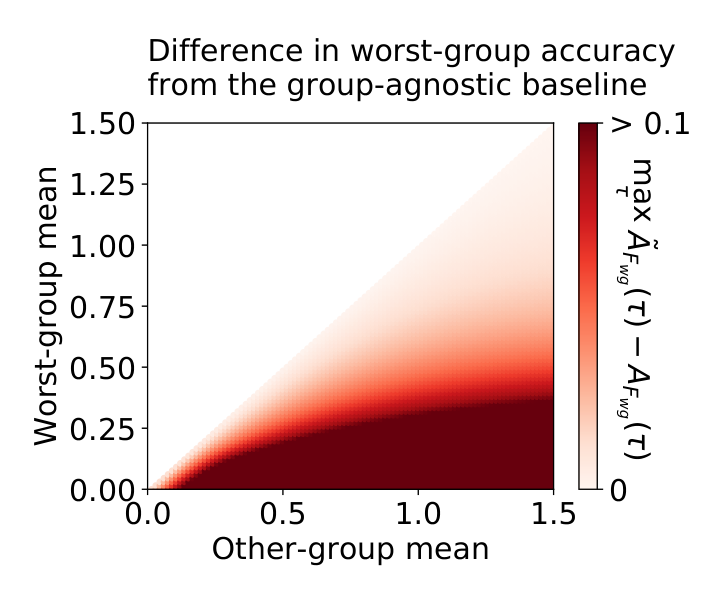
The RHS is the ratio of full-coverage errors; the larger the disparity between the worst group and the other groups at full coverage, the harder it is to satisfy this condition. In Appendix F, we simulate mixtures of Gaussians and show that this condition is rarely fulfilled.
Motivated by the empirical margin distributions, we apply Proposition 3 to the setting where and are both log-concave and are translated and scaled versions of each other. We show that the worst group must have lower variance than the others to outperform the group-agnostic reference:
Corollary 1 (Outperforming the group-agnostic reference requires smaller scaling for log-concave distributions).
Assume that , is log-concave, and for all , where is a scaling factor. If for all , .
This is consistent with the empirical margin distributions on Waterbirds: the worst group has higher variance, implying as is the ratio of the worst group’s standard deviation to the other group’s, and it thus fails to satisfy the necessary condition for outperforming the group-agnostic reference.
A further special case is when and are log-concave and unscaled translations of each other. Here, selective classification underperforms the group-agnostic reference at all thresholds .
Proposition 4 (Translated log-concave distributions underperform the group-agnostic reference).
Assume and are log-concave and for all . Then for all ,
| (6) |
This helps to explain our results on CheXpert-device, where the worst-group and average margin distributions are approximately translations of each other, and selective classification significantly underperforms the group-agnostic reference at all confidence thresholds.
7 Selective classification on group DRO models
Our above analysis suggests that selective classification tends to exacerbate group disparities, especially when the full-coverage disparities are large. This motivates a potential solution: by reducing group disparities at full coverage, models are more likely to satisfy the necessary condtion for outperforming the group-agnostic reference defined in Proposition 3. In this section, we explore this approach by training models using group distributionally robust optimization (group DRO) (Sagawa et al. 2020), which minimizes the worst-group training loss . Unlike standard training, group DRO uses group annotations at training time. As with prior work, we found that group DRO models have much smaller full-coverage disparities (Figure 5). Moreover, worst-group accuracies consistently improve as coverage decreases and at a rate that is comparable to the group-agnostic reference, though small gaps remain on Waterbirds and CheXpert-device.
While our theoretical analysis motivates the above approach, the analysis ultimately depends on the margin distributions of each group, not just on their full-coverage accuracies. Although group DRO only optimizes for similar full-coverage accuracies across groups, we found that it also leads to much more similar average and worst-group margin distributions compared to ERM (Figure 6), explaining why selective classification behaves more uniformly over groups across all datasets.
Group DRO is not a silver bullet, as it relies on group annotations for training, which are not always available. Nevertheless, these results show that closing full-coverage accuracy disparities can mitigate the downstream disparities caused by selective classification.
8 Discussion
We have shown that selective classification can magnify group disparities and should therefore be applied with caution. This is an insidious failure mode, since selective classification generally improves average accuracy and can appear to be working well if we do not look at group accuracies. However, we also found that selective classification can still work well on models that have equal full-coverage accuracies across groups. Training such models, especially without relying on too much additional information at training time, remains an important research direction. On the theoretical side, we characterized the behavior of selective classification in terms of the margin distributions; an open question is how different margin distributions arise from different data distributions, models, training procedures, and selective classification algorithms. Finally, in this paper we focused on studying selective accuracy in isolation; accounting for the cost of abstention and the equity of different coverages on different groups is an important direction for future work.
Acknowledgments
We thank Emma Pierson, Jean Feng, Pranav Rajpurkar, and Tengyu Ma for helpful advice. This work was supported by NSF Award Grant no. 1804222. SS was supported by the Herbert Kunzel Stanford Graduate Fellowship and AK was supported by the Stanford Graduate Fellowship.
Reproducibility
All code, data, and experiments are available on CodaLab at https://worksheets.codalab.org/worksheets/0x7ceb817d53b94b0c8294a7a22643bf5e. The code is also available on GitHub at https://github.com/ejones313/worst-group-sc.
References
- Azzalini & Regoli (2012) Adelchi Azzalini and Giuliana Regoli. Some properties of skew-symmetric distributions. Annals of the Institute of Statistical Mathematics, 64(4):857–879, 2012.
- Badgeley et al. (2019) Marcus A Badgeley, John R Zech, Luke Oakden-Rayner, Benjamin S Glicksberg, Manway Liu, William Gale, Michael V McConnell, Bethany Percha, Thomas M Snyder, and Joel T Dudley. Deep learning predicts hip fracture using confounding patient and healthcare variables. npj Digital Medicine, 2, 2019.
- Bagnoli & Bergstrom (2005) Mark Bagnoli and Ted Bergstrom. Log-concave probability and its applications. Economic Theory, 26:445–469, 2005.
- Balasubramanian et al. (2011) Krishnakumar Balasubramanian, Pinar Donmez, and Guy Lebanon. Unsupervised supervised learning II: Margin-based classification without labels. Journal of Machine Learning Research (JMLR), 12:3119–3145, 2011.
- Bartlett & Wegkamp (2008) Peter L Bartlett and Marten H Wegkamp. Classification with a reject option using a hinge loss. Journal of Machine Learning Research (JMLR), 9(0):1823–1840, 2008.
- Blodgett et al. (2016) Su Lin Blodgett, Lisa Green, and Brendan O’Connor. Demographic dialectal variation in social media: A case study of African-American English. In Empirical Methods in Natural Language Processing (EMNLP), pp. 1119–1130, 2016.
- Borkan et al. (2019) Daniel Borkan, Lucas Dixon, Jeffrey Sorensen, Nithum Thain, and Lucy Vasserman. Nuanced metrics for measuring unintended bias with real data for text classification. In World Wide Web (WWW), pp. 491–500, 2019.
- Boyd & Vandenberghe (2004) Stephen Boyd and Lieven Vandenberghe. Convex Optimization. Cambridge University Press, 2004.
- Buolamwini & Gebru (2018) Joy Buolamwini and Timnit Gebru. Gender shades: Intersectional accuracy disparities in commercial gender classification. In Conference on Fairness, Accountability and Transparency, pp. 77–91, 2018.
- Chen et al. (2020) Irene Y Chen, Emma Pierson, Sherri Rose, Shalmali Joshi, Kadija Ferryman, and Marzyeh Ghassemi. Ethical machine learning in health. arXiv preprint arXiv:2009.10576, 2020.
- Chow (1957) C. K. Chow. An optimum character recognition system using decision functions. In IRE Transactions on Electronic Computers, 1957.
- Chow (1970) Chao K Chow. On optimum recognition error and reject tradeoff. IEEE Transactions on Information Theory, 16(1):41–46, 1970.
- Corbett-Davies et al. (2017) Sam Corbett-Davies, Emma Pierson, Avi Feller, Sharad Goel, and Aziz Huq. Algorithmic decision making and the cost of fairness. In International Conference on Knowledge Discovery and Data Mining (KDD), pp. 797–806, 2017.
- Cordella et al. (1995) Luigi Pietro Cordella, Claudio De Stefano, Francesco Tortorella, and Mario Vento. A method for improving classification reliability of multilayer perceptrons. IEEE Transactions on Neural Networks, 6(5):1140–1147, 1995.
- Cule et al. (2010) Madeleine Cule, Richard Samworth, and Michael Stewart. Maximum likelihood estimation of a multi-dimensional log-concave density. Journal of the Royal Statistical Society, 73:545–603, 2010.
- De et al. (2020) Abir De, Paramita Koley, Niloy Ganguly, and Manuel Gomez-Rodriguez. Regression under human assistance. In Association for the Advancement of Artificial Intelligence (AAAI), pp. 2611–2620, 2020.
- Devlin et al. (2019) Jacob Devlin, Ming-Wei Chang, Kenton Lee, and Kristina Toutanova. BERT: Pre-training of deep bidirectional transformers for language understanding. In Association for Computational Linguistics (ACL), pp. 4171–4186, 2019.
- Dixon et al. (2018) Lucas Dixon, John Li, Jeffrey Sorensen, Nithum Thain, and Lucy Vasserman. Measuring and mitigating unintended bias in text classification. In Association for the Advancement of Artificial Intelligence (AAAI), pp. 67–73, 2018.
- Duchi et al. (2019) John Duchi, Tatsunori Hashimoto, and Hongseok Namkoong. Distributionally robust losses against mixture covariate shifts. https://cs.stanford.edu/~thashim/assets/publications/condrisk.pdf, 2019.
- Dwork et al. (2012) Cynthia Dwork, Moritz Hardt, Toniann Pitassi, Omer Reingold, and Rich Zemel. Fairness through awareness. In Innovations in Theoretical Computer Science (ITCS), pp. 214–226, 2012.
- El-Yaniv & Wiener (2010) Ran El-Yaniv and Yair Wiener. On the foundations of noise-free selective classification. Journal of Machine Learning Research (JMLR), 11, 2010.
- Feng et al. (2019) Jean Feng, Arjun Sondhi, Jessica Perry, and Noah Simon. Selective prediction-set models with coverage guarantees. arXiv preprint arXiv:1906.05473, 2019.
- Gal & Ghahramani (2016) Yarin Gal and Zoubin Ghahramani. Dropout as a Bayesian approximation: Representing model uncertainty in deep learning. In International Conference on Machine Learning (ICML), 2016.
- Geifman & El-Yaniv (2017) Yonatan Geifman and Ran El-Yaniv. Selective classification for deep neural networks. In Advances in Neural Information Processing Systems (NeurIPS), 2017.
- Geifman & El-Yaniv (2019) Yonatan Geifman and Ran El-Yaniv. Selectivenet: A deep neural network with an integrated reject option. In International Conference on Machine Learning (ICML), 2019.
- Geifman et al. (2018) Yonatan Geifman, Guy Uziel, and Ran El-Yaniv. Bias-reduced uncertainty estimation for deep neural classifiers. In International Conference on Learning Representations (ICLR), 2018.
- Gururangan et al. (2018) Suchin Gururangan, Swabha Swayamdipta, Omer Levy, Roy Schwartz, Samuel Bowman, and Noah A Smith. Annotation artifacts in natural language inference data. In Association for Computational Linguistics (ACL), pp. 107–112, 2018.
- Hanczar & Dougherty (2008) Blaise Hanczar and Edward R. Dougherty. Classification with reject option in gene expression data. Bioinformatics, 2008.
- Hardt et al. (2016) Moritz Hardt, Eric Price, and Nathan Srebo. Equality of opportunity in supervised learning. In Advances in Neural Information Processing Systems (NeurIPS), pp. 3315–3323, 2016.
- Hashimoto et al. (2018) Tatsunori B. Hashimoto, Megha Srivastava, Hongseok Namkoong, and Percy Liang. Fairness without demographics in repeated loss minimization. In International Conference on Machine Learning (ICML), 2018.
- He et al. (2016) Kaiming He, Xiangyu Zhang, Shaoqing Ren, and Jian Sun. Deep residual learning for image recognition. In Computer Vision and Pattern Recognition (CVPR), 2016.
- Hellman & Raviv (1970) Martin Hellman and Josef Raviv. Probability of error, equivocation, and the chernoff bound. IEEE Transactions on Information Theory, 16(4):368–372, 1970.
- Hellman (1970) Martin E Hellman. The nearest neighbor classification rule with a reject option. IEEE Transactions on Systems Science and Cybernetics, 6(3):179–185, 1970.
- Hendrycks & Gimpel (2017) Dan Hendrycks and Kevin Gimpel. A baseline for detecting misclassified and out-of-distribution examples in neural networks. In International Conference on Learning Representations (ICLR), 2017.
- Hill (2020) Kashmir Hill. Wrongfully accused by an algorithm. The New York Times, 2020. URL https://www.nytimes.com/2020/06/24/technology/facial-recognition-arrest.html.
- Hovy & Søgaard (2015) Dirk Hovy and Anders Søgaard. Tagging performance correlates with age. In Association for Computational Linguistics (ACL), pp. 483–488, 2015.
- Huang et al. (2017) Gao Huang, Zhuang Liu, Laurens Van Der Maaten, and Kilian Q Weinberger. Densely connected convolutional networks. In Proceedings of the IEEE Conference on Computer Vision and Pattern Recognition, pp. 4700–4708, 2017.
- Irvin et al. (2019) Jeremy Irvin, Pranav Rajpurkar, Michael Ko, Yifan Yu, Silviana Ciurea-Ilcus, Chris Chute, Henrik Marklund, Behzad Haghgoo, Robyn Ball, Katie Shpanskaya, et al. Chexpert: A large chest radiograph dataset with uncertainty labels and expert comparison. In Association for the Advancement of Artificial Intelligence (AAAI), volume 33, pp. 590–597, 2019.
- Joshi et al. (2018) Shalmali Joshi, Oluwasanmi Koyejo, Been Kim, and Joydeep Ghosh. xGEMs: Generating examplars to explain black-box models. arXiv preprint arXiv:1806.08867, 2018.
- Kamath et al. (2020) Amita Kamath, Robin Jia, and Percy Liang. Selective question answering under domain shift. In Association for Computational Linguistics (ACL), 2020.
- Khani et al. (2016) Fereshte Khani, Martin Rinard, and Percy Liang. Unanimous prediction for 100% precision with application to learning semantic mappings. In Association for Computational Linguistics (ACL), 2016.
- Kleinberg et al. (2017) Jon Kleinberg, Sendhil Mullainathan, and Manish Raghavan. Inherent trade-offs in the fair determination of risk scores. In Innovations in Theoretical Computer Science (ITCS), 2017.
- Koh et al. (2020) Pang Wei Koh, Shiori Sagawa, Henrik Marklund, Sang Michael Xie, Marvin Zhang, Akshay Balsubramani, Weihua Hu, Michihiro Yasunaga, Richard Lanas Phillips, Irena Gao, Tony Lee, Etienne David, Ian Stavness, Wei Guo, Berton A. Earnshaw, Imran S. Haque, Sara Beery, Jure Leskovec, Anshul Kundaje, Emma Pierson, Sergey Levine, Chelsea Finn, and Percy Liang. WILDS: A benchmark of in-the-wild distribution shifts. arXiv, 2020.
- Lakshminarayanan et al. (2017) Balaji Lakshminarayanan, Alexander Pritzel, and Charles Blundell. Simple and scalable predictive uncertainty estimation using deep ensembles. In Advances in Neural Information Processing Systems (NeurIPS), 2017.
- Liang et al. (2018) Shiyu Liang, Yixuan Li, and R. Srikant. Enhancing the reliability of out-of-distribution image detection in neural networks. In International Conference on Learning Representations (ICLR), 2018.
- Liu et al. (2015) Ziwei Liu, Ping Luo, Xiaogang Wang, and Xiaoou Tang. Deep learning face attributes in the wild. In Proceedings of the IEEE International Conference on Computer Vision, pp. 3730–3738, 2015.
- McCoy et al. (2019) R Thomas McCoy, Ellie Pavlick, and Tal Linzen. Right for the wrong reasons: Diagnosing syntactic heuristics in natural language inference. In Association for Computational Linguistics (ACL), 2019.
- Mozannar & Sontag (2020) Hussein Mozannar and David Sontag. Consistent estimators for learning to defer to an expert. arXiv preprint arXiv:2006.01862, 2020.
- Oakden-Rayner et al. (2020) Luke Oakden-Rayner, Jared Dunnmon, Gustavo Carneiro, and Christopher Ré. Hidden stratification causes clinically meaningful failures in machine learning for medical imaging. In Proceedings of the ACM Conference on Health, Inference, and Learning, pp. 151–159, 2020.
- Ovadia et al. (2019) Yaniv Ovadia, Emily Fertig, Jie Ren, Zachary Nado, D Sculley, Sebastian Nowozin, Joshua V. Dillon, Balaji Lakshminarayanan, and Jasper Snoek. Can you trust your model’s uncertainty? evaluating predictive uncertainty under dataset shift. In Advances in Neural Information Processing Systems (NeurIPS), 2019.
- Park et al. (2018) Ji Ho Park, Jamin Shin, and Pascale Fung. Reducing gender bias in abusive language detection. In Empirical Methods in Natural Language Processing (EMNLP), pp. 2799–2804, 2018.
- Pimentel et al. (2014) Marco AF Pimentel, David A Clifton, Lei Clifton, and Lionel Tarassenko. A review of novelty detection. Signal Processing, 99:215–249, 2014.
- Porcel (2018) José M Porcel. Chest tube drainage of the pleural space: a concise review for pulmonologists. Tuberculosis and Respiratory Diseases, 81(2):106–115, 2018.
- Raghu et al. (2019) Maithra Raghu, Katy Blumer, Rory Sayres, Ziad Obermeyer, Bobby Kleinberg, Sendhil Mullainathan, and Jon Kleinberg. Direct uncertainty prediction for medical second opinions. In International Conference on Machine Learning (ICML), pp. 5281–5290, 2019.
- Ribeiro et al. (2016) Marco Tulio Ribeiro, Sameer Singh, and Carlos Guestrin. ”Why Should I Trust You?”: Explaining the predictions of any classifier. In International Conference on Knowledge Discovery and Data Mining (KDD), 2016.
- Sagawa et al. (2020) Shiori Sagawa, Pang Wei Koh, Tatsunori B. Hashimoto, and Percy Liang. Distributionally robust neural networks for group shifts: On the importance of regularization for worst-case generalization. In International Conference on Learning Representations (ICLR), 2020.
- Tatman (2017) Rachael Tatman. Gender and dialect bias in YouTube’s automatic captions. In Workshop on Ethics in Natural Langauge Processing, volume 1, pp. 53–59, 2017.
- Toplak et al. (2014) Marko Toplak, Rok Močnik, Matija Polajnar, Zoran Bosnić, Lars Carlsson, Catrin Hasselgren, Janez Demšar, Scott Boyer, Blaz Zupan, and Jonna Stålring. Assessment of machine learning reliability methods for quantifying the applicability domain of QSAR regression models. Journal of Chemical Information and Modeling, 54, 2014.
- Wah et al. (2011) C Wah, S Branson, P Welinder, P Perona, and S Belongie. The Caltech-UCSD Birds-200-2011 dataset. Technical report, California Institute of Technology, 2011.
- Williams et al. (2018) Adina Williams, Nikita Nangia, and Samuel Bowman. A broad-coverage challenge corpus for sentence understanding through inference. In Association for Computational Linguistics (ACL), pp. 1112–1122, 2018.
- Wolf et al. (2019) Thomas Wolf, Lysandre Debut, Victor Sanh, Julien Chaumond, Clement Delangue, Anthony Moi, Pierric Cistac, Tim Rault, R’emi Louf, Morgan Funtowicz, and Jamie Brew. HuggingFace’s transformers: State-of-the-art natural language processing. arXiv preprint arXiv:1910.03771, 2019.
- Xiao et al. (2020) Kai Xiao, Logan Engstrom, Andrew Ilyas, and Aleksander Madry. Noise or signal: The role of image backgrounds in object recognition. arXiv preprint arXiv:2006.09994, 2020.
- Yu et al. (2011) Dong Yu, Jinyu Li, and Li Deng. Calibration of confidence measures in speech recognition. Trans. Audio, Speech and Lang. Proc., 19(8):2461–2473, 2011.
- Zhou et al. (2017) Bolei Zhou, Agata Lapedriza, Aditya Khosla, Aude Oliva, and Antonio Torralba. Places: A 10 million image database for scene recognition. IEEE Transactions on Pattern Analysis and Machine Intelligence, 40(6):1452–1464, 2017.
Appendix A Setup
A.1 Softmax response selective classifiers
In this section, we describe our implementation of softmax response (SR) selective classifiers (Geifman & El-Yaniv 2017). Recall from Section 3 that a selective classifier is a pair , where outputs a prediction and outputs the model’s confidence, which is always non-negative, in that prediction. SR classifiers are defined for neural networks (for classification), which generally have a last softmax layer over the possible classes. For an input point , we denote its maximum softmax probability, which corresponds to its predicted class , as . We defined the confidence for binary classifiers as
| (7) |
Since the maximum softmax probability is at least for binary classification, is nonnegative for each , and is thus a valid confidence. For classes, however, can be less than , in which case would be negative. To ensure that confidence is always nonnegative, we define for classes to be
| (8) |
With classes, the maximum softmax probability , and therefore we can verify that as desired. Moreover, when , Equation (8) reduces to our original binary confidence; we can therefore interpret the general form in Equation (8) as a normalized logit.
Note that is a monotone transformation of the maximum softmax probability . Since the accuracy-coverage curve of a selective classifier only depends on the relative ranking of across points, we could have equivalently set to be . However, following prior work, we choose the logit-transformed version to make the corresponding distribution of confidences easier to visualize (Balasubramanian et al. 2011; Lakshminarayanan et al. 2017).
Finally, we remark on one consequence of SR on the margin distribution for multi-class classification. Recall that we define the margin of an example to be on correct predictions () and otherwise, as described in Section 3. In Figure 4, we plot the margin distributions of SR selective classifiers on all five datasets. We observe that on MultiNLI, which is the only multi-class dataset (with ), there is a gap (region of lower density) in the margin distribution around 0. We attribute this gap in part to the comparative rarity of seeing a maximum softmax probability of when versus seeing when ; in the former, all three logits must be the same, while for the latter only two logits must be the same.
A.2 Group-agnostic reference
Here, we describe the group-agnostic reference described in Section 4 in more detail. We elaborate on the construction from the main text and then define the reference formally. Finally, we show that the group-agnostic reference satisfies equalized odds.
A.2.1 Definition
We begin by recalling on the construction described in the main text for a finite test set . In Algorithm 1 we relied on two important sets; the set of correctly classified points at threshold , :
| (9) |
and similarly, the set of incorrectly classified points at threshold , :
| (10) |
To compute the accuracy of the group-agnostic reference, we sample a subset of size uniformly at random from , and similarly a subset of size uniformly at random from . The group-agnostic reference makes predictions when examples are in and abstains otherwise. We compute group accuracies over this set of predicted examples.
Note that the group accuracies, as defined, are randomized due to the sampling. For the remainder of our analysis, we take the expectation over this randomness to compute the group accuracies. We now generalize the above construction by considering data distributions . We first define the number of correctly and incorrectly classified points:
Definition 3 (Correctly and incorrectly classified points).
Consider a selective classifier . For each threshold , we define the fractions of points that are predicted (not abstained on), and correctly or incorrectly classified, as
| (11) | ||||
| (12) |
We define analogous metrics for each group as
| (13) | ||||
| (14) |
For each threshold , we will make predictions on a fraction of the total (probability mass of) correctly classified points. Since each group has correctly classified points, at threshold , the group-agnostic reference will make predictions on correctly classified points in group . We can reason similarly over the incorrectly classified points. Putting it all together, we can define the group-agnostic reference as satisfying the following:
Definition 4 (Group-agnostic reference).
Consider a selective classifier and let , , , denote the analogous quantities to Definition 3 for its matching group-agnostic reference. For each threshold , these satisfy
| (15) | ||||
| (16) |
and for each threshold and group ,
| (17) | ||||
| (18) |
The group-agnostic reference thus has the following accuracy on group :
| (19) | ||||
| (20) |
A.2.2 Connection to equalized odds
We now show that the group-agnostic reference satisfies equalized odds with respect to which points it predicts or abstains on. The goal of a selective classifier is to make predictions on points it would get correct (i.e., ) while abstaining on points that it would have gotten incorrect (i.e., ). We can view this as a meta classification problem, where a true positive is when the selective classifier decides to make a prediction on a point and gets it correct (), and a false positive is when the selective classifier decides to make a prediction on a point and gets it incorrect (). As such, we can define the true positive rate and false positive rate of a selective classifier:
Definition 5.
The true positive rate of a selective classifier at threshold is
| (21) |
and the false positive rate at threshold is
| (22) |
Analogously, the true positive and false positive rates on a group are
| (23) | |||
| (24) |
The group-agnostic reference satisfies equalized odds (Hardt et al. 2016) with respect to this definition:
Proposition 5.
The group-agnostic reference defined in Definition 4 has equal true positive and false positive rates for all groups and satisfies equalized odds.
Proof.
By construction of the group-agnostic reference (Definition 4), we have that
| (25) | ||||
| (26) |
and therefore, for each group , we can show that the true-positive rate of the group-agnostic reference on is equal to its average true-positive rate .
| (27) | ||||
| (28) | ||||
| (29) |
Each group thus has the same true positive rate with the group-agnostic reference. Using similar reasoning, each group also has the same false positive rate. By the definition of equalized odds, the group-agnostic reference thus satisfies equalized odds. ∎
A.3 Robin Hood reference
| (30) |
Let be the accuracy of on points in that belong to group . We return the set that minimizes the difference between the best-group and worst-group accuracies.
| (31) |
In this section, we define the Robin Hood reference, which preferentially increases the worst-group accuracy through abstentions until it matches the other groups. Like the group-agnostic reference, we constrain the Robin Hood reference to make the same number of correct and incorrect predictions as a given selective classifier.
We formalize the definition of the Robin Hood reference in Algorithm 2. The Robin Hood reference makes predictions on the subset of examples from that has the smallest discrepency between best-group and worst-group accuracies, while still matching the number of correct and incorrect predictions of a given selective classifier. Since enumerating over all possible subsets of the test data is intractable, we compute the accuracies of the Robin Hood reference iteratively. Starting from full coverage, we abstain on examples from lowest to highest confidence. Whenever we abstain on an incorrect example, we assume it comes from the current lowest accuracy group, and similarly whenever we abstain on a correctly classified example we assume it comes from the current highest accuracy group. This reduces disparities to the maximum extent possible as the threshold increases.
Appendix B Supplemental experiments
B.1 Monte-Carlo dropout
In the main text, we observed that SR selective classifiers monotonically improve average accuracy as coverage decreases, but exacerbate accuracy disparities across groups on all five datasets. To demonstrate that these observations are not specific to SR selective classifiers, we now present our empirical results on another standard selective classification method: Monte-Carlo (MC) dropout (Gal & Ghahramani 2016; Geifman & El-Yaniv 2017). We find that MC-dropout selective classifiers exhibit similar empirical trends as SR selective classifiers.
MC-dropout selective classifiers. MC-dropout is an alternate way of assigning confidences to points. Taking a model with a dropout layer, the selective classifier first predicts simply by taking the model output without dropout. To estimate the confidence, it then samples softmax probabilities corresponding to the label over the randomness of the dropout layer. The confidence is computed as , where is the variance of the sampled probabilities. We implement MC-dropout by using the existing dropout layers for BERT and adding dropout to the final fully-connected layer for ResNet and DenseNet, with a dropout probability . We present empirical results for ; Gal & Ghahramani 2016 observed that this was sufficient to produce good confidence estimates.
Results. The MC-dropout selective classifiers exhibit similar trends to those that observed in Section 4, demonstrating that the observed empirical trends are not specific to SR response; even though the average accuracy improves monotonically as coverage decreases across all five datasets, the worst-group accuracy tends to decrease for CelebA, fails to increase consistently for CheXpert, Waterbirds, and CivilComments, and increases consistently but slowly for MultiNLI. Comparing SR and MC-dropout selective classifiers, we observe that the MC-dropout selective classifiers performs slightly worse. For example, we see a more prominent drop in worst-group accuracy for Waterbirds and much smaller improvements in worst-group accuracy for CheXpert.
B.2 Group DRO
We showed in Section 7 that SR selective classifiers trained with the group DRO objective successfully improve worst-group selective accuracies as coverage decreases, and perform comparably to the group-agnostic reference. We now present additional empirical results for these selective classifiers.
Accuracy-coverage curves.
We first present the accuracy-coverage curves for all groups, along with the group coverage trends, in Figure 8. Group selective accuracies tend to improve monotonically, in stark contrast with our results on standard (ERM) selective classifiers. These trends hold generally across groups and datasets, with a few exceptions; selective accuracies drop on two groups in MultiNLI at roughly 20% average coverage, and selective accuracies improve slowly on two groups in CivilComments. Below, we look into these anomalies and offer potential explanations.
For MultiNLI, we first note that the drops are observed at very low group coverages—lower than 1%—at which point the accuracies are computed based on very few examples and thus are noisy. In addition, much of the anomaly can be explained by label noise; we manually inspect the 20 examples from the above two groups with the highest softmax confidences, and find that 17 of them are labeled incorrectly. The observations on CivilComments can also be potentially attributed to label noise. Removing examples with high inter-annotator disagreement (with the fraction of toxic annotations between 0.5 and 0.6) yields an accuracy-coverage curve that fits the broader empirical trends.
Appendix C Experiment details
C.1 Datasets
CelebA.
Models have been shown to latch onto spurious correlations between labels and demographic attributes such as race and gender (Buolamwini & Gebru 2018; Joshi et al. 2018), and we study this on the CelebA dataset (Liu et al. 2015). Following Sagawa et al. 2020, we consider the task of classifying hair color, which is spuriously correlated with the gender. Concretely, inputs are celebrity face images, labels are hair color , and spurious attributes are gender, , with blondness associated with being female. Of the four groups, blond males are the smallest group, with only 1,387 examples out of 162,770 training examples, and they tend to be the worst group empirically. We use the official train-val-split of the dataset.
Waterbirds.
Object recognition models are prone to using image backgrounds as a proxy for the label (Ribeiro et al. 2016; Xiao et al. 2020). We study this on the Waterbirds dataset (Sagawa et al. 2020), constructed using images of birds from the Caltech-UCSD Birds dataset (Wah et al. 2011) placed on backgrounds from the Places dataset (Zhou et al. 2017). The task is to classify a photograph of a bird as one of , and the label is spuriously correlated with the background . Of the four groups, waterbirds on land backgrounds make up the smallest group with only 56 examples out of 4,795 training examples, and they tend to be the worst group empirically. We use the train-val-split provided by Sagawa et al. 2020, and also follow their protocol for computing average metrics; to compute average accuracies and coverages, we first compute the metrics for each group and obtain a weighted average according to group proportions in the training set, in order to account for the discrepancy in group proportions across the splits.
CheXpert-device.
Models can latch onto spurious correlations even in high-stakes applications such as medical imaging. When models are trained to classify whether a patient has certain pathologies from chest X-rays, models have been shown to spuriously detect the presence of a support device, in particular a chest drain, instead (Oakden-Rayner et al. 2020). We study this phenomenon in a modified version of the CheXpert dataset (Irvin et al. 2019), which we call CheXpert-device. Concretely, the inputs are chest X-rays, labels are , and spurious attributes indicate the the presence of a support device, . We note that chest drain is one type of support device, and is used to treat suspected pleural effusion (Porcel 2018).
CheXpert-device is a subsampled version of the full CheXpert dataset that manifests the spurious correlation more strongly. To create CheXpert-device, we first create a new 80/10/10 train/val/test split of examples from the publicly available CheXpert train and validation sets, randomly assigning patients to splits so that all X-rays of the same patient fall in the same split. We then subsample the training set; in particular, we enforce that in 90% of examples, the label of support device matches the pleural effusion label. Of the four groups, cases of pleural effusion without a support device make up the smallest group, with 5,467 examples out of 112,100 training examples, and they tend to be the worst group empirically.
To compute the average accuracies and coverages, we weight groups according to group proportions in the training set, similarly to Waterbirds. Another complication with CheXpert is that some patients can have multiple X-rays from one visit. Following Irvin et al. 2019, we treat these images as separate training examples at training time, but output one prediction for each patient-study pair at evaluation time. Concretely, we predict pleural effusion if the model detects the condition in any of the X-ray images belonging to the patient-study pair, as pathologies may only appear clearly in some X-rays.
CivilComments.
In toxicity comment detection, models have been shown to latch onto spurious correlations between the toxicity and mention of certain demographic groups (Park et al. 2018; Dixon et al. 2018). We study this in the CivilComments dataset (Borkan et al. 2019). The task is to classify the toxicity of comments on online articles with labels . As spurious attributes, we consider whether each comment mentions a Christian identity, ; non-toxicity is associated with the mention of Christian identity, often resulting in high false negative rate on comments with such mentions. Of the four groups, toxic comments with a mention of Christian identity make up the smallest group, with only 2,446 examples out of 269,038 training examples, and they tend to be the worst group empirically. and further split the development set into a training set and a validation set by randomly splitting on articles and associating all comments with each article to either set. We use the train, validation, and test set from the WILDS benchmark (Koh et al. 2020). The training, validation, and test set all comprise comments from disjoint sets of articles. The original dataset also contains many additional examples that have toxicity annotations but not identity annotations; we do not use these in our experiments.
In the original CivilComments dataset, each comment is given a probabilistic labels for both the toxicity and the mention of a Christian identity, where a probabilistic label is the average of binary labels across annotators. Following the associated Kaggle competition11 1 www.kaggle.com/c/jigsaw-unintended-bias-in-toxicity-classification/, we use binarized labels obtained by thresholding the probabilistic labels at 0.5.
MultiNLI. Lastly, we consider natural langage inference (NLI), where the task is to predict whether a hypothesis is entailed, contradicted by, or neutral to an associated premise, . NLI models have been shown to exploit annotation artifacts, for example predicting contradictory whenever negation words such as never or nobody are present (Gururangan et al. 2018). We study this on the MultiNLI dataset (Williams et al. 2018). To annotate examples’ spurious attributes , we consider the following negation words following Gururangan et al. 2018: “nobody”, “no”, “never”, and “nothing”. We use the splits used in Sagawa et al. 2020, whose training set includes 206,175 examples with 1,521 examples from the smallest group (entailment with negations). The worst group for standard models tends to be neutral examples with negation words.
C.2 Models
We train ResNet (He et al. 2016) for CelebA and Waterbirds (images), DenseNet (Huang et al. 2017) for CheXpert (X-rays), and BERT (Devlin et al. 2019) for CivilComments and MultiNLI (text). For tasks studied in Sagawa et al. 2020 (CelebA, Waterbirds, MultiNLI), we use the hyperparameters from Sagawa et al. 2020. For others (CivilComments and CheXpert-device), we test the same number of hyperparameter sets for each of ERM and DRO, and report the best set below. Across all image and X-ray tasks, inputs are downsampled to resolution 224 x 224.
CelebA. To train a model on CelebA, we initialize to pretrained ResNet-50. For ERM we optimize with learning rate 1e-4, weight decay 1e-4, batch size 128, and train for 50 epochs. For DRO we use learning rate 1e-5, weight decay 1e-1, and use generalization adjustment 1 (described in Sagawa et al. 2020). The batch size is 128, and we train for 50 epochs.
Waterbirds. For Waterbirds, as with CelebA, we use pretrained ResNet-50 as an initialization. For ERM we use learning rate 1e-3, weight decay 1e-4, batch size 128, and train for 300 epochs. For DRO we use learning rate 1e-5, weight decay 1, geneneralization adjustment 1, batch size 128, and train for 300 epochs.
CheXpert-device. For CheXpert-device, we fine-tune pretrained DenseNet-121 for three epochs. For ERM we use learning rate 1e-3, no weight decay, batch size 16, and choose the model (out of the first three epochs) with highest average accuracy (epoch 2). For DRO, we use learning rate 1e-4, weight decay 1e-1, and batch size 16, and choose the model with highest worst-group accuracy (epoch 1).
CivilComments. To train a model for CivilComments, we fine-tune bert-base-uncased using the implementation from Wolf et al. 2019. For both ERM and DRO we use learning rate 1e-5, weight decay 1e-2, and batch size 16. We train the ERM models and DRO models for three epochs (early stopping,) then choose the model with highest average accuracy for ERM (epoch 2), and highest worst-group accuracy for DRO (epoch 1).
MultiNLI. For MultiNLI we again fine-tune bert-base-uncased using the implementation from Wolf et al. 2019. For ERM, we fine-tune for three epochs with learning rate 2e-5, weight decay 0, and batch size 32. For DRO, we also use learning rate 2e-5, and weight decay 0, and batch size 32, but use generalization adjustment 1. For both ERM and DRO the model after the third epoch is best in terms of average accuracy for ERM and worst-group accuracy for DRO.
Appendix D Proofs: Margin distributions and accuracy-coverage curves
D.1 Left-log-concavity
Recall the definition of left-log-concave from Section 5: See 1 We first prove that a symmetric mixture of Gaussians is left-log-concave, but not necessarily log-concave.
D.1.1 Symmetric mixtures of Gaussians are left-log-concave
Lemma 1 (Symmetric mixtures of two gaussians are left-log-concave).
Consider a symmetric mixture of Gaussians with density , where is the density of a random variable and likewise is the density of a random variable. Then the mixture is left-log-concave for all values of , but only log-concave if .
Proof.
Without loss of generality, we can take , since (left-)log-concavity is invariant to scaling, and also assume that is positive. First consider the case where . Then the mixture is log-concave, and therefore left-log-concave (Cule et al. 2010).
Now, consider the case where . Cule et al. 2010 show the mixture is no longer log-concave. However, we claim that it is still left-log-concave. We start by studying the gradient of ,
| (32) | ||||
| (33) |
We claim that has a local minimum at , and as it is an odd function, a corresponding local maximum at . To show this, we first differentiate to obtain
| (34) |
Setting the derivative to 0 gives us the quadratic equation
| (35) | ||||||
| (36) | ||||||
| (37) | ||||||
| (38) | ||||||
Since , there are two distinct roots of this quadratic, and two corresponding critical points of . Let be the larger root. Then is a strictly increasing function for , and since , we have that for all . Let satisfy . Then we have that , the smaller of the critical points of , is
| (39) | ||||
| (40) | ||||
| (41) |
To show that is a local minimum, we take the second derivative
| (42) | ||||
| (43) |
which at gives
| (44) | ||||
| (45) |
since . Since is the only critical point of that is less than 0 and it is a local minimum, must be decreasing on , which in turn implies that , and therefore , is log-concave on .
It remains to show that is also log-concave on . We make use of two facts. First, since is a local minimum and the only critical point less than 0, we have that for all . Second, since and are non-negative for all , is also non-negative for all . Thus, for all
| (46) | ||||
| (47) | ||||
| (48) |
and therefore is also log-concave on . ∎
Remark 1.
Note that if is (left-)log-concave, then is also (left-)log-concave (Bagnoli & Bergstrom 2005). However, the reverse direction does not hold.
D.2 Symmetric margin distributions
In this section we prove Proposition 1. We first prove the following helpful lemma:
Lemma 2 (Conditions for monotonicity of selective accuracy).
is monotone increasing in if and only if
| (49) |
for all . Conversely, is monotone decreasing in if and only if the above inequality is flipped for all .
Proof.
is monotone increasing in if and only if for all . We obtain by differentiating and simplifying:
| (50) | ||||
| (51) | ||||
| (52) | ||||
| (53) |
Since the denominator is always positive, we have that if and only if the numerator , which in turn is equivalent to
| (54) |
as desired. The case for monotone decreasing is analogous. ∎
In the next two lemmas, we prove the necessary and sufficient conditions for Proposition 1 respectively.
Lemma 3 (Left-log-concavity and symmetry imply monotonicity.).
Let be symmetric about and let be left-log-concave. If , then is monotone increasing. Conversely, if , then is monotone decreasing.
Proof.
Consider the case where ; the case where is analogous. From Lemma 2 and the symmetry of , we have that is monotone increasing if (and only if)
| (55) |
holds for all .
To show that this inequality holds for all , we first note that since , we have that , which together with the symmetry of implies that . Thus, for all .
Now, if , then , so the desired inequality (55) follows from the log-concavity of on (Remark 1 of Bagnoli & Bergstrom 2005.)
Lemma 4 (Monotonicity and symmetry imply left-log-concavity.).
Let be symmetric with mean 0, and let be a translated version of that has mean . If is monotone increasing for all , then is left-log-concave.
Proof.
First consider . Since is monotone increasing for all , from Lemma 2 and the symmetry of ,
| (58) |
must hold for all . Since by construction, we can equivalently write
| (59) |
which holds for all as well, and by assumption, for all as well. By letting and , we can equivalently write the above inequality as
| (60) |
for all where .
By the definition of log-concavity, this means that is log-concave on . ∎
D.2.1 Left-log-concavity and monotonicity.
See 1
D.3 Skew-symmetric margin distributions
We now turn to how skew affects selective classification. Recall in Section 5 we defined skew-symmetric distributions as follows: See 2 When , and there is no skew. Increasing increases rightward skew, and decreasing increases leftward skew. Note that in general, the mean of depends on as well. We will also consider the translated distribution:
| (61) |
The CDF of is and the CDF of is . We will use the following properties of these distributions:
Lemma 5 (Skew-symmetry about ).
These properties hold when we flip the skew from to :
| (62) | ||||
| (63) |
Proof.
| (64) | ||||
| (65) | ||||
| (66) | ||||
| (67) | ||||
| (68) | ||||
| (69) | ||||
| (70) |
∎
Lemma 6 (Stochastic ordering with Proposition 4 from Azzalini & Regoli 2012).
Let . Then, for any , .
Proof.
Since the ordering is invariant to translation, without loss of generality we can take . First consider . Then
| (71) | ||||
| (72) | ||||
| (73) |
Now consider . We have
| (74) | |||||
| [by symmetry of G] | (75) | ||||
| (76) | |||||
| [by symmetry of h] | (77) | ||||
| [change of variables] | (78) | ||||
| (79) | |||||
which reduces to the case where . ∎
Lemma 7 (Log gradient ordering by skew).
For all , , and ,
| (80) |
Proof.
Since the ordering is invariant to translation, without loss of generality we can take . We have:
| (81) | ||||
| (82) | ||||
| (83) | ||||
| (84) | ||||
| (85) | ||||
| (86) |
To get the inequalities, note that when and , we have , since is an increasing function. Similarly, . Since is non-negative, the inequalities then follow from the monotonicity of the integral. ∎
We now prove the main results of this section.
D.3.1 Accuracy is monotone with skew
Proposition 6 (Accuracy is monotone with skew).
Let be the CDF of a skew-symmetric distribution. For all and , is monotonically increasing in .
Proof.
We use the skew-symmetry of to write the selective accuracy as
| (87) | ||||
| (88) |
We see that is a monotone decreasing function of . From Lemma 6, the numerator decreases with increasing while the denominator increases. Thus, this fraction decreases, which in turn implies that is monotone increasing with as desired. ∎
D.3.2 Skew in the same direction preserves monotonicity
See 2
Proof.
The idea is to use Lemma 7 to reduce the statement to the case where , so that we can apply monotonicity. First consider the case where is monotonically increasing in , and . We have
| [Lemma 7] | (89) | ||||
| [definition of ] | (90) | ||||
| [from monotonicity of (Lemma 2)] | (91) | ||||
| [symmetry of ] | (92) | ||||
| [definition of ] | (93) | ||||
| [Lemma 7] | (94) | ||||
| [Lemma 5] | (95) |
Applying Lemma 2 completes the proof. The case where is analogous. ∎
D.4 Monotone odd transformations preserve accuracy-coverage curves.
We now show that our results are unchanged by strictly monotone and odd transformations to the density.
Lemma 8 (Odd and strictly monotonically increasing transformations preserve selective accuracy).
Let be a real-valued random variable with CDF , be a strictly monotonically increasing function, and define random variable with CDF . Then, for each .
Proof.
For each , since is a strictly monotonically increasing function, we apply the change of variables formula for transformations of univariate random variables to get the following:
| (96) | |||||
| [ is odd] | (97) | ||||
We now solve for selective accuracy:
| (98) | ||||
| (99) | ||||
| (100) |
∎
With Lemma 8, our results extend all random variables where corresponds to a left-log-concave distribution and is odd and strictly monotonically increasing. In particular, and have the same accuracy-coverage curves.
Appendix E Proofs: Comparison to the group-agnostic reference
In this section, we present the proofs from Section 6, which outline conditions under which selective classifiers outperform the group-agnostic reference.
E.1 Definitions
We first define certain metrics on selective classifiers and their group-agnostic reference in terms of their margin distributions.
Definition 6.
Consider a margin distribution with CDF
| (101) |
where is the mixture weight and is the CDF for group . We write the fraction of examples that are correct/incorrect and predicted on at threshold from group and on average as follows:
| (102) | ||||
| (103) | ||||
| (104) | ||||
| (105) |
We write the true-positive rate and false-positive rate for a given threshold as
| (106) | ||||
| (107) |
Finally, we write the accuracy of the group-agnostic reference on group as
| (108) | ||||
| (109) |
For convenience in our proofs below, we also define the fraction of each group in correctly and incorrectly classified predictions at each threshold .
Definition 7.
We define the fraction of group out of correctly and incorrectly classified predictions at threshold , and respectively, as
| (110) | ||||
| (111) |
E.2 General necessary conditions to outperform the group-agnostic reference
We first write the accuracy of the group-agnostic reference in terms of and .
Lemma 9.
| (112) |
Proof.
We have:
| (113) | ||||
| (114) | ||||
| (115) | ||||
| (116) | ||||
| (117) |
∎
Lemma 10 (Bounding the derivative of at ).
If ,
| (118) |
Proof.
| (119) | |||||
| (120) | |||||
| (121) | |||||
| (122) | |||||
| (123) | |||||
| (124) | |||||
| (125) | |||||
| (126) | |||||
| (127) | |||||
| (128) | |||||
∎
Lemma 11.
If , then
| (129) |
for some positive constant .
E.2.1 Necessary condition for outperforming the group-agnostic reference
See 3
Proof.
Recall that
| (138) | ||||
| (139) |
If for all , then
| (140) |
From Lemma 11,
| (141) |
for some positive constant . Combined,
| (142) |
∎
E.2.2 Outperforming the group-agnostic reference requires smaller scaling for log-concave distributions
See 1
Proof.
By Proposition 3, if for all , then:
| (143) |
and equivalently,
| (144) |
From the definition of ,
| (145) |
Because , . Applying log-concavity yields
| (146) |
Thus, when , there exists some threshold where . ∎
E.3 Translated, log-concave distributions always underperform the group-agnostic reference
We now present a proof of Proposition 4. Assume and are log concave and symmetric, the worst group has mean , the combination of other group(s) has mean , and , (the densities are translations of each other.) For convenience, define . This implies:
| (147) | ||||
| (148) |
We will first show that is indeed the worst group at full coverage; i.e. :
Lemma 12.
If is a PDF and is obtained by translating to the right (i.e. for ), and and are their associated CDFs, .
Proof.
We have:
| (149) | ||||
| (150) | ||||
| (151) | ||||
| (152) |
∎
We next show that is monotonically decreasing in :
Lemma 13.
If , , , , , and are as described, is monotonically decreasing in .
Proof.
First, defining in terms of , we have:
| (153) | ||||
| (154) | ||||
| (155) | ||||
| (156) |
Taking the derivative of , we have:
| (157) | ||||
| (158) | ||||
| (159) |
where is a positive constant (since and are positive and all of the terms are squares.) Thus, we can say that is monotonically decreasing for all if:
| (160) | |||
| (161) |
Now, since , this follows from the log concavity of . Therefore, the fraction of correct examples that come from group is a decreasing function of . ∎
Next, we show that the is monotonically increasing in :
Lemma 14.
If , , , , and are as described, is monotonically increasing in .
Proof.
First, we note that:
| (162) | ||||
| (163) |
We will show that the derivative of with respect to is positive. Doing so gives us:
| (164) | ||||
| (165) | ||||
| (166) |
where is positive since it is the product of squared terms and , which is also positive. Thus, is equivalent to:
| (167) | ||||
| (168) | ||||
| (169) |
Since is log-concave and is positive, the last inequality is true, so is monotonically increasing in , as desired. ∎
Lemma 15.
is monotonically increasing in
Proof.
We will now prove the main result of this section:
E.3.1 Translated, log-concave distributions always underperform the group-agnostic reference
See 4
Proof.
We consider the case of underperforming the group-agnostic reference: the case of overperforming the group-agnostic reference is analogous. Assume the worst group is the lower accuracy group (so is positive.) Using the definition of selective accuracy, we have:
| (172) | |||||
| (173) | |||||
| (174) | |||||
| [by Lemma 15] | (175) | ||||
| (176) | |||||
| (177) | |||||
Thus, the worst group underperforms the group-agnostic reference, as desired. ∎
Appendix F Simulations
To demonstrate that it is possible but challenging to outperform the group-agnostic reference, we present simulation results on margin distributions that are mixtures of two Gaussians. Following the setup from Section 6, we consider a best-group margin distribution and a worst-group margin distribution varying the parameters . We set the fraction of mass from the worst group, to be 0.5. We evaluate whether selective classification outperforms the group-agnostic reference, plotting the results in Figure 9. We observe that selective classification outperforms the group-agnostic reference under some parameter settings, notably when the necessary condition in Proposition 3 is met and when the variance is smaller as implied by Corollary 1, but it underperforms the group-agnostic reference under most parameter settings.
In addition to whether the worst group underperforms or outperforms the group-agnostic reference, we study the magnitude of the difference in the worst-group accuracy with respect to the group-agnostic reference through the same simulations (Figure 10). Concretely, we compute the difference in worst-group accuracy with respect to the group-agnostic reference, taking the worst-case difference across thresholds: . We observe significant disparities between the observed worst-group accuracy and the group-agnostic reference.

Lastly, we simulate the effects of varying the worst-group and other-group means while keeping the variance fixed at for both groups, following the same simulation protocol otherwise. We similarly observe substantial gaps between the observed worst-group accuracy and the group-agnostic reference (Figure 11).