Developing Univariate Neurodegeneration Biomarkers with Low-Rank and Sparse Subspace Decomposition
Abstract
††footnotetext: Data used in preparation of this article were obtained from the Alzheimer’s Disease Neuroimaging Initiative (ADNI) database (adni.loni.usc.edu). As such, the investigators within the ADNI contributed to the design and implementation of ADNI and/or provided data but did not participate in analysis or writing of this report. A complete listing of ADNI investigators can be found at: https://adni.loni.usc.edu/wp-content/uploads/how_to_apply/ADNI_Acknowledgement_List.pdfE-mail: ylwang@asu.edu, gangwang1970@ldu.edu.cn
Cognitive decline due to Alzheimer’s disease (AD) is closely associated with brain structure alterations captured by structural magnetic resonance imaging (sMRI). It supports the validity to develop sMRI-based univariate neurodegeneration biomarkers (UNB). However, existing UNB work either fails to model large group variances or does not capture AD dementia (ADD) induced changes. We propose a novel low-rank and sparse subspace decomposition method capable of stably quantifying the morphological changes induced by ADD. Specifically, we propose a numerically efficient rank minimization mechanism to extract group common structure and impose regularization constraints to encode the original 3D morphometry connectivity. Further, we generate regions-of-interest (ROI) with group difference study between common subspaces of AD and cognitively unimpaired (CU) groups. A univariate morphometry index (UMI) is constructed from these ROIs by summarizing individual morphological characteristics weighted by normalized difference between AD and CU groups. We use hippocampal surface radial distance feature to compute the UMIs and validate our work in the Alzheimer’s Disease Neuroimaging Initiative (ADNI) cohort. With hippocampal UMIs, the estimated minimum sample sizes needed to detect a 25 reduction in the mean annual change with 80 power and two-tailed are 116, 279 and 387 for the longitudinal AD, mild cognitive impairment (MCI) and CU groups, respectively. Additionally, for MCI patients, UMIs well correlate with hazard ratio of conversion to AD (, CI=) within 18 months. Our experimental results outperform traditional hippocampal volume measures and suggest the application of UMI as a potential UNB.
Keywords:
Magnetic resonance imaging (MRI), Alzheimer’s disease, Subspace decomposition, Univariate morphometry index, Minimum sample size, Cox proportional hazard model1 Introduction
Alzheimer’s disease (AD) is a progressive neurodegenerative disease and also the most common type of dementia. Its prevalence is predicted to triple to 13.8 million by 2050. It is generally agreed that effective diagnosis and treatment of AD could have enormous public health benefits. Prior research on structural magnetic resonance imaging (sMRI) supported its validity as a potential noninvasive neurodegeneration biomarker of AD (Frisoni et al. 2010; Sperling et al. 2011; Jack et al. 2016; Zhao et al. 2017). Such sMRI-based imaging biomarkers will facilitate the development of effective interventions that may postpone (or prevent) symptomatic AD (Caselli and Reiman 2013; Langbaum et al. 2013).
Structural MRI-based measures of atrophy including whole brain (Fox et al. 1999; Chen et al. 2007; Stonnington et al. 2010), entorhinal cortex (Cardenas et al. 2011), hippocampus (Jack et al. 2003; Thompson et al. 2004; den Heijer et al. 2010; Wang et al. 2011; Dong et al. 2019) and temporal lobe volumes (Hua et al. 2010), as well as ventricular enlargement (Jack et al. 2003; Thompson et al. 2004; Wang et al. 2011; Dong et al. 2020), correlate closely with changes in cognitive performance, inspiring various neuroimaging biomarker approaches. Among them, hippocampal atrophy measures from sMRI are widely used, as hippocampal morphometry changes are apparent in the early stages of memory decline and may anticipate progression to mild cognitive impairment (MCI) and AD (Jack et al. 2003).
While much AD imaging biomarker research has been devoted to group difference-based analyses, a univariate neurodegeneration biomarker (UNB) based on an individual patient’s brain scans with high diagnostic accuracy would be highly desirable for clinical use (Sabuncu et al. 2016). Such a personalized measure may overcome inflated Type I error due to multivariate comparisons. For example, for randomized clinical trials (RCT), regulatory agencies, including the Food and Drug Administration (FDA), requires conventional univariate hypothesis testing and its associated statistical power analysis (Langbaum et al. 2013). Meanwhile, a single MRI-based measure of cerebral atrophy was used as a neurodegeneration biomarker in the recently proposed AD amyloid/tau/neurodegeneration (A/T/N) framework (Jack et al. 2016). It is a descriptive system for categorizing multidomain biomarker findings at the individualized level in a format that is easy to understand and use. Rather than conceptualizing AD primarily as a clinicopathological entity, in this system AD is diagnosed using biomarkers such as brain imaging or by measuring substances in the cerebral spinal fluid. This change may allow preclinical AD diagnosis on presymptomatic patients (Knopman et al. 2018). However, a recent work (Illan-Gala et al. 2018) reported that the currently available neurodegeneration biomarkers, including hippocampal volume and cortical signature of AD (Dickerson et al. 2009), were poorly correlated both in their whole dataset and along the AD continuum. Therefore, to advance computational neuroanatomy to clinical usage, developing a robust method to quantify brain sMRI difference using a statistically powerful UNB will be highly advantageous for clinical diagnosis and prognosis.
In the past decade, a variety of univariate morphological MRI biomarker algorithms have been developed (Racine et al. 2018; Cardenas et al. 2011; Cortechs Labs 2020; Vemuri et al. 2008; Tu et al. 2020, e.g.). Meanwhile, a few multivariate analysis frameworks (Hua et al. 2011; Gutman et al. 2013) took statistical or machine learning approaches to optimize the minimum sample size estimation for clinical trials. Among them, most are based on regions-of-interest (ROI) analyses and obtain a UNB by summarizing image information from these ROIs. Such methods enjoy good biological interpretability and excellent computational efficiency. However, there are a number of issues: (1) In their modeling, such approaches do not take into account the strong noise and the large within-group variance on the obtained sMR images; (2) When setting up training data, they usually use the clinical symptom-based AD diagnosis without the confirmation of imaging or fluid information. These difficulties have largely limited the statistical power and generalibility of their UNB due to excessive imaging noise, strong individual morphological differences and the inhomogeneity of dementia.
To address these challenges, it is important to generate reliable and robust sMRI ROIs that reflect intrinsic structural differences caused by AD dementia (ADD). Recently, research on low-rank and sparse subspace decomposition by rank minimization and sparse constraint has attracted strong interest (Cao et al. 2017; Jang et al. 2016; Javed et al. 2016). In particular, robust principal component analysis (RPCA) (Candès et al. 2011) through principal component pursuit (PCP) decomposes a data matrix into two subspaces which include a low-rank component and a sparse component. The low-rank subspace may mine the common structure belonging to a specific group, and the sparse component can detect salient features belonging to a specific individual (Hastie et al. 2015). When individual brain image measurements of the same group subjects are stacked into columns to generate the group observation matrix, we may expect its low-rank components correspond to the group common structure. Except for this group common structure, individual image differences correspond to the sparse component. Furthermore, one of the hallmarks of AD is the accumulation of beta-amyloid plaques () in human brains and a positive reading is now accepted as ‘dementia due to AD’ together with the presence of clinical symptoms. In this paper, we propose a novel subspace decomposition-based method to generate the ROIs based on the group difference from extracted low-rank components of positive AD and negative cognitively unimpaired (CU) groups and later define a univariate neurodegeneration biomarker, univariate morphometry index (UMI), which may reflect intrinsic morphological changes induced by ADD and also have strong generalization ability on new subjects. Previous research (Thompson et al. 2004; Apostolova et al. 2010; Qiu et al. 2010; Costafreda et al. 2011; Dong et al. 2019, e.g.) has demonstrated that surface-based hippocampal morphometry analysis offers advantages over volume measures. Therefore, we apply our subspace decomposition method to hippocampal measures obtained with our prior hippocampal morphometry study (Shi et al. 2013) to construct UMIs. We hypothesize that our low-rank and sparse subspace decomposition framework together with surface-based measures may be used to compute robust and efficient UNBs and improve their statistical power compared with the traditional univariate biomarker, such as hippocampal volumes (Jack et al. 2003; Cortechs Labs 2020). Here, we set out to validate our hypothesis on brain sMR images from the Alzheimer’s Disease Neuroimaging Initiative (ADNI) cohort.
2 Material and Methods
2.1 Subjects
Data is downloaded from the Alzheimer’s Disease Neuroimaging Initiative (ADNI) database ((Mueller et al. 2005), adni.loni.usc.edu). ADNI is the result of efforts of many co-investigators from a broad range of academic institutions and private corporations. Subjects have been recruited from over 50 sites across the U.S. and Canada. The primary goal of ADNI is to test whether biological markers, such as serial MRI and positron emission tomography (PET), combined with clinical and neuropsychological assessments, can measure the progression of MCI and early AD. Subjects originally recruited for ADNI-1 and ADNI-GO had the option to be followed in ADNI-2. For up-to-date information, see www.adniinfo.org.
In this study, we use brain structural MRI data from A positive () AD patients and A negative () CU to identify the ROIs which are further used to define UMI. To validate our algorithm, we study (1) longitudinal brain imaging changes via group difference and minimum sample size estimation; and (2) future clinical decline prediction for MCI patients via survival analysis. In the first experiment, we use structural MRI data from longitudinal subjects, including AD, MCI and CU subjects. All subjects of each longitudinal group underwent two tests, including the baseline test and a 24-months test. In the second experiment, we use MCI patients including MCI subjects who have converted to probable AD and non-converter MCI subjects within 18-months period.
2.2 System Pipeline Overview

Here we briefly overview the processing pipeline in our univariate morphometry index (UMI) system. Following sections are detailed explanations of each step. The pipeline code is publicly available at https://gsl.lab.asu.edu/software/univariate-neurodegeneration
-biomarkers.
Fig. 1 summarizes the overall sequence of steps in the system. First, we reconstruct hippocampal surfaces after we segment hippocampi from T1-weighted MR images. We register hippocampal surfaces across subjects and compute surface morphometry features, radial distance (RD) (Pizer et al. 1999; Styner et al. 2006; Thompson et al. 2004) (the first row, Fig. 1). Second, we build group morphometry (i.e., radial distance - RD) observation matrices, i.e., the observation matrix of A positive () AD group and the observation matrix of A negative () CU group, where each individual RD features are concatenated as a column vector. Due to the morphological similarity within the same group, we further decompose each group RD matrix into low-rank component and sparse component based on the matrix factorization with orthogonal constraint and sparsity shrinkage strategy (the second row, Fig. 1). Third, with group difference study, we identify significantly different areas between the low rank components of two groups, AD group and CU group, as the regions-of-interest (ROI) and use them as the significant morphological change regions induced by ADD (the third row, Fig. 1). Finally, based on the registration result of an individual hippocampal surface, the UMI of the individual subject is computed through the voxel-wise AD atrophy degrees and the individual atrophy degrees defined on the ROIs (Sec. 2.5). As applications of the computed UMIs, we apply them to three different studies, including longitudinal analysis, sample size estimation, and progression rate predictions from MCI to probable AD (the fourth row, Fig. 1)
2.3 Image Acquisition and Hippocampal Morphometry Surface Feature Computation
High-resolution brain structural MRI scans are acquired at multiple ADNI sites using 1.5 Tesla MRI scanners manufactured by General Electric Healthcare, Siemens Medical Solutions, and Philips Medical Systems. For each subject, the T1-weighted MRI scan is collected with a sagittal 3D MP-RAGE sequence. Typical T acquisition parameters are repetition time (TR) of ms, minimum full excitation time (TE), inversion time (TI) of ms, flip angle of , cm field of view. The acquisition matrix is in the x, y, and z dimensions and the voxel size is . In-plane, zero-filled reconstruction (i.e., sinc interpolation) generate a matrix for a reconstructed voxel size of .
The hippocampal substructures are segmented with FIRST (Patenaude et al. 2011) based on the T1-weighted MRI scans, and hippocampal surfaces are automatically reconstructed based on the segmentations (Han et al. 2003; Lorensen and Cline 1987). To overcome the noise caused by the image scanning and the partial volume effects, a smoothing process consisted of two steps, i.e., progressive meshes (Hoppe 1996) and loop subdivision(Loop 1987), is applied to the reconstructed hippocampal surfaces. A nonlinear surface registration method, inverse consistent fluid registration method (Shi et al. 2013), is applied to register individual hippocampal surfaces to a standard template surface by constrained harmonic maps. After the registration, surface deformation statistics are computed to obtain the radial distance (RD) (Pizer et al. 1999; Styner et al. 2006; Thompson et al. 2004) represented as the shortest distance from each surface vertex to the medical axis of a tube-shape surface. For the following subspace decomposition analysis, we represent an individual’s RD features as a column vector and concatenate them to construct group morphometry observation matrices.
2.4 Low-Rank and Sparse Subspace Decomposition Algorithm
Based on the robust principal component analysis (RPCA) (Candès et al. 2011), the low-rank component and the sparse component in a morphological observation matrix ( is the dimension of the biomarker and is the number of the subjects) can be extracted through a convex optimization procedure. The low-rank component is the group common structure contributed by all the individuals in the same group, and the sparse component is the sparse characteristics which belong to specific individual subjects. In practice, the observation matrix is usually corrupted by noise which can affect every data matrix entry and lead to analysis errors. To solve this problem and achieve a stable separation, a convex model called stable principal component pursuit (SPCP) (Zhou et al. 2010) has been proposed. This model may guarantee a stable recovery of and with an error bound proportional to the overall noise magnitude . The solution to SPCP can be formulated by the following equation,
| (1) |
In Eq. 1, is the nuclear norm and is the -norm, given by , respectively, where is the vector of singular values of , the controls the relative importance of the low-rank component vs. the sparse component . The noise is implicit in the equation, i.e., . Since SPCP algorithm involves minimizing a combination of -norm and nuclear norm, the singular value decomposition (SVD) step included in the nuclear norm makes the convergence of SPCP optimization problem very slow, especially for large-scale observation matrices (Tseng 2008; Lin et al. 2009). To reduce the SVD computation cost for a large-scale matrix, we adopt a low-rank matrix factorization mechanism (Liu and Yan 2012) to factorize a large-sized matrix into the product of two small-sized matrices. Because the group common structure is of low-rank, can be factorized into the product of two small-sized matrices, i.e., . Then we obtain by enforcing to be column orthonormal, i.e., , is the identity matrix. Thus, Eq. 1 can be transformed into an optimization problem constrained on a small-scale matrix,
| (2) |
Since any low-rank matrix can be factorized into a product of two small-sized matrices with , this transformation significantly speeds up the SPCP optimization for large-scale matrices.
To extract the sparse component without loss of the original spatial information, we define as continuous patches in local regions. We further propose a novel formulation which considers the original spatial distribution of the sparse morphological component . Supposing we have an observation data matrix , and where denotes the column vector of the original morphological measurements of -th subject. In order to detect the local continuous characteristics, we enforce a local sparse measure for every column in the observation matrix, defined as follows:
| (3) |
where is the number of the row in the observation matrix and is the vertex sequence number in the triangular mesh of the specific subject. And denotes the one-ring area centered on the vertex , is the Hadamard product, is the shrinking function and is the threshold. By using to replace the -norm constraint in Eq. 2, and representing the local spatial continuous characteristics of the salient features, Eq. 2 can be modified as,
| (4) |
Given the well-known alternating direction method and the Douglas-Rachford operator splitting (DR) method (Douglas and Rachford 1956), the minimization task of the Eq. 4 can be decomposed into three simpler tasks which solve the variables separately in a consecutive order. Let be the Lagrange multiplier associated with the linear constraint in Eq. 4, the augmented Lagrangian function of Eq. 4 is:
| (5) |
Based on the DR method, let , the according iteration procedure for Eq. 5 is described as follows:
| (6) |
The generated subproblems in Eq. 6 admit analytic solutions. The first subproblem involving can be solved explicitly via:
| (7) |
where . Note that the computation complexity for this subproblem is . For the second subproblem involving in Eq. 6, it is equivalent to solve the following equation.
| (8) |
Denoting , and substituting for in Eq. 3. The following formulation gives a closed-form solution of the minimization with respect to
| (9) |
Here is the result matrix which is the in Eq. 3. Therefore, Eq. 9 sets the pixels of to be zero value if the corresponding is less than , or shrinks the corresponding pixel by a factor . After an iteration of update, we obtain terms. Denote , and the known condition . To acquire the with column orthonormal and with a small scale, we chose two-steps. First, we fix the and compute the . According to Higham and Papadimitriou 1995, the update of is given by the following equation,
| (10) |
For a given matrix , SVD can be applied to and the result is . Therefore the operator can be defined as . It can be verified that is always column orthonormal (i.e., ). Through Eq. 10, we can get the by satisfying the condition (i.e., ). Second, fixing and computing the , the update of is as follows,
| (11) |
For a given matrix , , the solution of minimizing of the nuclear norm of is given by , defined by
| (12) |
where , and are obtained by the singular value decomposition (SVD) of , and (Cai et al. 2008). Here . Thus, according to Eq. 10 and Eq. 11 , the solution of in Eq. 6 can also be solved by
| (13) |
With Eq. 10 and Eq. 11, the SVD computation complexity is reduced from to . In addition, we set the parameters in Eq. 5 as , where and represent the numbers of rows and columns in the observation data matrix. The parameter . The is the largest singular value of the observation data matirx and . And the parameter in Eq. 1 is set as (Tao and Yuan 2011), is the standard deviation of the observation data matrix. Finally, the algorithm is terminated when . Based on the above description, we can use the proposed method to efficiently and accurately recover the low-rank component and the sparse component with a local continuous constraint from the large-scale data matrix in a complicated environment. In particular, we can use the low-rank component, i.e., where denotes the group common structure, to study the group differences without considering the individual specific diversities in .
2.5 Univariate Morphometry Index (UMI)
Taking the morphological RD measures on the hippocampal surfaces as features, we apply the subspace decomposition algorithm to analyze data from both AD and CU groups and obtain the essential group common morphological structures from the individuals of the same group, i.e., s of AD group and CU group, while discarding the within-group morphological differences and the noise. Using the two group common morphological structures, the ROIs are generated through group difference analysis. This means that the generated ROIs reflect the hippocampal morphological structure changes from CU to AD. Next, we obtain the voxel-wise AD atrophy degrees by normalizing the mean differences between the of A AD group and the of A CU group in the predefined ROIs. The individual atrophy degree can be computed in the predefined ROIs by normalizing the differences between the RD vector of an individual subject and the low-rank component mean of the A CU group. Last, the UMIs can be obtained through the voxel-wise summation across all the voxels on the predefined ROIs with the production of AD atrophy degrees and the individual atrophy degree:
| (14) |
where is the total number of voxels in the predefined ROI, denotes the atrophy degree at voxel of the testing individual (defined as the mean of the A negative CU group subtracted by the individual RD on the predefined ROI), and is the atrophy degree at voxel (defined as the difference of the mean of A AD group and the mean of A CU group on the predefined ROI). From Eq. 14, we see that the UMIs measure how similar the individual atrophy degree is when compared to the AD atrophy degree in the selected ROIs, similar to our previous work (Chen et al. 2011). In other words, the greater the UMIs, the closer the individual atrophy degree from the AD morphological characteristics.
2.6 Assessments of Univariate Morphometry Index
2.6.1 Group Comparisons
We compare the group mean differences for the UMI results of different longitudinal A groups based on the paired -test, including longitudinal A AD, A MCI and A CU groups. All subjects of each longitudinal group underwent two tests, including the baseline test and a 24-months test. We use Cohen’s d test to evaluate the effect size. Cohen’s d test takes the difference in means between two groups and is devided by the pooled standard deviation of the groups. For MCI converters and non-converters within 18-months period, we analyze the group differences of the UMI measures, Mini-Mental State Examination (MMSE) (Folstein et al. 1975) scores, Auditory Verbal Learning Test Total (AVLT-Total) (Rey 1964) scores and hippocampal volume measurements by using analysis of variance (ANOVA) method to compare their statistical discrimination abilities .
2.6.2 Minimum Sample Size Estimation for Longitudinal Study
To assess the statistical power of the defined UMI, we study the minimum sample size estimation, i.e., with 80 power and a 25 reduction in the mean annual change, using a two-sided test and standard significance level for a hypothetical two-arm study (treatment vs. placebo, as advocated by the ADNI Biostatistics Core) (Beckett et al. 2010) for longitudinal (baseline and 24-months follow-up) studies. The minimum sample size is computed from the below formula:
| (15) |
where denotes the standard deviation of the biomarkers’ changes, and refer to the mean value of the biomarkers at the time and of the longitudinal data. is a constant. If the minimum sample size derived from a biomarker was smaller than that of another biomarker , we may conclude that biomarker has more differentiation ability than biomarker . It suggests that minimum sample size is an indicator for characterizing the statistical power of biomarkers.
2.6.3 Prediction Rates of Progression from MCI to probable AD
We compare UMIs, hippocampal volume measurements and AVLT-Total scores in their abilities to predict rates of conversion from MCI to AD within the 18-months period after baseline. We initially use Receiver Operating Characteristic (ROC) analyses to determine the measurement cut-offs with optimal sensitivity and specificity for distinguishing between the MCI converters and those who are stable. The nearest point method is used to find the cut-offs on the ROC curve closest to (0,1), that is, the point with optimal sensitivity and specificity. The cut-offs are used to compare the MCI patients with or without a positive test score (i.e., those with or without a higher UMI, lower hippocampal volume or lower AVLT-Total score) in the hazard ratio of converting from MCI to AD within 18-months period. We also report area under the curve (AUC), which is an effective and combined measure of sensitivity and specificity that describe the inherent validity of a classification test. Thus, for each biomarker of interest, univariate Cox proportional hazard model is constructed to determine the hazard ratio for progression to AD within the 18-months period in MCI patients who are classified into subjects with scores above the cut-off value (positive biomarker) in comparison with those with scores below (negative biomarker). And Kaplan-Meier plots are used to describe the ability of each biomarker of interest to distinguish between those MCI patients with and without a positive biomarker.
3 Experimental Results
3.1 Computing Univariate Morphometric Index (UMI) with Hippocampal Surface Features

To extract the significant morphological changes induced by AD, we apply the subspace decomposition to a cohort consisting of patients with dementia due to AD (defined AD) and A CU subjects. In the ADNI dataset, there are subjects including A AD patients and A CU subjects (Table 1). Demographic and clinical data are compared using a one-way analysis of variance, and the gender data are analyzed by a test (Crivello et al. 2014). Table 1 indicates that the factors of age and gender of the two groups are matched, while the MMSE is significantly different between these two groups.
| AD | CU | Inferential Statistics | |
|---|---|---|---|
| Sample Size | |||
| Gender(M/F) | |||
| Age | |||
| MMSE |
When the individual RD features belonging to the same group are stacked into columns to generate a morphological observation matrix, the observation matrix is low-rank, and the low-rank components correspond to the group common morphological structure. We use the generated common morphological structures of A AD group and A CU group to form ROIs which represent the regions significantly affected by ADD. To validate if generated ROIs are consistent each time, we randomly divide the subjects of each group into 10 folds and chose 9 folds from each group as the training sets. This process is repeated 10 times. We apply our subspace decomposition algorithm to extract the low-rank component of AD and CU groups. The total performance indicators for left hippocampus (LH) and right hippocampus (RH) of the two groups based on our algorithm are shown in Table 2. Here we set the parameter as 0.0082.
| LH | A- CU | |||||
|---|---|---|---|---|---|---|
| A+ AD | ||||||
| RH | A- CU | |||||
| A+ AD |
As shown in Table 2, the computed , , and parameters of the same group are similar whether on the LH or the RH. The rank of is obtained by counting the number of the eigenvalues of whose values are greater than three times the . After extracting the and from the training data each time, we define the ROIs by permutation tests (Gill 2007) between two groups based on the low-rank component . The permutation -test is a type of statistical significance test. The distribution of the test statistics under the null hypothesis is obtained by calculating all possible values under rearrangements of the labels on the observed data points. As the training samples are taken randomly each time (the changing rate is about ), each obtained ROI will be inconsistent if the extracted components are not robust. We compare the extracted ROIs based on the components with the RD data. The generated ROIs are the vertices whose permutation -test -values represent the group differences smaller than . The results of the generated ROIs are shown in Fig. 2, where (a) and (b) are the statistical ROI results for the LH, (c) and (d) are the statistical ROI results for the RH. Fig. 2 (a) and (c) are the statistical ROI results based on the low-rank components. (b) and (d) are the statistical ROIs based on the raw RD data. Non-blue colors indicate the number of times a vertex is selected. The red color denotes that the vertex is selected for 10 times after 10 ROI generation processes. From the results, we can see that the selected ROIs based on the low-rank components are more robust than the ones based on the raw RD data. For the left hippocampus, the vertices selected for 10 times account for 73 of the total number of ROI vertices based on the low-rank components, while it is 51 based on the raw RD data. It suggests that the low-rank components may represent the essential common structure from the subjects without the interference of the unique individual structure and the noise.
All the experiments are performed with an Intel Core i7 personal computer, with 3.40 GHz CPU, 16GB RAM and MATLAB 2016 installed in the Win 7 operating system. The execution time for extracting low-rank components of right hippocampus (RH) and left hippocampus (LH) from patients and subjects is approximately seconds. The execution time for generating ROIs of RH and LH by permutation -tests between these two groups is approximately seconds when the number of random permutation processes is set as based on the Monte Carlo method. Based on the obtained low-rank components and ROIs, the execution time to compute UMI of a new subject by using Eq. 14 is approximately seconds on average. Since the ROI generation is usually done once during the training state, our relatively short UMI computation time on a new subject ( seconds) demonstrates the feasibility of our algorithm for online UMI computation.
In order to verify whether the generated UMI results based on the low-rank components have reasonable statistical power for distinguishing different clinical groups, we introduce the UMI based on raw RD measures (UMI-RD) and the volume measures to compare the discrimination powers with the UMIs. The UMIs of the longitudinal A subjects are computed according to the Eq. 14 based on the obtained ROIs shown in Fig. 2 (a) and (c). The UMIs-RDs of the longitudinal A subjects are computed according to Eq. 14 based on the obtained ROIs shown in Fig. 2 (b) and (d). For the clarity of the content in the following sections, if not stated, UMIs refer to those generated based on subspace decomposition and UMI-RDs refer to those generated based on raw RD measures. The volumetric MRI measurements of the hippocampus are generally accepted as one of the best established biomarkers for clinical AD progression research (Jack et al. 1999). Similar to prior approaches that used hippocampal volume for AD diagnosis, (Pennanen et al. 2004; Chupin et al. 2007; Chupin et al. 2009, e.g.), the hippocampal volume is computed on our smoothed surfaces after they are linearly registered to the MNI imaging space (Patenaude et al. 2011; Shi et al. 2013; Dong et al. 2019).
3.2 Longitudinal Data Analysis
Based on the predefined ROIs and the AD atrophy degrees, we study the statistical differentiation ability of the low-rank components for the longitudinal subjects. In this study, we use longitudinal subjects, including AD, MCI and CU subjects. The demographic characteristic statistics information for the study samples is shown in Table 3. All subjects undergo two tests, including the baseline test and a 24-months test.
| Gender(M/F) | Education | Age | MMSE | |
|---|---|---|---|---|
| AD baseline | ||||
| AD m24 | ||||
| MCI baseline | ||||
| MCI m24 | ||||
| CU baseline | ||||
| CU m24 |
3.2.1 Group Difference Study
The obtained UMI, UMI-RD and volume results show that the mean values of the UMIs and UMI-RDs have a upward trend while the mean value of the volume measures have a downward trend from baseline to the 24-months follow-up, among CU to MCI to AD stage. The statistical comparison results of different longitudinal groups based on the UMI, UMI-RD and volume measures are shown in Table 4. The -value results of different longitudinal groups are computed by two-sided paired -tests. The effect sizes of different longitudinal groups are computed by paired Cohen’s d measure.
| Longitudinal Group (bl vs. m24) | AD | MCI | CU |
|---|---|---|---|
| -value of UMI | |||
| Effect Size of UMI | |||
| -value of UMI-RD | |||
| Effect Size of UMI-RD | |||
| -value of Volume | |||
| Effect Size of Volume |
For the longitudinal AD, MCI and CU , the -values and effect sizes for UMIs mean differences are and , and , and , respectively. For UMI-RDs, the -values and effect sizes of the longitudinal AD, MCI and CU are and , and , and , respectively. For hippocampal volume measures, the -values and effect sizes of the longitudinal AD, MCI and CU are and , and , and , respectively. The results indicate that the UMIs may have a stronger discrimination ability to distinguish the longitudinal groups than both the UMI-RDs and the hippocampal volume measures.

3.2.2 Minimum Sample Size Estimation
Next we will demonstrate the reduction of minimum sample size by using UMI as a biomarker in clinical studies. With Eq. 15, we estimate the minimum sample sizes of UMIs, UMI-RDs and volume measures. As shown in Fig. 3, the minimum sample sizes of the UMIs of the longitudinal AD, MCI and CU groups are 116, 279 and 387, respectively. For UMI-RDs, the minimum sample sizes of the longitudinal AD, MCI and CU groups are 402, 590 and 787, respectively. For volume measures, the minimum sample sizes of the longitudinal AD, MCI and CU groups are 136, 352 and 451, respectively. Regardless of whether it is based on the UMIs or the volume measures, the minimum sample sizes of longitudinal AD group is smallest, followed by the longitudinal MCI group, and the minimum sample sizes of longitudinal CU group is largest. It indicates that the morphological changes in the AD group are relatively largest, followed by MCI group, and the morphological changes in CU group are relatively smallest between the baseline and the 24-months follow-up. Meanwhile, the results show that the minimum sample sizes from the volume measures and UMI-RDs are all larger than our UMIs, indicating that the subspace decomposition-based UMIs may have detected the essential morphological changes induced by ADD better than the volume measures and UMI-RD measures.
3.3 Predicting Clinical Decline in MCI Patients
In our experiments, we use 155 MCI patients (Table 5) containing 59 MCI subjects who have converted to probable AD and 96 MCI non-converters within 18-months period. Based on the two kinds of predefined ROIs from the low-rank components and raw RD measures of the AD and CU groups in Section 3.1, we compute the UMIs and UMI-RDs of MCI converters and MCI non-converters, respectively. The MCI converters are distinguished from the non-converters by the UMIs (-value), the UMI-RDs (-value), the hippocampal volume measures (-value=0.0015) and the AVLT-Total scores (-value=0.0002). We choose the UMIs, UMI-RDs, hippocampal volume measures and AVLT-Total scores to predict the conversion rates from MCI to AD within 18 months after baseline, respectively.
| Converter | Non-converter | Inferential Statistics | |
|---|---|---|---|
| Sample Size | |||
| Gender(M/F) | |||
| Age | |||
| MMSE |
Then we determine the measurement cut-offs with optimal sensitivity and specificity for distinguishing between the MCI converters and those who are stable based on Receiver Operating Characteristic (ROC) analysis. As shown in Fig. 4. The AUC, confidence interval (CI) of AUC and optimal criterion are , and for the UMIs, , and for the UMI-RDs, , , and for volume measures and and for AVLT-Total scores, respectively.

| ( CI) | -value | ||
|---|---|---|---|
| UMI | |||
| UMI-RD | |||
| Volume | |||
| AVLT-Total |
Based on the optimal criteria of the UMIs, UMI-RDs, volume measures and AVLT-Total scores, four additional labels are added to the MCI-converter and MCI-nonconverter subjects, i.e., High/Low UMI (HU/LU), High/Low UMI-RD (HU-RD/LU-RD), High/Low volume (HV/LV) and High/Low AVLT-Total (HA/LA). In the view of the effects of AD, it may increase the UMI and UMI-RD and decrease the hippocampal volume and AVLT-Total scores. We call HU, HU-RD, LV and LA as positive biomarkers, and LU, LU-RD, HV and HA as negative biomarkers. After separately fitting the Cox regression model (Hosmer et al. 2008) using the four labels above, we compute hazard ratios of 18-months conversion to AD in MCI patients with positive biomarkers versus negative biomarkers. The results in Table 6 show the regression beta coefficients (), the hazard ratios (HRs) and statistical significance (-value) for UMIs, UMI-RDs, volume measures and AVLT-Total scores within the 18-months observation period. The UMIs, UMI-RDs, hippocampal volume measures, and AVLT-Total scores remain significant for predicting conversion from MCI to AD. In particular, when the MCI patients with LU, LU-RD, HA and HV negative biomarkers are chosen as the reference groups, the MCI patients with HU positive biomarkers had the highest HRs of conversion to AD ( CI=), followed by LV ( CI=), HU-RD ( CI=) and LA ( CI=).

In addition, we compute survival probabilities for progression to AD in MCI patients who are classified into positive or negative biomarkers by fitting the Kaplan-Meier curves. The survival probablities of the MCI patients based on UMIs, UMI-RDs, hippocampus volume measures and AVLT-Total scores are shown in Fig. 5. In each plot, the two lines represent survival curves of the two groups with positive and negative biomarkers, i.e., HU vs. LU, HU-RD vs. LU-RD, HV vs. Lv and HA vs. LA. The vertical lines in each plot indicate the censored data, their corresponding x values indicate the time at which censoring occurred. Here the log-rank test is used to compare the survival group differences based on test. A result with -value 0.05 indicates that the two groups are significantly different in terms of survival time. From the results in Fig. 5, we can conclude that the two group survival differences based on the four labels are significant, that is, the patients with LU, LU-RD, HV and HA have a significantly better prognosis compared to patients with HU, HU-RD, LV and LA. Moreover, the largest survival group difference is found in UMIs, followed by hippocampal volume measures UMI-RDs and AVLT-Total scores. For example, at the time point of 18-months, the probability of survival is approximately 0.45, CI [0.35, 0.57] for HU group and 0.83, CI [0.75, 0.92] for LU group, 0.54, CI [0.45, 0.65] for HU-RD group and 0.74, CI [0.64, 0.86] for LU-RD group, 0.49, CI [0.40, 0.62] for LV group and 0.76, CI [0.67, 0.87] for HV group, 0.52, CI [0.41, 0.65] for LA group and 0.72, CI [0.63, 0.82] for HA group. This may also indicate that the UMIs based on subspace decomposition have stronger discrimination power for survival analysis.
4 Discussion
Our current work has two main findings. First, it is possible to develop and apply a low-rank and sparse subspace decomposition approach to solve UNB problems. To develop a robust and effective UNB, an important question is how to accurately extract group common structures with the consideration of recovering sparse components within a feature space corrupted by strong group variances and noise. In this work, we propose to take a subspace decomposition approach and improve the RPCA method (Candès et al. 2011) by adopting a low-rank matrix factorization mechanism (Liu and Yan 2012), imposing regularization constraints into the sparse component to encode spatial connectivity in the original 3D morphometry features and proposing an efficient numerical scheme to solve the formulated optimization problem. We identify the ROIs by studying the group differences between common structures of pathology-confirmed AD group ( AD) and CU groups. Based on the ROIs, we further define our UMI by summarizing an individual morphological structure information in these ROIs. The resulted UMI may sensitively identify abnormal degrees induced by neurodegenerative diseases without the interference of individual morphological discrepancies and noise. Second, although low-rankness and sparsity techniques (Hastie et al. 2015; Vidal et al. 2016; Lin and Zhang 2017) are widely adopted in computer vision and medical imaging research (Wang et al. 2012; Wang et al. 2018, e.g.), to our knowledge, it is the first work that apply them to surface morphometry features for UNB generations. Our current experimental results in longitudinal data analysis and survival analysis show that surface hippocampal morphometry features, i.e., radial distance (Pizer et al. 1999; Thompson et al. 2004; Styner et al. 2006), lead to superior results than the traditional hippocampal volume measures (Jack et al. 1999; Cortechs Labs 2020). Similar to previous work (Thompson et al. 2004; Apostolova et al. 2010; Qiu et al. 2010; Costafreda et al. 2011; Dong et al. 2019), it also verifies that surface-based brain subcortical analysis may be useful to capture AD-induced morphological changes.
4.1 Influence of Subspace Decomposition Parameters
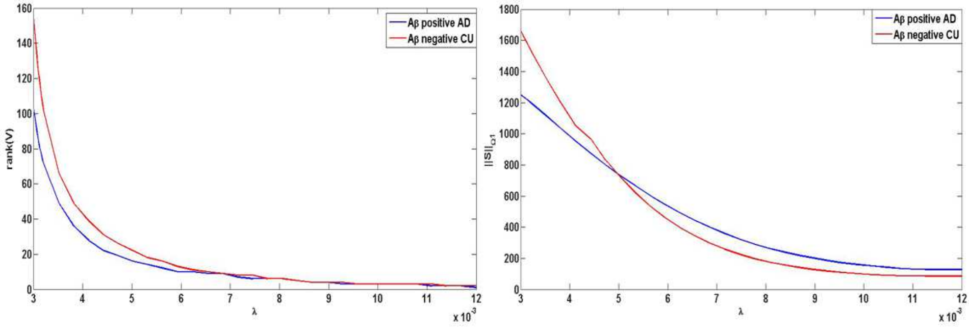
In Eq. 4, we see that the parameter which controls the relative importance of the low-rank term vs. the sparse term was set as , where and represent the numbers of rows and columns in the observation data matrix. To understand the relationships between the , with the different values of the parameter , we chose the AD and CU group as the research objects. We find that the and tend to decrease with an increase of the , as shown in Fig. 6. Because the threshold of the sparse component constraint is increasing with the increase of the in the Eq. 9, the immediate result is the decrease of the . In addition, although the change of is not directly related to the change of , results indicate that the decrease due to gradually increasing removal of the noise and the sparse term with the increase of . And the is stable when was greater than 0.006. However, when the become too large, it results in homogeneous structures, reducing the discriminatory power for classifying the AD and CU groups. To validate the distinguishing power of the UMIs generated under different , we randomly use 90 of the AD and CU group as the training data to extract the common structures of these two groups with each . The generated UMIs from remaining 10 of these two groups are classified using ROC analysis. This process is repeated 10 times. The average classification error rates with the different are shown in Table 7. The results show that both high or low will lead to an increase in classification error rate. This indicates that a low introduces excessive noise and residual information of individuals and a high makes the common structures of the two groups tend to be consistent. In both cases, the generated ROI cannot correctly reflect the morphological changes caused by AD, resulting in a decrease in UMI classification results. Based on the above discussion, is empirically set as throughout this paper.
| UMI-AD | UMI-CU | classification error | |
|---|---|---|---|
| 0.003 | |||
| 0.004 | |||
| 0.005 | |||
| 0.006 | |||
| 0.007 | |||
| 0.008 | |||
| 0.009 | |||
| 0.01 | |||
| 0.011 | |||
| 0.012 | |||
| 0.013 | |||
| 0.014 |
4.2 Effect Size Comparison Between A and A subjects in the Longitudinal Study
To further validate the subspace decomposition-based UMIs have strong discrimination power for detecting the morphological changes induced by ADD, we analyze additional longitudinal A subjects from ADNI database comparable to the A group, which includes AD, MCI and CTL subjects. The demographic characteristic statistics information and the obtained UMIs for these samples are shown in Table 8. Similar to A data, after the registration, surface deformation statistics are computed to obtain the raw RDs of all the longitudinal A subjects. Based on the predefined ROIs (Fig. 2 (a) and (c) in Section 3.1) and the AD atrophy degrees, we compute the UMIs of different longitudinal A groups.
| Gender(M/F) | Education | Age | MMSE | UMI | |
|---|---|---|---|---|---|
| AD baseline | |||||
| AD m24 | |||||
| MCI baseline | |||||
| MCI m24 | |||||
| CU baseline | |||||
| CU m24 |
| UMIs | Volume Measures | |
|---|---|---|
| AD | ||
| MCI | ||
| CTL |
Then we use Cohen’s d as effect size measure to test the differences between the univariate biomarkers (UMI vs. volume measure) changes of the longitudinal A group and those of A group in same clinical groups (AD, MCI and CU). The effect size comparison results are shown in Table 9. The results show that the differences between UMI changes of the longitudinal A group and those of the longitudinal A group are more significant than the differences between volume changes of the longitudinal A group and those of the longitudinal A group. Since the UMIs are defined on the ROIs induced by ADD, it leads to larger changes in UMIs of longitudinal A group, and smaller changes in UMIs of longitudinal A group. The results may also justify that the subspace decomposition-based UMIs have strong discrimination power for detecting the morphological changes induced by ADD.
| Group | variables | R | CI of R | -value of R |
|---|---|---|---|---|
| AD | UMI vs. CDR-SB | |||
| UMI vs. ADAS-Cog11 | ||||
| UMI vs. MMSE | ||||
| MCI | UMI vs. CDR-SB | |||
| UMI vs. ADAS-Cog11 | ||||
| UMI vs. MMSE | ||||
| CU | UMI vs. CDR-SB | |||
| UMI vs. ADAS-Cog11 | ||||
| UMI vs. MMSE |
4.3 Correlation Analysis with Cognitive Outcomes in Different Clinical Groups
In this section, we investigate whether changes of UMI results are correlated with changes of clinical rating scores within 24 months, such as Clinical Dementia Rating Sum of Boxes CDR-SB (Morris 1993), AD Assessment Scale-Cognitive Subscale (ADAS-Cog11) (Rosen et al. 1984) and MMSE scores. CDR-SB, ADAS-Cog11 scores are used to help track the progression of cognitive impairment, where a higher score indicates more severe dementia. Here we use the same longitudinal subjects ( AD, MCI and CU in Section 3.2) and with the Pearson parametric test (Lemasson et al. 2012), we explore the correlation between the UMI changes and the clinical outcome changes within 24 months, including CDR-SB, ADAS-Cog11 and MMSE scores. The correlation analysis results, i.e., correlation coefficients (R), confidential intervals of R and correlation significance of -test for R between the UMI changes and the changes of CDR-SB, ADAS-Cog11 and MMSE scores for different longitudinal groups are shown in Table 10.
Results show that the UMIs of longitudinal AD and MCI groups have moderate correlations with the CDR-SB, ADAS-Cog11 and MMSE scores. This is likely due to that the proposed UMIs well correlate with clinical outcomes within longitudinal AD and MCI groups. However, the correlations between the UMIs and the CDR-SB and MMSE scores of longitudinal CU group are not so significant as that of AD and MCI groups. From the perspective of data distribution, it is due to the fact that the distribution trend of the morphological changes depicted by UMIs differs from the distribution trend of the cognitive changes depicted by CDR-SB and MMSE scores within longitudinal CU group. A plausible reason may be that the morphological changes caused by AD occurred before the cognitive decline in the stage of unimpaired cognition, as proposed in the hypothetical model of AD biomarkers (Jack et al. 2013) and validated in a number of prior work (Sperling et al. 2011; Jack et al. 2018; Weston et al. 2016; Zhao et al. 2017), including our own study (Dong et al. 2019).

4.4 Assessment of Enrichment Performance
To evaluate the enrichment performance of UMIs, we use a cut-point based enrichment strategy (Yu et al. 2014) in longitudinal MCI group (the same MCI group in Section 3.2 denoted as unenriched group) to select the MCI subgroup (enriched group) and calculate the three clinical characteristics (CDR-SB, MMSE and ADAS-Cog11) of the selected MCI subgroup. The enrichment strategy is implemented as follows. First, a range of cutoff values are determined as the , and percentiles of UMIs in the CU cohort ( CU subjects in Section 3.1), which serve as a normative reference population. Secondly, for each cutoff value, we extract the clinical characteristics of the selected MCI subgroup and derive implications for clinical trials where only this subgroup will be enrolled. We calculate the effect size of the 24-months change in each of the three clinical measures. Denoting the effect size of the enriched group by and the unenriched group by , we then calculate the sample size required to achieve a statistical power equivalent to an unenriched group of size (Yu et al. 2014). The comparison results of effect sizes and sample sizes of different clinical measures for the specific cut-points, i.e., , and percentiles of the UMIs distribution of CU cohort, are shown in Fig. 7.
In the upper plot of Fig. 7, the results show that the effect sizes of all three clinical measures increase in all enriched group according to the specific cutoff values, comparing to the unenriched group. In general, more stringent cutoff values (higher UMI thresholds) lead to greater effect size. Cut-points corresponding to the , and percentiles of the CU cohort distribution yield effect sizes of (CDR-SB), (ADAS-Cog11) and (MMSE) greater than the unenriched group. The sample size results are shown in the lower plot of Fig. 7. Reduced sample sizes are obtained across the three cut-points for the three clinical measures. Error bars indicate confidence intervals of the estimated sample sizes. For cut-points corresponding to , and percentiles of the UMIs distribution of CU cohort, sample sizes corresponding to (CDR-SB), (ADAS-Cog11) and (MMSE) of the unenriched case () are estimated. This indicates that subspace decomposition-based UMIs provides an enrichment biomarker to select a fraction of the screening group that is likely to imminently progress most rapidly.
4.5 Comparison with Heat Kernel Smoothing
The motivation of our subspace decomposition work is to increase the signal-to-noise (SNR) and improve the sensitivity of statistical analysis. Surface smoothing work, especially heat kernel smoothing algorithm (Chung et al. 2005), has been adopted in our prior work (Shi et al. 2015; Paquette et al. 2017, e.g.) to increase the SNR of surface tensor-based morphometry (TBM) features and boost the sensitivity of statistical analysis. Here we use the heat kernel smoothing results to generate UMIs and compare its performance with the one of our subspace decomposition-based UMIs. First, we use heat kernel smoothing (the kernel width=1 and the number of iteration=100) to generate the smoothed hippocampal RD measures of the same subjects in Section 3.1, i.e., AD patients and CU subjects. Second, following the content of Section 3.1, we randomly select of the subjects in each group to generate ROIs. This process is repeated 10 times. At each time, the regions of significant smoothed RD difference (ROIs) between AD group and CU group are assessed via the two-sample -test with random field theory based -value correction. Here, we use -value correction method (Benjamini and Hochberg 1995) to controlling the false discovery rate (FDR). The desired false discovery rate () is set as and the generated ROIs are the vertices whose -test corrected -values represent the group differences smaller than . The results of the generated ROIs are shown in Fig. 8. Non-blue colors indicate the number of times a vertex is selected. The red color denotes that the vertex is selected for 10 times after 10 ROI generation processes. From the results, we can see that the selected ROIs based on the smoothed RD measures have a certain degree of similarity with the ROIs based on low-rank components. This indicated that heat kernel smoothing and subspace decomposition have similar effects in improving the stability of the ROI generation.

Using AD atrophy degrees and individual atrophy degrees on the generated ROIs based on the smoothed RD measures, we compute the UMIs of the longitudinal subjects according to the Eq. 14. With Eq. 15, we estimate the minimum sample sizes of UMIs based on the smoothed RD measures. The minimum sample sizes of the longitudinal AD, MCI and CU groups are 261, 374 and 546, respectively. The results show that the minimum sample sizes from the UMIs based on smoothed RD measures are all smaller than those based on raw RD measures. This indicates that heat kernel smoothing may increase the SNR and the sensitivity of statistical analysis. On the other hand, the results show that the minimum sample sizes from the heat kernel smoothing-based UMIs are all larger than low-rank decomposition-based UMIs, indicating that the low-rank decomposition-based UMIs gain more statistical power than those of the heat kernel smoothing-based UMIs. Part of the reason may be due to the fact that the decomposed low rank and subspace better characterizes group level morphometry features.
4.6 Limitations
The proposed low-rank and sparse subspace decomposition-based UMI represents our initial efforts to develop robust ROI-based UNB. Nonetheless, there are several limitations of this study to consider. First, a relatively small number of subjects are included as the research objects, e.g. the ROIs are extracted from AD patients and CU subjects, which are certainly not enough to fully characterize the general morphological change patterns caused by ADD. Consequently, the range of morphological characteristics of individuals identified by the computed UMIs are likely incomplete. Besides, we have not tested our UMI framework together with the discovered ROIs in a cohort other than ADNI. Even so, our current results demonstrate the proposed approach may improve statistical power in a variety of UNB applications. Effect size comparison results also show that this proposed UMI measure is more sensitive to detect the hippocampal morphological changes than hippocampal volume measure. Second, we choose the RD as the hippocampal morphological feature because RD has been applied in several subcortical studies and served as an ideal description of the hippocampal structural changes induced by ADD. However, tensor-based morphometry (Chung et al. 2008) and multivariate TBM (Wang et al. 2011) may be sensitive to deformations such as rotation, dilation, and shear along the surface tangent direction, and theorefore the TBM or mTBM may effectively capture hippocampal structural alterations (e.g. atrophy and enlargement) in tensor fields. The ability to describe the morphological features of the hippocampus will be enhanced if we combine the TBM or mTBM measures and the RD measure. Third, in this study, we are using UMIs alone to predict rates of progression from MCI to probable AD without combining other types of biomarkers, such as amyloid/tau/neurodegeneration (A/T/N) measurement framework (Jack et al. 2016), fluorodeoxyglucose positron emission tomography (FDG-PET) measurements of the regional cerebral metabolic rate for glucose (CMRgl) decline (Landau et al. 2010) as a marker of clinical AD progression, fibrillar amyloid- PET measurements using Pittsburgh Compound B (PiB) (Ikonomovic et al. 2008) and cerebrospinal fluid (CSF) amyloid levels (Fagan et al. 2007) as biomarkers of AD pathology. If we combine these biomarkers with UMIs and carry out multivariate Cox analyses, the correctness of survival probabilities would likely be improved.
5 Conclusion
In this paper, we present a univariate neurodegeneration biomarker generation framework based on subspace decomposition to correctly and effectively depict the morphological changes induced by ADD. Applying the matrix decomposition and the local sparse constraints on the RD observation matrices, we obtain the ROIs closely associated with ADD which are robust to image noise. We then generate the UMIs to improve the statistical power for in vivo MRI morphological analyses. Our empirical results demonstrate the potential that the UMIs may capture the ADD-induced brain morphometry abnormalities of the longitudinal groups at high risk for AD. Based on the optimal classification criterion, the UMIs have strong discrimination power for predicting the conversion rates from MCI subjects (converter and non-converter) to AD. The proposed framework is general and may be generalized to process other 3D brain imaging data, such as PET imaging data (Chen et al. 2011). In future studies, we will also evaluate our method in other brain imaging cohorts, such as Arizona APOE cohort (Caselli et al. 2004; Caselli et al. 2009) and OASIS cohort (LaMontagne et al. 2019).
6 Acknowledgement
This work was partially supported by National Natural Science Foundation of China (61772253, 61771231, 61873117, 61872170, 61903172); NSFC Joint Fund with Zhejiang Integration of Informatization and Industrialization under Key Project (U1609218); Key Research and Development Program of Shandong Province (2019JZZY010125); Shandong Province Higher Educational Science and Technology Program (J17KA050); National Institute on Aging (RF1AG051710, R21AG065942, R01AG031581, P30AG19610); National Institute of Biomedical Imaging and Bioengineering (R01EB025032); and Arizona Alzheimer’s Consortium.
Data collection and sharing for this project was funded by the Alzheimer’s Disease Neuroimaging Initiative (ADNI) (National Institutes of Health Grant U01 AG024904) and DOD ADNI (Department of Defense award number W81XWH-12-2-0012). ADNI is funded by the National Institute on Aging, the National Institute of Biomedical Imaging and Bioengineering, and through generous contributions from the following: Alzheimer’s Association; Alzheimer’s Drug Discovery Foundation; Araclon Biotech; BioClinica, Inc.; Biogen Idec Inc.; Bristol-Myers Squibb Company; Eisai Inc.; Elan Pharmaceuticals, Inc.; Eli Lilly and Company; EuroImmun; F. Hoffmann-La Roche Ltd and its affiliated company Genentech, Inc.; Fujirebio; GE Healthcare; IXICO Ltd.; Janssen Alzheimer Immunotherapy Research & Development, LLC.; Johnson & Johnson Pharmaceutical Research & Development LLC.; Medpace, Inc.; Merck & Co., Inc.; Meso Scale Diagnostics, LLC.; NeuroRx Research; Neurotrack Technologies; Novartis Pharmaceuticals Corporation; Pfizer Inc.; Piramal Imaging; Servier; Synarc Inc.; and Takeda Pharmaceutical Company. The Canadian Institutes of Rev December 5, 2013 Health Research is providing funds to support ADNI clinical sites in Canada. Private sector contributions are facilitated by the Foundation for the National Institutes of Health (www.fnih.org). The grantee organization is the Northern California Institute for Research and Education, and the study is coordinated by the Alzheimer’s Disease Cooperative Study at the University of California, San Diego. ADNI data are disseminated by the Laboratory for Neuro Imaging at the University of Southern California.
References
- Apostolova et al. (2010) Apostolova, L.G., Mosconi, L., Thompson, P.M., Green, A.E., Hwang, K.S., Ramirez, A., Mistur, R., Tsui, W.H., de Leon, M.J., 2010. Subregional hippocampal atrophy predicts Alzheimer’s dementia in the cognitively normal. Neurobiol. Aging 31, 1077–1088.
- Beckett et al. (2010) Beckett, L.A., Harvey, D.J., Gamst, A., Donohue, M., Kornak, J., Zhang, H., Kuo, J.H., 2010. The Alzheimer’s Disease Neuroimaging Initiative: Annual change in biomarkers and clinical outcomes. Alzheimers Dement 6, 257–264.
- Benjamini and Hochberg (1995) Benjamini, Y., Hochberg, Y., 1995. Controlling the False Discovery Rate: A Practical and Powerful Approach to Multiple Testing. Journal of the Royal Statistical Society. Series B (Methodological) 57, 289–300.
- Cai et al. (2008) Cai, J.F., Candès, E.J., Shen, Z., 2008. A singular value thresholding algorithm for matrix completion. Siam Journal on Optimization 20, 1956–1982.
- Candès et al. (2011) Candès, E., Li, X., Ma, Y., Wright, J., 2011. Robust principal component analysis? Journal of ACM 58.
- Cao et al. (2017) Cao, F., Chen, J., Ye, H., Zhao, J., Zhou, Z., 2017. Recovering low-rank and sparse matrix based on the truncated nuclear norm. Neural Networks 85, 10–20.
- Cardenas et al. (2011) Cardenas, V.A., Chao, L.L., Studholme, C., Yaffe, K., Miller, B.L., Madison, C., Buckley, S.T., Mungas, D., Schuff, N., Weiner, M.W., 2011. Brain atrophy associated with baseline and longitudinal measures of cognition. Neurobiol. Aging 32, 572–580.
- Caselli et al. (2009) Caselli, R.J., Dueck, A.C., Osborne, D., Sabbagh, M.N., Connor, D.J., Ahern, G.L., Baxter, L.C., Rapcsak, S.Z., Shi, J., Woodruff, B.K., Locke, D.E., Snyder, C.H., Alexander, G.E., Rademakers, R., Reiman, E.M., 2009. Longitudinal modeling of age-related memory decline and the APOE epsilon4 effect. N. Engl. J. Med. 361, 255–263.
- Caselli and Reiman (2013) Caselli, R.J., Reiman, E.M., 2013. Characterizing the preclinical stages of Alzheimer’s disease and the prospect of presymptomatic intervention. J. Alzheimers Dis. 33 Suppl 1, S405–416.
- Caselli et al. (2004) Caselli, R.J., Reiman, E.M., Osborne, D., Hentz, J.G., Baxter, L.C., Hernandez, J.L., Alexander, G.G., 2004. Longitudinal changes in cognition and behavior in asymptomatic carriers of the APOE e4 allele. Neurology 62, 1990–1995.
- Chen et al. (2011) Chen, K., Ayutyanont, N., Langbaum, J.B., Fleisher, A.S., Reschke, C., Lee, W., Liu, X., Bandy, D., Alexander, G.E., Thompson, P.M., Shaw, L., Trojanowski, J.Q., Jack, C.R., Landau, S.M., Foster, N.L., Harvey, D.J., Weiner, M.W., Koeppe, R.A., Jagust, W.J., Reiman, E.M., 2011. Characterizing Alzheimer’s disease using a hypometabolic convergence index. Neuroimage 56, 52–60.
- Chen et al. (2007) Chen, K., Reiman, E.M., Alexander, G.E., Caselli, R.J., Gerkin, R., Bandy, D., Domb, A., Osborne, D., Fox, N., Crum, W.R., Saunders, A.M., Hardy, J., 2007. Correlations between apolipoprotein E epsilon4 gene dose and whole brain atrophy rates. Am J Psychiatry 164, 916–921.
- Chung et al. (2008) Chung, M.K., Dalton, K.M., Davidson, R.J., 2008. Tensor-based cortical surface morphometry via weighted spherical harmonic representation. IEEE Trans Med Imaging 27, 1143–1151.
- Chung et al. (2005) Chung, M.K., Robbins, S.M., Dalton, K.M., Davidson, R.J., Alexander, A.L., Evans, A.C., 2005. Cortical thickness analysis in autism with heat kernel smoothing. NeuroImage 25, 1256 – 1265.
- Chupin et al. (2009) Chupin, M., Gerardin, E., Cuingnet, R., Boutet, C., Lemieux, L., Lehericy, S., Benali, H., Garnero, L., Colliot, O., 2009. Fully automatic hippocampus segmentation and classification in Alzheimer’s disease and mild cognitive impairment applied on data from ADNI. Hippocampus 19, 579–587.
- Chupin et al. (2007) Chupin, M., Mukuna-Bantumbakulu, A.R., Hasboun, D., Bardinet, E., Baillet, S., Kinkingn?hun, S., Lemieux, L., Dubois, B., Garnero, L., 2007. Anatomically constrained region deformation for the automated segmentation of the hippocampus and the amygdala: Method and validation on controls and patients with Alzheimer’s disease. Neuroimage 34, 996–1019.
- Cortechs Labs (2020) Cortechs Labs, 2020. NeuroQuant. https://www.cortechslabs.com/products/neuroquant.
- Costafreda et al. (2011) Costafreda, S.G., Dinov, I.D., Tu, Z., Shi, Y., Liu, C.Y., Kloszewska, I., Mecocci, P., Soininen, H., Tsolaki, M., Vellas, B., Wahlund, L.O., Spenger, C., Toga, A.W., Lovestone, S., Simmons, A., 2011. Automated hippocampal shape analysis predicts the onset of dementia in mild cognitive impairment. Neuroimage 56, 212–219.
- Crivello et al. (2014) Crivello, P., Zito, L., Sizzano, F., Zino, E., Maiers, M., Mulder, A., Toffalori, C., Naldini, L., Ciceri, F., Vago, L., Fleischhauer, K., 2014. The impact of amino acid variability defines a functional distance predictive of permissive hla-dpb1 mismatches in hematopoietic cell transplantation. Biology of blood and marrow transplantation : journal of the American Society for Blood and Marrow Transplantation 21.
- Dickerson et al. (2009) Dickerson, B.C., Bakkour, A., Salat, D.H., Feczko, E., Pacheco, J., Greve, D.N., Grodstein, F., Wright, C.I., Blacker, D., Rosas, H.D., Sperling, R.A., Atri, A., Growdon, J.H., Hyman, B.T., Morris, J.C., Fischl, B., Buckner, R.L., 2009. The cortical signature of Alzheimer’s disease: regionally specific cortical thinning relates to symptom severity in very mild to mild AD dementia and is detectable in asymptomatic amyloid-positive individuals. Cereb. Cortex 19, 497–510.
- Dong et al. (2020) Dong, Q., Zhang, W., Stonnington, C.M., Wu, J., Gutman, B.A., Chen, K., Su, Y., Baxter, L.C., Thompson, P.M., Reiman, E.M., Caselli, R.J., Wang, Y., 2020. Applying surface-based morphometry to study ventricular abnormalities of cognitively unimpaired subjects prior to clinically significant memory decline. Neuroimage Clin 27, 102338.
- Dong et al. (2019) Dong, Q., Zhang, W., Wu, J., Li, B., Schron, E.H., McMahon, T., Shi, J., Gutman, B.A., Chen, K., Baxter, L.C., Thompson, P.M., Reiman, E.M., Caselli, R.J., Wang, Y., 2019. Applying surface-based hippocampal morphometry to study APOE-E4 allele dose effects in cognitively unimpaired subjects. Neuroimage Clin 22, 101744.
- Douglas and Rachford (1956) Douglas, J., Rachford, H.H., 1956. On the numerical solution of the heat conduction problem in 2 and 3 space variables. Transactions of the American Mathematical Society 82, 421–439.
- Fagan et al. (2007) Fagan, A.M., Roe, C.M., Xiong, C., Mintun, M.A., Morris, J.C., Holtzman, D.M., 2007. Cerebrospinal fluid tau/beta-amyloid(42) ratio as a prediction of cognitive decline in nondemented older adults. Arch. Neurol. 64, 343–349.
- Folstein et al. (1975) Folstein, M.F., Folstein, S.E., McHugh, P.R., 1975. "Mini-mental state". A practical method for grading the cognitive state of patients for the clinician. J Psychiatr Res 12, 189–198.
- Fox et al. (1999) Fox, N.C., Scahill, R.I., Crum, W.R., Rossor, M.N., 1999. Correlation between rates of brain atrophy and cognitive decline in AD. Neurology 52, 1687–1689.
- Frisoni et al. (2010) Frisoni, G.B., Fox, N.C., Jack, C.R., Scheltens, P., Thompson, P.M., 2010. The clinical use of structural MRI in Alzheimer disease. Nat Rev Neurol 6, 67–77.
- Gill (2007) Gill, P.M.W., 2007. Efficient calculation of p-values in linear-statistic permutation significance tests. Journal of Statistical Computation and Simulation 77, 55–61.
- Gutman et al. (2013) Gutman, B.A., Hua, X., Rajagopalan, P., Chou, Y.Y., Wang, Y., Yanovsky, I., Toga, A.W., Jack, C.R., Weiner, M.W., Thompson, P.M., 2013. Maximizing power to track Alzheimer’s disease and MCI progression by LDA-based weighting of longitudinal ventricular surface features. Neuroimage 70, 386–401.
- Han et al. (2003) Han, X., Xu, C., Prince, J., 2003. A topology preserving level set method for geometric deformable models. IEEE Transactions on Pattern Analysis and Machine Intelligence 25, 755–768.
- Hastie et al. (2015) Hastie, T., Tibshirani, R., Wainwright, M., 2015. Statistical Learning with Sparsity: The Lasso and Generalizations. Chapman and Hall/CRC.
- den Heijer et al. (2010) den Heijer, T., van der Lijn, F., Koudstaal, P.J., Hofman, A., van der Lugt, A., Krestin, G.P., Niessen, W.J., Breteler, M.M., 2010. A 10-year follow-up of hippocampal volume on magnetic resonance imaging in early dementia and cognitive decline. Brain 133, 1163–1172.
- Higham and Papadimitriou (1995) Higham, N., Papadimitriou, P., 1995. Matrix procrustes problems. Rapport technique, University of Manchester .
- Hoppe (1996) Hoppe, H., 1996. Progressive meshes, in: Proceedings of the 23rd Annual Conference on Computer Graphics and Interactive Techniques, Association for Computing Machinery, New York, NY, USA. p. 99–108.
- Hosmer et al. (2008) Hosmer, D.W., Lemeshow, S., May, S., 2008. Applied Survival Analysis: Regression Modeling of Time-to-Event Data. Wiley-Interscience.
- Hua et al. (2011) Hua, X., Gutman, B., Boyle, C.P., Rajagopalan, P., Leow, A.D., Yanovsky, I., Kumar, A.R., Toga, A.W., Jack, C.R., Schuff, N., Alexander, G.E., Chen, K., Reiman, E.M., Weiner, M.W., Thompson, P.M., 2011. Accurate measurement of brain changes in longitudinal MRI scans using tensor-based morphometry. Neuroimage 57, 5–14.
- Hua et al. (2010) Hua, X., Lee, S., Hibar, D.P., Yanovsky, I., Leow, A.D., Toga, A.W., Jack, C.R., Bernstein, M.A., Reiman, E.M., Harvey, D.J., Kornak, J., Schuff, N., Alexander, G.E., Weiner, M.W., Thompson, P.M., 2010. Mapping Alzheimer’s disease progression in 1309 MRI scans: power estimates for different inter-scan intervals. Neuroimage 51, 63–75.
- Ikonomovic et al. (2008) Ikonomovic, M.D., Klunk, W.E., Abrahamson, E.E., Mathis, C.A., Price, J.C., Tsopelas, N.D., Lopresti, B.J., Ziolko, S., Bi, W., Paljug, W.R., Debnath, M.L., Hope, C.E., Isanski, B.A., Hamilton, R.L., DeKosky, S.T., 2008. Post-mortem correlates of in vivo PiB-PET amyloid imaging in a typical case of Alzheimer’s disease. Brain 131, 1630–1645.
- Illan-Gala et al. (2018) Illan-Gala, I., Pegueroles, J., Montal, V., Vilaplana, E., Carmona-Iragui, M., Alcolea, D., Dickerson, B.C., Sanchez-Valle, R., de Leon, M.J., Blesa, R., Llea, A., Fortea, J., 2018. Challenges associated with biomarker-based classification systems for Alzheimer’s disease. Alzheimers Dement (Amst) 10, 346–357.
- Jack et al. (1999) Jack, C., Petersen, R., Xu, Y., O’Brien, P., Smith, G., Ivnik, R., Boeve, B., Waring, S., Tangalos, E., Kokmen, E., 1999. Prediction of ad with mri-based hippocampal volume in mild cognitive impairment. Neurology 52, 1397–1397.
- Jack et al. (2018) Jack, C.R., Bennett, D.A., Blennow, K., Carrillo, M.C., Dunn, B., Haeberlein, S.B., Holtzman, D.M., Jagust, W., Jessen, F., Karlawish, J., Liu, E., Molinuevo, J.L., Montine, T., Phelps, C., Rankin, K.P., Rowe, C.C., Scheltens, P., Siemers, E., Snyder, H.M., Sperling, R., Elliott, C., Masliah, E., Ryan, L., Silverberg, N., 2018. NIA-AA Research Framework: Toward a biological definition of Alzheimer’s disease. Alzheimers Dement 14, 535–562.
- Jack et al. (2016) Jack, C.R., Bennett, D.A., Blennow, K., Carrillo, M.C., Feldman, H.H., Frisoni, G.B., Hampel, H., Jagust, W.J., Johnson, K.A., Knopman, D.S., Petersen, R.C., Scheltens, P., Sperling, R.A., Dubois, B., 2016. A/T/N: An unbiased descriptive classification scheme for Alzheimer disease biomarkers. Neurology 87, 539–547.
- Jack et al. (2013) Jack, C.R., Knopman, D.S., Jagust, W.J., Petersen, R.C., Weiner, M.W., Aisen, P.S., Shaw, L.M., Vemuri, P., Wiste, H.J., Weigand, S.D., Lesnick, T.G., Pankratz, V.S., Donohue, M.C., Trojanowski, J.Q., 2013. Tracking pathophysiological processes in Alzheimer’s disease: an updated hypothetical model of dynamic biomarkers. Lancet Neurol 12, 207–216.
- Jack et al. (2003) Jack, C.R., Slomkowski, M., Gracon, S., Hoover, T.M., Felmlee, J.P., Stewart, K., Xu, Y., Shiung, M., O’Brien, P.C., Cha, R., Knopman, D., Petersen, R.C., 2003. MRI as a biomarker of disease progression in a therapeutic trial of milameline for AD. Neurology 60, 253–260.
- Jang et al. (2016) Jang, W.D., Lee, C., Kim, C.S., 2016. Primary object segmentation in videos via alternate convex optimization of foreground and background distributions, in: Proceedings of the IEEE conference on computer vision and pattern recognition, pp. 696–704.
- Javed et al. (2016) Javed, S., Mahmood, A., Bouwmans, T., Jung, S., 2016. Spatiotemporal low-rank modeling for complexscene background initialization. IEEE Transactions on Circuits and Systems for Video Technology 28, 1315–1329.
- Knopman et al. (2018) Knopman, D.S., Haeberlein, S.B., Carrillo, M.C., Hendrix, J.A., Kerchner, G., Margolin, R., Maruff, P., Miller, D.S., Tong, G., Tome, M.B., Murray, M.E., Nelson, P.T., Sano, M., Mattsson, N., Sultzer, D.L., Montine, T.J., Jack, C.R., Kolb, H., Petersen, R.C., Vemuri, P., Canniere, M.Z., Schneider, J.A., Resnick, S.M., Romano, G., van Harten, A.C., Wolk, D.A., Bain, L.J., Siemers, E., 2018. The National Institute on Aging and the Alzheimer’s Association Research Framework for Alzheimer’s disease: Perspectives from the Research Roundtable. Alzheimers Dement 14, 563–575.
- LaMontagne et al. (2019) LaMontagne, P.J., Benzinger, T.L., Morris, J.C., Keefe, S., Hornbeck, R., Xiong, C., Grant, E., Hassenstab, J., Moulder, K., Vlassenko, A., Raichle, M.E., Cruchaga, C., Marcus, D., 2019. Oasis-3: Longitudinal neuroimaging, clinical, and cognitive dataset for normal aging and alzheimer disease. medRxiv https://www.medrxiv.org/content/early/2019/12/15/2019.12.13.19014902.full.pdf.
- Landau et al. (2010) Landau, S.M., Harvey, D., Madison, C.M., Reiman, E.M., Foster, N.L., Aisen, P.S., Petersen, R.C., Shaw, L.M., Trojanowski, J.Q., Jack, C.R., Weiner, M.W., Jagust, W.J., 2010. Comparing predictors of conversion and decline in mild cognitive impairment. Neurology 75, 230–238.
- Langbaum et al. (2013) Langbaum, J.B., Fleisher, A.S., Chen, K., Ayutyanont, N., Lopera, F., Quiroz, Y.T., Caselli, R.J., Tariot, P.N., Reiman, E.M., 2013. Ushering in the study and treatment of preclinical Alzheimer disease. Nat Rev Neurol 9, 371–381.
- Lemasson et al. (2012) Lemasson, B., Christen, T., Serduc, R., Maisin, C., Bouchet, A., Le Duc, G., Remy, C., Barbier, E.L., 2012. Evaluation of the relationship between MR estimates of blood oxygen saturation and hypoxia: effect of an antiangiogenic treatment on a gliosarcoma model. Radiology 265, 743–752.
- Lin et al. (2009) Lin, Z., Chen, M., Wu, L., Ma, Y., 2009. The augmented lagrange multiplier method for exact recovery of corrupted low-rank matrices. Coordinated Science Laboratory Report no. UILU-ENG-09-2215, DC-247 .
- Lin and Zhang (2017) Lin, Z., Zhang, H., 2017. Low-Rank Models in Visual Analysis: Theories, Algorithms, and Applications. Academic Press, Inc., USA. 1st edition.
- Liu and Yan (2012) Liu, G., Yan, S., 2012. Active subspace: Toward scalable low-rank learning. Neural Computation 24, 427–444.
- Loop (1987) Loop, C., 1987. Smooth Subdivision Surfaces Based on Triangles. Master’s thesis. The University of Utah.
- Lorensen and Cline (1987) Lorensen, W.E., Cline, H.E., 1987. Marching cubes: A high resolution 3D surface construction algorithm, in: Proceedings of the 14th Annual Conference on Computer Graphics and Interactive Techniques, Association for Computing Machinery, New York, NY, USA. p. 163–169.
- Morris (1993) Morris, J.C., 1993. The Clinical Dementia Rating (CDR): current version and scoring rules. Neurology 43, 2412–2414.
- Mueller et al. (2005) Mueller, S.G., Weiner, M.W., Thal, L.J., Petersen, R.C., Jack, C., Jagust, W., Trojanowski, J.Q., Toga, A.W., Beckett, L., 2005. The Alzheimer’s disease neuroimaging initiative. Neuroimaging Clin. N. Am. 15, 869–877.
- Paquette et al. (2017) Paquette, N., Shi, J., Wang, Y., Lao, Y., Ceschin, R., Nelson, M.D., Panigrahy, A., Lepore, N., 2017. Ventricular shape and relative position abnormalities in preterm neonates. Neuroimage Clin 15, 483–493.
- Patenaude et al. (2011) Patenaude, B., Smith, S., Kennedy, D., Jenkinson, M., 2011. A bayesian model of shape and appearance for subcortical brain segmentation. NeuroImage 56, 907–922.
- Pennanen et al. (2004) Pennanen, C., Kivipelto, M., Tuomainen, S., Hartikainen, P., H?nninen, T., Laakso, M.P., Hallikainen, M., Vanhanen, M., Nissinen, A., Helkala, E.L., Vainio, P., Vanninen, R., Partanen, K., Soininen, H., 2004. Hippocampus and entorhinal cortex in mild cognitive impairment and early AD. Neurobiol. Aging 25, 303–310.
- Pizer et al. (1999) Pizer, S.M., Fritsch, D.S., Yushkevich, P.A., Johnson, V.E., Chaney, E.L., 1999. Segmentation, registration, and measurement of shape variation via image object shape. IEEE Trans Med Imaging 18, 851–865.
- Qiu et al. (2010) Qiu, A., Brown, T., Fischl, B., Ma, J., Miller, M.I., 2010. Atlas generation for subcortical and ventricular structures with its applications in shape analysis. IEEE Trans Image Process 19, 1539–1547.
- Racine et al. (2018) Racine, A.M., Brickhouse, M., Wolk, D.A., Dickerson, B.C., 2018. The personalized Alzheimer’s disease cortical thickness index predicts likely pathology and clinical progression in mild cognitive impairment. Alzheimers Dement (Amst) 10, 301–310.
- Rey (1964) Rey, A., 1964. L’examen clinique en psychologie. Presses Universitaires de France, Paris.
- Rosen et al. (1984) Rosen, W., Mohs, R., Davis, K., 1984. A new rating scale for alzheimer’s disease. American Journal of Psychiatry 141, 1356–1364.
- Sabuncu et al. (2016) Sabuncu, M.R., Ge, T., Holmes, A.J., Smoller, J.W., Buckner, R.L., Fischl, B., 2016. Morphometricity as a measure of the neuroanatomical signature of a trait. Proc. Natl. Acad. Sci. U.S.A. 113, E5749–5756.
- Shi et al. (2015) Shi, J., Stonnington, C.M., Thompson, P.M., Chen, K., Gutman, B., Reschke, C., Baxter, L.C., Reiman, E.M., Caselli, R.J., Wang, Y., 2015. Studying ventricular abnormalities in mild cognitive impairment with hyperbolic Ricci flow and tensor-based morphometry. Neuroimage 104, 1–20.
- Shi et al. (2013) Shi, J., Thompson, P.M., Gutman, B., Wang, Y., 2013. Surface fluid registration of conformal representation: application to detect disease burden and genetic influence on hippocampus. Neuroimage 78, 111–134.
- Sperling et al. (2011) Sperling, R.A., Aisen, P.S., Beckett, L.A., Bennett, D.A., Craft, S., Fagan, A.M., Iwatsubo, T., Jack, C.R., Kaye, J., Montine, T.J., Park, D.C., Reiman, E.M., Rowe, C.C., Siemers, E., Stern, Y., Yaffe, K., Carrillo, M.C., Thies, B., Morrison-Bogorad, M., Wagster, M.V., Phelps, C.H., 2011. Toward defining the preclinical stages of Alzheimer’s disease: recommendations from the National Institute on Aging-Alzheimer’s Association workgroups on diagnostic guidelines for Alzheimer’s disease. Alzheimers Dement 7, 280–292.
- Stonnington et al. (2010) Stonnington, C., Chu, C., Kloppel, S., Jack, C., Ashburner, J., Frackowiak, R., 2010. Predicting clinical scores from magnetic resonance scans in alzheimer’s disease. Neuroimage 51, 1405–13.
- Styner et al. (2006) Styner, M., Oguz, I., Xu, S., Brechbuhler, C., Pantazis, D., Levitt, J.J., Shenton, M.E., Gerig, G., 2006. Framework for the Statistical Shape Analysis of Brain Structures using SPHARM-PDM. Insight J , 242–250.
- Tao and Yuan (2011) Tao, M., Yuan, X., 2011. Recovering low-rank and sparse components of matrices from incomplete and noisy observations. SIAM Journal on Optimization 21, 57–81.
- Thompson et al. (2004) Thompson, P.M., Hayashi, K.M., De Zubicaray, G.I., Janke, A.L., Rose, S.E., Semple, J., Hong, M.S., Herman, D.H., Gravano, D., Doddrell, D.M., Toga, A.W., 2004. Mapping hippocampal and ventricular change in Alzheimer disease. Neuroimage 22, 1754–1766.
- Tseng (2008) Tseng, P., 2008. On accelerated proximal gradient methods for convex-concave optimization. SIAM Journal on Optimization .
- Tu et al. (2020) Tu, Y., Mi, L., Zhang, W., H., Z., Zhang, J., Fan, Y., Goradia, D., Chen, K., Caselli, R.J., Reiman, E.M., Gu, X., Wang, Y., 2020. Computing univariate neurodegenerative biomarkers with volumetric optimal transportation: A pilot study. Neuroinformatics .
- Vemuri et al. (2008) Vemuri, P., Gunter, J.L., Senjem, M.L., Whitwell, J.L., Kantarci, K., Knopman, D.S., Boeve, B.F., Petersen, R.C., Jack, C.R., 2008. Alzheimer’s disease diagnosis in individual subjects using structural MR images: validation studies. Neuroimage 39, 1186–1197.
- Vidal et al. (2016) Vidal, R., Ma, Y., Sastry, S.S., 2016. Generalized Principal Component Analysis. Springer Publishing Company, Incorporated. 1st edition.
- Wang et al. (2012) Wang, H., Nie, F., Huang, H., Yan, J., Kim, S., Nho, K., Risacher, S.L., Saykin, A.J., Shen, L., 2012. From phenotype to genotype: an association study of longitudinal phenotypic markers to Alzheimer’s disease relevant SNPs. Bioinformatics 28, i619–i625.
- Wang et al. (2018) Wang, X., Yan, J., Yao, X., Kim, S., Nho, K., Risacher, S.L., Saykin, A.J., Shen, L., Huang, H., 2018. Longitudinal Genotype-Phenotype Association Study through Temporal Structure Auto-Learning Predictive Model. J. Comput. Biol. 25, 809–824.
- Wang et al. (2011) Wang, Y., Song, Y., Rajagopalan, P., An, T., Liu, K., Chou, Y.Y., Gutman, B., Toga, A.W., Thompson, P.M., 2011. Surface-based TBM boosts power to detect disease effects on the brain: an N=804 ADNI study. Neuroimage 56, 1993–2010.
- Weston et al. (2016) Weston, P.S., Nicholas, J.M., Lehmann, M., Ryan, N.S., Liang, Y., Macpherson, K., Modat, M., Rossor, M.N., Schott, J.M., Ourselin, S., Fox, N.C., 2016. Presymptomatic cortical thinning in familial Alzheimer disease: A longitudinal MRI study. Neurology 87, 2050–2057.
- Yu et al. (2014) Yu, P., Sun, J., Wolz, R., Stephenson, D., Brewer, J., Fox, N.C., Cole, P.E., Jack, C.R., Hill, D.L., Schwarz, A.J., 2014. Operationalizing hippocampal volume as an enrichment biomarker for amnestic mild cognitive impairment trials: effect of algorithm, test-retest variability, and cut point on trial cost, duration, and sample size. Neurobiol. Aging 35, 808–818.
- Zhao et al. (2017) Zhao, Y., Raichle, M.E., Wen, J., Benzinger, T.L., Fagan, A.M., Hassenstab, J., Vlassenko, A.G., Luo, J., Cairns, N.J., Christensen, J.J., Morris, J.C., Yablonskiy, D.A., 2017. In vivo detection of microstructural correlates of brain pathology in preclinical and early Alzheimer Disease with magnetic resonance imaging. Neuroimage 148, 296–304.
- Zhou et al. (2010) Zhou, Z., Li, X., Wright, J., Candes, E., Ma, Y., 2010. Stable principal component pursuit, in: IEEE ISIT Proceedings, ISIT 2010, pp. 1518–1522.