Data-Driven Stabilization of Periodic Orbits

Since their inception by Henri Poincaré at the turn of the twentieth century, return maps, or Poincaré maps as they are now commonly referred, have significantly influenced our understanding of recurrent and chaotic dynamical systems. Poincaré showed that one can understand the dynamics of a system in phase space not by looking at the full trajectory, but by tracking where trajectories intersect a lower-dimensional subspace, transverse to the flow. Such a subspace is now referred to as a Poincaré section, with the mapping that iterates between successive intersections of this section called the Poincaré mapping. Using a Poincaré mapping has the effect that continuous time-dependent behaviour of a dynamical system is translated into a discrete iterative process with a lower-dimensional phase-space. Importantly, fixed points and periodic/cyclic orbits of this mapping manifest themselves as periodic orbits of the continuous-time dynamical system, and therefore Poincaré mappings provide an accessible method of understanding the flow on and near periodic orbits in phase space, many of which are unstable and ultimately responsible for the rich, dynamical structures manifest in many systems. Indeed, as we demonstrate, by exploiting data-driven methods for identifying such unstable periodic orbits, we can then stabilize a system by prescribing appropriate perturbations to its parameters to achieve a desired dynamic outcome.

It is through discrete dynamical systems, such as Poincaré mappings, that much of our modern understanding of chaos comes from as well [1, 2]. Concepts such as horseshoe mappings and symbolic dynamics now inform a significant portion of our comprehension of the geometry of a chaotic attractor. Particularly, it is known that any chaotic attractor contains an infinite number of unstable periodic orbits (UPOs) and that many dynamical averages such as Lyapunov exponents, entropy, and fractal dimensions can be expressed in terms of a weighted sum over the embedded UPOs [3, 4, 5, 2]. UPOs play an important role in our modern understanding of several complex dynamical systems, such as turbulent fluid flow and transport in the solar system. In turbulence, UPOs guide the spatio-temporal chaos observed in spatially-extended fluid models such as the Navier–Stokes equations [6, 7, 8, 9, 10, 11, 12, 13, 14, 15]. There have also been considerable advances in energy efficient space mission design that take advantage of UPOs in the solar system [16, 17, 18].

In their seminal work, Ott, Grebogi, and Yorke demonstrated that these UPOs could be leveraged to control chaotic trajectories through small, precise parameter manipulations at each iterate of the mapping [19]. They proposed that when a chaotic trajectory comes sufficiently close to an element of a desired UPO, well-chosen parameter perturbations could be applied to keep the trajectory close to the chosen UPO, thus stabilizing the unstable orbit. They further commented that the ergodicity of orbits on the chaotic attractor would guarantee that eventually any chaotic trajectory comes sufficiently close to any element of the desired UPO, upon which the control algorithm can then be implemented. Hence, their method constitutes closed-loop control since the action from the controller is dependent on measurements of the system at each iteration.

Since the original work of [19], a number of advances have been made to simplify and extend algorithms for controlling chaos. From these extensions, the control of chaos has been successfully applied to cardiac rhythms [20], mechanical systems [21], synchronizing electrical circuits [22], satellite systems [23], and more. The reviews [24, 25, 26, 27] and the references therein provide an overview of the many advances in this area, as well as a more complete discussion of the applications.

Despite the success of controlling chaos through these methods, there are still significant limitations that must be addressed before they can be applied to a broader range of chaotic systems. Primary among these issues is that of identifying an explicit Poincaré mapping. That is, aside from a few simple examples, there remains the challenge of obtaining an explicit parameter-dependent mapping that governs the iterates of a system inside a Poincaré section – even for many simple dynamical systems. As the numerous studies on chaos control have shown, a closed-form Poincaré mapping for a given system can be used to determine the location of UPOs and the exact parameter perturbations necessary for control. Therefore, the most crucial piece to controlling chaos in the vein of [19] is identifying the Poincaré mapping associated to the given dynamical system.

In this paper, we demonstrate that a recent method for data-driven discovery of Poincaré maps [28] can be used to overcome this barrier to stabilizing UPOs of nonlinear dynamical systems. We employ the sparse identification of nonlinear dynamics (SINDy) method [29] for the discovery of the mappings, which has been proven to be a robust model-discovery algorithm and has been applied to discovering not only Poincaré mappings, but multiscale dynamics [30, 31], partial differential equations [32], boundary value problems [33], equations of rational expressions [34], and conservation laws [35]. In the present application, we demonstrate that the SINDy method provides an explicit mapping that governs the dynamics of iterates within the Poincaré section, for which UPOs manifest themselves as unstable fixed points or cyclic orbits of this mapping. With a closed-form Poincaré mapping, UPOs can then be identified using simple root-finding techniques. Furthermore, the discovered mapping not only provides the location of UPOs, but can also be used to determine approximate stable and unstable directions associated to these periodic orbits. We will see in the many examples provided herein that applying SINDy to training data gathered in a neighbourhood of a focal parameter value leads to a faithful representation of the true Poincaré section dynamics that can be employed to both find and stabilize UPOs in a computationally efficient manner.

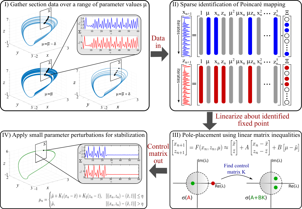
In Figure 1, we provide a visual illustration of the stabilization procedure, which is the focus of this article, applied to a fixed point of the Poincaré mapping. The method requires one to define a Poincaré section, $\Sigma$, that is transverse to the flow of a given nonlinear dynamical system and then obtain Poincaré section data, written compactly as the vector iterates ${{\bf x}}_{n}$, over a range of parameter values about a focal value, say $\bar{\mu}$. This gathered data represents the training data required to seed the SINDy method for the discovery of a parameter-dependent discrete dynamical system, ${\bf x}_{n+1}={\bf F}({\bf x}_{n},\mu)$, that maps iterates from one point in the Poincaré section to the next.

Supposing that we have identified a fixed point $\bar{\bf x}$ at $\mu=\bar{\mu}$, which corresponds to a UPO of the continuous-time dynamical system that we wish to stabilize¹¹ 1 The extension to stabilizing cyclic orbits of the Poincaré map is handled similarly later in the manuscript., we linearize the discovered mapping ${\bf F}$ about $({\bf x},\mu)=(\bar{\bf x},\bar{\mu})$, to obtain the Jacobian matrices evaluated at $(\bar{\bf x},\bar{\mu})$, ${\bf A}$ and ${\bf B}$, resulting from differentiation of ${\bf F}$ with respect to ${\bf x}$ and $\mu$, respectively. Since $\bar{\bf x}$ is taken to correspond to a UPO, it follows that at least one of the eigenvalues of ${\bf A}$ lies outside the unit circle in the complex plane, thus implying that the fixed point $\bar{\bf x}$ is linearly unstable. To stabilize this orbit, we apply the method of [36] by introducing small parameter manipulations at each intersection of the continuous-time trajectory with the Poincaré section. That is, we wish to obtain a control matrix ${\bf K}$ so that the eigenvalues of ${\bf A}+{\bf B}{\bf K}$ are entirely contained in the unit circle of the complex plane. Having found the matrix ${\bf K}$ we may then return to the original continuous-time dynamical system and apply the appropriate parameter manipulation each time the trajectory transversely intersects the Poincaré section. These parameter are described in detail in Section 3 as well as Figure 1.

From the above description of the stabilization algorithm, we see that obtaining an appropriate control matrix ${\bf K}$ to stabilize the trajectory is an important aspect of the procedure that must be informed by the linearization of the discovered mapping about the iterates of the UPO in the section. We note that there are a number of efficient methods which could be employed to finding the control matrix ${\bf K}$ [37, 38, 39, 40, 41, 42]. Here we opt to follow the methods of Parrilo [43] to see how the control matrix ${\bf K}$ can be obtained in a principled manner using linear matrix inequalities (LMIs). LMIs have long been applied to control systems [44] and have the advantage that they can be implemented numerically as semidefinite programs. This eases the analysis required by the user to stabilize UPOs since it does not require one to solve complicated nonlinear equations that may arise from attempting to find ${\bf K}$ by hand. Recent similar investigations have used Taylor expansions to obtain approximations of Poincaré mappings, while also employing LMIs to stabilize fixed points in the section [45, 46, 47, 48]. In this work we will extend the work of [43] to show that LMIs can be used to determine control matrices that stabilize cyclic orbits of the Poincaré mapping, going beyond just the original application to fixed points.

The rest of this paper is organized as follows. In Section 2 we present the SINDy method for discovering parameter-dependent Poincaré mappings. The presentation is supplemented with a brief historical overview of the method and a discussion of why the SINDy method is an appropriate model-discovery algorithm for the task at hand. Then in Section 3 we go over the LMI relaxation procedure of [43] for obtaining a control matrix ${\bf K}$. The original method for stabilizing fixed points of a mapping is presented in § 3.1, while our simple extension to cyclic orbits of a mapping is presented in § 3.2. Following these theoretical presentations of the two major components of the method, in Section 4 we present a number of applications. This includes demonstrating the utility of the LMI framework for stabilizing orbits of the chaotic Hénon map and then moving to the full algorithm which includes discovery of a Poincaré mapping. Our applications of the full method features a toy model which exhibits an isolated UPO and two chaotic systems, including the Rössler system. Section 5 briefly discusses how the method is adapted for parameter-independent models. The parameter-independent method is applied to a classical problem of having a satellite rest at an unstable Lagrange point of the Earth and its moon by applying discrete thrusts at regular temporal intervals. The paper concludes in Section 6 with a review of our findings and a discussion of some avenues for future work.

Given the flow ${\bf x}(t)$ of a continuous-time dynamical system, Poincaré proposed defining a lower-dimensional hyperplane $S$ that is transverse to this flow to simply track the intersection of the flow with $S$. The result of this process is a discrete sequence

$$\{{\bf x}_{n}={\bf x}(t_{n}):\ {\bf x}(t_{n})\in S,\ t_{n}>t_{n-1}\}$$

(2.1)

which comprise the successive iterates in the section. As discussed in the introduction, we are interested in parameter-dependent dynamics and therefore we will assume that such a sequence of iterates in a Poincaré section can be obtained over a range of parameter values, leading to the discrete sequences of data snapshots $\{{\bf x}_{1}^{(j)},\dots,{\bf x}_{N_{j}}^{(j)}\}\subset\mathbb{R}^{d}$ for the sampled parameter values $\mu_{j}\in\mathbb{R}^{p}$ with $j=1,\dots,M$. Our goal is to determine a parameter-dependent mapping so that when $\mu=\mu_{j}$ we map vectors ${\bf x}_{n}^{(j)}$ to ${\bf x}_{n+1}^{(j)}$. Such a mapping is referred to as a Poincaré mapping since it maps successive iterates of the Poincaré section into each other. As noted in the introduction, explicit representations of Poincaré mappings are rarely obtained for systems of interest. Therefore, we will leverage the model discovery algorithm SINDy [28, 29] to discover these parameter-dependent mappings.

We may begin by augmenting the data to incorporate the parameter as an extra $p$-variables in the training data. For each $j=1,\dots,M$ we consider the sequences $\{({\bf x}_{1}^{(j)},\mu_{j}),\dots,({\bf x}_{N_{j}}^{(j)},\mu_{j})\}\subset\mathbb{R}^{d}\times\mathbb{R}^{p}$ with the assumption that $({\bf x}_{n}^{(j)},\mu_{j})\mapsto({\bf x}_{n+1}^{(j)},\mu_{j})$, i.e. the parameter dynamics are trivial. We refer to this mapping as ${\bf F}:\mathbb{R}^{d}\times\mathbb{R}^{p}\to\mathbb{R}^{d}\times\mathbb{R}^{p}$ throughout this section. To discover ${\bf F}$ we apply SINDy, which frames model discovery as a sparse regression problem. We first stack the data into matrices

$${\bf X}_{1}:=\begin{bmatrix}{\bf x}_{1}^{(1)}&\mu_{1}\\ \vdots&\vdots\\ {\bf x}_{N_{1}-1}^{(1)}&\mu_{1}\\ {\bf x}_{1}^{(2)}&\mu_{2}\\ \vdots&\vdots\\ {\bf x}_{N_{2}-1}^{(2)}&\mu_{2}\\ \vdots&\vdots\\ {\bf x}_{1}^{(M)}&\mu_{M}\\ \vdots&\vdots\\ {\bf x}_{N_{M}-1}^{(M)}&\mu_{M}\end{bmatrix},\quad{\bf X}_{2}:=\begin{bmatrix}{\bf x}_{2}^{(1)}&\mu_{1}\\ \vdots&\vdots\\ {\bf x}_{N_{1}}^{(1)}&\mu_{1}\\ {\bf x}_{2}^{(2)}&\mu_{2}\\ \vdots&\vdots\\ {\bf x}_{N_{2}}^{(2)}&\mu_{2}\\ \vdots&\vdots\\ {\bf x}_{2}^{(M)}&\mu_{M}\\ \vdots&\vdots\\ {\bf x}_{N_{M}}^{(M)}&\mu_{M}\end{bmatrix}$$

(2.2)

belonging to $\mathbb{R}^{(N-M)\times(d+p)}$, where $N=\sum_{j=1}^{M}N_{j}$. From the assumptions on the data $({\bf x}_{n}^{(j)},\mu_{j})$, by construction ${\bf F}$ maps each row of ${\bf X}_{1}$ into the same row of ${\bf X}_{2}$. Although ${\bf F}$ is unknown, we may construct a library of $q\geq 1$ candidate functions for which ${\bf F}$ belongs to the linear span of these functions. Let us denote these candidate model functions ${\bf\theta}_{1},\dots,{\bf\theta}_{q}:\mathbb{R}^{d+p}\to\mathbb{R}^{d+p}$ so that the assumption ${\bf F}\in\mathrm{span}\{{\bf\theta}_{1},\dots,{\bf\theta}_{q}\}$ becomes

$${\bf F}({\bf x},\mu)={\bf\xi}_{1}{\bf\theta}_{1}({\bf x},\mu)+\dots+{\bf\xi}_{q}{\bf\theta}_{q}({\bf x},\mu)$$

(2.3)

where the ${\bf\xi}_{1},\dots,{\bf\xi}_{q}\in\mathbb{R}$ make up the coefficients in the linear span. For example, with $d=p=1$, one could consider polynomial basis functions up to quadratic order in a single variable $x$ and a single parameter $\mu$, thus giving a library of the form

$$\begin{bmatrix}1\\ 0\end{bmatrix},\begin{bmatrix}x\\ 0\end{bmatrix},\begin{bmatrix}\mu\\ 0\end{bmatrix},\begin{bmatrix}0\\ \mu\end{bmatrix},\begin{bmatrix}x^{2}\\ 0\end{bmatrix},\begin{bmatrix}\mu x\\ 0\end{bmatrix},\begin{bmatrix}\mu^{2}\\ 0\end{bmatrix},$$

(2.4)

where we remind the reader that the parameter dynamics, i.e. the second component, are assumed to be trivial. Due to these trivial parameter dynamics, we do not include them in our description of the discovered mappings in the applications that follow.

Now, we can couple the assumption (2.3) and the fact that rows of ${\bf X}_{1}$ are mapped by ${\bf F}$ into rows of ${\bf X}_{2}$. Take the first row as a specific example. Then, by assumption we have

$$\begin{bmatrix}{\bf x}_{2}\\ \mu_{1}\end{bmatrix}={\bf\xi}_{1}{\bf\theta}_{1}({\bf x}_{1},\mu_{1})+\dots+{\bf\xi}_{q}{\bf\theta}_{q}({\bf x}_{1},\mu_{1}),$$

(2.5)

giving a linear equation for the coefficients ${\bf\Xi}=[{\bf\xi}_{1}\ \dots\ {\bf\xi}_{q}]^{T}\in\mathbb{R}^{q}$. We can repeat this process for each row of ${\bf X}_{1}$ and ${\bf X}_{2}$, resulting in the linear system

$${\bf X}_{2}={\bf\Theta}({\bf X}_{1}){\bf\Xi}$$

(2.6)

where

$$\begin{split}&{\bf\Theta}({\bf X}_{1})\\ &=\begin{bmatrix}{\bf\theta}_{1}({\bf x}_{1}^{(1)},\mu_{1})&{\bf\theta}_{2}({\bf x}_{1}^{(1)},\mu_{1})&\cdots&{\bf\theta}_{q}({\bf x}_{1}^{(1)},\mu_{1})\\ \vdots&\vdots&\ddots&\vdots\\ {\bf\theta}_{1}({\bf x}_{N_{1}-1}^{(1)},\mu_{1})&{\bf\theta}_{2}({\bf x}_{N_{1}-1}^{(1)},\mu_{1})&\cdots&{\bf\theta}_{q}({\bf x}_{N_{1}-1}^{(1)},\mu_{1})\\ {\bf\theta}_{1}({\bf x}_{1}^{(2)},\mu_{2})&{\bf\theta}_{2}({\bf x}_{1}^{(2)},\mu_{2})&\cdots&{\bf\theta}_{q}({\bf x}_{1}^{(2)},\mu_{2})\\ \vdots&\vdots&\ddots&\vdots\\ {\bf\theta}_{1}({\bf x}_{N_{2}-1}^{(2)},\mu_{2})&{\bf\theta}_{2}({\bf x}_{N_{2}-1}^{(2)},\mu_{2})&\cdots&{\bf\theta}_{q}({\bf x}_{N_{2}-1}^{(2)},\mu_{2})\\ \vdots&\vdots&\ddots&\vdots\\ {\bf\theta}_{1}({\bf x}_{1}^{(M)},\mu_{M})&{\bf\theta}_{2}({\bf x}_{1}^{(M)},\mu_{M})&\cdots&{\bf\theta}_{q}({\bf x}_{1}^{(M)},\mu_{M})\\ \vdots&\vdots&\ddots&\vdots\\ {\bf\theta}_{1}({\bf x}_{N_{M}-1}^{(M)},\mu_{M})&{\bf\theta}_{2}({\bf x}_{N_{M}-1}^{(M)},\mu_{M})&\cdots&{\bf\theta}_{q}({\bf x}_{N_{M}-1}^{(M)},\mu_{M})\\ \end{bmatrix}\end{split}$$

(2.7)

is a matrix of the library functions evaluated at the entries of ${\bf X}_{1}$.

In practice we require a large number of measurements for each parameter value, thus giving that $N-M\gg 1$ and making (2.6) an overdetermined linear system. The early works of Small et al. [49] and Yao and Bollt [50] formulated model discovery in a similar manner resulting in models that potentially include all candidate functions after solving for ${\bf\Xi}$. The over-determined linear system (2.6) has a number of regularized solutions, but in practice our goal is to have the mapping ${\bf F}$ written as the linear span of as few candidate functions as possible, so a sparseness requirement can be imposed on the coefficients of ${\bf\Xi}$. In the present context, this sparsity requirement is motivated by the following three points: 1) many physical systems can be written in a sparse basis of candidate functions, 2) using fewer candidate functions to describe ${\bf F}$ will make the discovered mapping easier to analyze in what follows, and 3) promoting sparsity will help to eradicate small terms in the solution of (2.6) which could be attributed to numerical error in the training data.

There are many variants of sparse regression that could be employed to solve (2.6), all of which attempt to approximate the solution of an NP-hard $\ell_{0}$-optimization process [51]. In this manuscript we employ sequential threshold least squares [29] which is a proxy for $\ell_{0}$-optimization [52], has convergence guarantees [53], and out performs LASSO [54, 55] in most cases at significantly reduced computational expense. To apply this method we begin with the least-squares solution of (2.6), i.e. minimizing $\|{\bf X}_{2}-{\bf\Theta}({\bf X}_{1}){\bf\Xi}\|_{2}$ in ${\bf\Xi}=[{\bf\xi}_{1}\ \dots\ {\bf\xi}_{q}]\in\mathbb{R}^{q}$. We then introduce a sparsity threshold, $\lambda>0$ and define a new unknown matrix $\tilde{{\bf\Xi}}=[\tilde{\bf\xi}_{1}\ \dots\ \tilde{\bf\xi}_{q}]\in\mathbb{R}^{q}$ with $\tilde{{\bf\xi}}_{j}=0$ if the least-squares solution ${\bf\Xi}$ is such that $|{\bf\xi}_{j}|\leq\lambda$. This then moves one to another overdetermined linear system of equations

$${\bf X}_{2}={\bf\Theta}({\bf X}_{1})\tilde{\bf\Xi}$$

(2.8)

which potentially has fewer degrees of freedom due to fixing some coefficients of $\tilde{\bf\Xi}$ to zero. We then repeat the procedure by obtain the least-squares solution of (2.8) with the dimensionally-reduced vector $\tilde{{\bf\Xi}}$. This process is iterated with $\tilde{{\bf\Xi}}$ replacing ${\bf\Xi}$ until a sufficiently sparse model is obtained.

When implementing the above method there are two major components that must be chosen prior to implementing the method: the candidate functions which make up the library and the sparsity parameter. The choice of these two pieces of the method are intimately related. For example, one can image a scenario where the true mapping contains a trigonometric term, while the library consists solely of monomials. It is not unreasonable to suppose that the discovered mapping would attempt to build a series representation of the trigonometric term and the choice of the sparsity parameter effectively tells the discovery process where to truncate this series. Of course, taking $\lambda$ too large will provide too few terms in the series, while taking $\lambda$ too small has the potential to allow numerical error in cultivating the training data to manifest itself as small coefficients on library functions that should not be present in the discovered mapping. Conversely, including the appropriate trigonometric term in the library of functions could potentially provide greater forgiveness when choosing a value for $\lambda$. Such a phenomenon was exemplified in [30, Section IV C] where polynomial terms were used to approximate dynamics governed by a sine function. It can be a difficult task choosing the appropriate functions to include in the library of candidate functions and at the time of writing this manuscript there does not appear to be any prescriptions that are broadly applicable. Although this is a potential limitation of the method, we will see in Section 4 that for the examples considered herein, using a simple library of monomials can reliably capture the qualitative dynamics of a desired Poincaré mapping.

We conclude this section with the following remark. If there is a particular parameter value of interest, say $\bar{\mu}$, that one wishes to focus their analysis in a neighbourhood of, it may be advantageous to the discovery process to centre the parameter about this value. That is, one may introduce $\tilde{\mu}=\mu-\bar{\mu}$ and discover a mapping as a function of $\tilde{\mu}$ instead of $\mu$. The advantage this poses is that it can potentially maintain that the coefficients in the discovered mapping are kept relatively small and therefore the sparsity-promoting procedure can be more effective. To illustrate, consider the simple caricature

$$(\mu-10)^{3}=\mu^{3}+30\mu^{2}+300\mu+1000,$$

(2.9)

where we can see that centring the parameter about $\bar{\mu}=10$ results in a small single coefficient on $\tilde{\mu}^{3}=(\mu-10)^{3}$, whereas on the right the coefficients in powers of $\mu$ stretch across four orders of magnitude. Hence, not centring the parameter about $\bar{\mu}=10$ has the potential to lead to numerical error and ill-conditioning of the problem. In what follows we will apply this centring procedure whenever applicable.

In this section, we will actively adjust the parameter value $\mu$ to control the behavior of the system using full-state feedback control [37, 41, 42]. From the previous section, we may obtain a smooth, parsimonious, parameter-dependent mapping ${\bf F}:\mathbb{R}^{d}\times\mathbb{R}^{p}\to\mathbb{R}^{d}$ which faithful captures the iterates in a Poincaré section by

$${\bf x}_{n+1}={\bf F}({\bf x}_{n},\mu),$$

(3.1)

for all $n\geq 0$. Assuming that at some $\bar{\mu}\in\mathbb{R}^{p}$ the map (3.1) has a fixed point $\bar{{\bf x}}\in\mathbb{R}^{d}$, i.e. $\bar{{\bf x}}={\bf F}(\bar{{\bf x}},\bar{\mu})$, we may linearize the mapping about this fixed point to obtain

$${\bf x}_{n+1}-\bar{{\bf x}}\approx{\bf A}({\bf x}_{n}-\bar{{\bf x}})+{\bf B}(\mu_{n}-\bar{\mu})$$

(3.2)

where

$${\bf A}:={\bf F}_{x}(\bar{{\bf x}},\bar{\mu})\in\mathbb{R}^{d\times d},\quad{\bf B}:={\bf F}_{\mu}(\bar{{\bf x}},\bar{\mu})\in\mathbb{R}^{d\times p}.$$

(3.3)

are the Jacobian matrices of (3.1) resulting from differentiation with respect to ${\bf x}$ and $\mu$, respectively. When ${\bf x}_{n}$ is in a neighbourhood of $\bar{{\bf x}}$, we will use the parameter fluctuations $\mu_{n}$ to control the system by making them linear functions of the state variable ${\bf x}$, whereas when ${\bf x}$ is far from $\bar{{\bf x}}$ we will simply take $\mu_{n}=\bar{\mu}$. That is,

$$\mu_{n}=\begin{cases}\bar{\mu}+{\bf K}({\bf x}_{n}-\bar{{\bf x}})&|{\bf x}_{n}-\bar{{\bf x}}|\leq\eta\\ \bar{\mu}&|{\bf x}_{n}-\bar{{\bf x}}|>\eta\end{cases}$$

(3.4)

for a yet-to-be specified control matrix ${\bf K}\in\mathbb{R}^{p\times d}$ and some $\eta>0$ which we refer to as the threshold parameter. Notice that for ${\bf x}_{n}$ in a neighbourhood of $\bar{{\bf x}}$ with the parameter choices in (3.4) the linearization (3.2) becomes

$${\bf x}_{n+1}-\bar{{\bf x}}\approx({\bf A}+{\bf B}{\bf K})({\bf x}_{n}-\bar{{\bf x}}),$$

(3.5)

and so our goal now becomes choosing the matrix ${\bf K}$ in such a way that every iterate of the linearized mapping (3.5) converges to $\bar{{\bf x}}$ as $n\to\infty$. This approach is known as full state feedback control in the field of control theory, and there are well known solutions [37, 41, 42, 40].

We will refer to a matrix ${\bf M}\in\mathbb{R}^{d\times d}$ as stable if all eigenvalues $\lambda\in\mathbb{C}$ are such that $|\lambda|<1$ and note that this implies that every solution of the linear mapping ${\bf x}_{n+1}={\bf M}{\bf x}_{n}$ converges to zero as $n\to\infty$, regardless of initial condition. We make use of the following Lyapunov characterization which gives an equivalent condition for the stability of a matrix:

$${\bf M}\mathrm{\ is\ stable}\iff\exists{\bf P}\succ 0\ \mathrm{s.t.}\ {\bf P}-{\bf M}^{T}{\bf P}{\bf M}\succ 0.$$

(3.6)

Here the subscript $T$ denotes the matrix transpose and ${\bf P}\succ 0$ denotes that ${\bf P}$ is positive definite. Returning to (3.5), a matrix ${\bf K}$ making $({\bf A}+{\bf B}{\bf K})$ stable is then equivalent to saying that there exists a ${\bf P}\succ 0$ such that

$${\bf P}-({\bf A}+{\bf B}{\bf K})^{T}{\bf P}({\bf A}+{\bf B}{\bf K})\succ 0.$$

(3.7)

Notice that to solve (3.7) we are required to obtain both ${\bf K}$ and ${\bf P}$, thus making the left-hand-side nonlinear in the unknowns. In § 3.1 we present Parrilo’s method for obtaining a matrix ${\bf K}$ that makes ${\bf A}+{\bf B}{\bf K}$ stable by converting (3.7) to an equivalent LMI [43]. Such an LMI can be evaluated numerically as a semidefinite program. In § 3.2 we provide a simple extension of these methods to cyclic orbits.

Prior to presenting the equivalent LMI formulation for solving (3.7), we note that the process of obtaining a matrix ${\bf K}$ is referred to as the pole-placement method. Pole-placement is a standard approach in feedback control [37, 38, 39] to design a control matrix ${\bf K}$ to obtain arbitrary placement of the eigenvalues of the closed-loop system ${\bf A}+{\bf B}{\bf K}$. Pole placement has already been proposed by Romeiras et al. [36] for the control of chaos. The arbitrary placement of the closed-loop eigenvalues is possible if and only if the system is controllable [37, 40], meaning that the Krylov subspace spanned by ${\bf A}$ and ${\bf B}$ has full row rank. One common pole placement is obtained via a linear quadratic regulator (LQR) that minimizes an infinite-time horizon cost function

$$J=\sum_{n=0}^{\infty}({\bf x}_{n}-\bar{\bf x})^{T}{\bf J}_{1}({\bf x}_{n}-\bar{\bf x})+(\mu_{n}-\bar{\mu})^{T}{\bf J}_{2}(\mu_{n}-\bar{\mu}),\quad{\bf J}_{1}\succeq 0,{\bf J}_{2}\succ 0.$$

(3.8)

In this case, the unique matrix ${\bf K}$ balances the aggressiveness of stabilization with control expenditure, and is obtained by solving a Riccati equation [40]. Notice that the value of $\eta$ can be used to control the value of any cost function in the form (3.8) since the control of the nonlinear mapping (3.1) is only turned on in a small neighbourhood of $\bar{\bf x}$. Hence, we will not assume that a cost function is given since we may simply decrease the value of $\eta$ to decrease the strength of the control applied to the system. On the other end, the maximal allowable value of $\eta>0$ is intimately related to the choice of ${\bf K}$ since it must be chosen to lie in the basin of attraction of $\bar{{\bf x}}$ to the nonlinear mapping (3.1) after implementing the parameter control (3.4). We therefore require that $|{\bf K}({\bf x}_{n}-\bar{{\bf x}})|$ is sufficiently small to guarantee that $\mu_{n}$ remains in a neighbourhood of $\bar{\mu}$. We refer the reader to [26, 36] for a more complete discussion of the choice of the threshold parameter as it relates to the control matrix ${\bf K}$.

In this section we will provide illustrative examples of utility of our methods. All numerical procedures are implemented in MATLAB R2019a, while a robust python-based SINDy package (PySindy) [56] is publicly available at GitHub/dynamicslab/pysindy. Throughout this section our library of candidate functions will consist of all monomials up to degree 5 in the Poincaré section variables. We use the MATLAB software YALMIP (version R20190425) [57] to solve the LMIs that determine the control matrices using the numerical implementation (3.12). All code for this section is available at GitHub/jbramburger/Stabilizing_UPOs. Finally, throughout this section we refer to period $m\geq 1$ orbits for continuous dynamical systems as periodic solutions which intersect the Poincaré section at $m$ distinct points, i.e. $m$-cycles. This is in contrast to the definition that the temporal period of the orbits is the integer $m$ which may be a source of confusion for the reader.

References

- [1] L. Devaney and R. Devaney. An Introduction To Chaotic Dynamical Systems, Second Edition. Addison-Wesley advanced book program. Avalon Publishing, 1989.
- [2] Edward Ott. Chaos in Dynamical Systems. Cambridge University Press, 2 edition, 2002.
- [3] R Artuso, E Aurell, and P Cvitanovic. Recycling of strange sets: I. cycle expansions. Nonlinearity, 3(2):325–359, may 1990.
- [4] Ditza Auerbach, Predrag Cvitanović, Jean-Pierre Eckmann, Gemunu Gunaratne, and Itamar Procaccia. Exploring chaotic motion through periodic orbits. Phys. Rev. Lett., 58:2387–2389, Jun 1987.
- [5] Predrag Cvitanović. Invariant measurement of strange sets in terms of cycles. Phys. Rev. Lett., 61:2729–2732, Dec 1988.
- [6] N. B. Budanur, K. Y. Short, M. Farazmand, A. P. Willis, and P. Cvitanović. Relative periodic orbits form the backbone of turbulent pipe flow. Journal of Fluid Mechanics, 833:274–301, 2017.
- [7] P Cvitanović and J F Gibson. Geometry of the turbulence in wall-bounded shear flows: periodic orbits. Physica Scripta, T142:014007, dec 2010.
- [8] L. Fazendeiro, B.M. Boghosian, P.V. Coveney, and J. Lätt. Unstable periodic orbits in weak turbulence. Journal of Computational Science, 1(1):13 – 23, 2010.
- [9] Valter Franceschini and Claudio Tebaldi. Sequences of infinite bifurcations and turbulence in a five-mode truncation of the navier-stokes equations. Journal of Statistical Physics, 21(6):707–726, 1979.
- [10] Dan Lucas and C. P. Caulfield. Irreversible mixing by unstable periodic orbits in buoyancy dominated stratified turbulence. Journal of Fluid Mechanics, 832:R1, 2017.
- [11] Valery Petrov, Michael F Schatz, Kurt A Muehlner, Stephen J VanHook, WD McCormick, JB Swift, and Harry L Swinney. Nonlinear control of remote unstable states in a liquid bridge convection experiment. Physical review letters, 77(18):3779, 1996.
- [12] Bruno Eckhardt, Tobias M Schneider, Bjorn Hof, and Jerry Westerweel. Turbulence transition in pipe flow. Annu. Rev. Fluid Mech., 39:447–468, 2007.
- [13] Gökhan Yalniz, Björn Hof, and Nazmi Burak Budanur. Coarse graining the state space of a turbulent flow using periodic orbits, 2020.
- [14] Balachandra Suri, Logan Kageorge, Roman O Grigoriev, and Michael F Schatz. Capturing turbulent dynamics and statistics in experiments with unstable periodic orbits. Physical Review Letters, 125(6):064501, 2020.
- [15] Michael D Graham and Daniel Floryan. Exact coherent states and the nonlinear dynamics of wall-bounded turbulent flows. Annual Review of Fluid Mechanics, 53, 2020.
- [16] Wang Sang Koon, Martin W Lo, Jerrold E Marsden, and Shane D Ross. Heteroclinic connections between periodic orbits and resonance transitions in celestial mechanics. Chaos: An Interdisciplinary Journal of Nonlinear Science, 10(2):427–469, 2000.
- [17] Gerard Gómez, Wang S Koon, MW Lo, Jerrold E Marsden, Josep Masdemont, and Shane D Ross. Connecting orbits and invariant manifolds in the spatial restricted three-body problem. Nonlinearity, 17(5):1571, 2004.
- [18] M. Dellnitz, O. Junge, W. S. Koon, F. Lekien, M. W. Lo, J. E. Marsden, K. Padberg, R. Preis, S. D. Ross, and B. Thiere. Transport in dynamical astronomy and multibody problems. International Journal of Bifurcation and Chaos, 15:699–727, 2005.
- [19] Edward Ott, Celso Grebogi, and James A. Yorke. Controlling chaos. Phys. Rev. Lett., 64:1196–1199, Mar 1990.
- [20] J N Weiss, A Garfinkel, M L Spano, and W L Ditto. Chaos and chaos control in biology. The Journal of Clinical Investigation, 93(4):1355–1360, 4 1994.
- [21] Alexander Fradkov and Boris Andrievsky. Methods and examples of controlling chaos in mechanical systems. In G. Rega and F. Vestroni, editors, IUTAM Symposium on Chaotic Dynamics and Control of Systems and Processes in Mechanics, pages 481–491, Dordrecht, 2005. Springer Netherlands.
- [22] Xiaoxin Liao and Pei Yu. Application to Chaos Control and Chaos Synchronization, pages 337–369. Springer Netherlands, Dordrecht, 2008.
- [23] Yousef Farid and Tahmine Vedadi Moghaddam. Generalized projective synchronization of chaotic satellites problem using linear matrix inequality. International Journal of Dynamics and Control, 2(4):577–586, 2014.
- [24] B. R. Andrievskii and A. L. Fradkov. Control of chaos: Methods and applications. i. methods. Automation and Remote Control, 64(5):673–713, 2003.
- [25] B. R. Andrievskii and A. L. Fradkov. Control of chaos: Methods and applications. ii. applications. Automation and Remote Control, 65(4):505–533, 2004.
- [26] S. Boccaletti, C. Grebogi, Y.-C. Lai, H. Mancini, and D. Maza. The control of chaos: theory and applications. Physics Reports, 329(3):103 – 197, 2000.
- [27] Alexander L. Fradkov and Robin J. Evans. Control of chaos: Methods and applications in engineering. Annual Reviews in Control, 29(1):33 – 56, 2005.
- [28] Jason J. Bramburger and J. Nathan Kutz. Poincaré maps for multiscale physics discovery and nonlinear floquet theory. Physica D: Nonlinear Phenomena, 408:132479, 2020.
- [29] Steven L. Brunton, Joshua L. Proctor, and J. Nathan Kutz. Discovering governing equations from data by sparse identification of nonlinear dynamical systems. Proceedings of the National Academy of Sciences, 113(15):3932–3937, 2016.
- [30] Jason J. Bramburger, Daniel Dylewsky, and J. Nathan Kutz. Sparse identification of slow timescale dynamics. Phys. Rev. E, 102:022204, Aug 2020.
- [31] Kathleen P. Champion, Steven L. Brunton, and J. Nathan Kutz. Discovery of nonlinear multiscale systems: Sampling strategies and embeddings. SIAM Journal on Applied Dynamical Systems, 18(1):312–333, 2019.
- [32] Samuel H. Rudy, Steven L. Brunton, Joshua L. Proctor, and J. Nathan Kutz. Data-driven discovery of partial differential equations. Science Advances, 3(4), 2017.
- [33] Daniel E. Shea, Steven L. Brunton, and J. Nathan Kutz. Sindy-bvp: Sparse identification of nonlinear dynamics for boundary value problems, 2020.
- [34] Kadierdan Kaheman, J. Nathan Kutz, and Steven L. Brunton. Sindy-pi: A robust algorithm for parallel implicit sparse identification of nonlinear dynamics. CoRR, abs/2004.02322, 2020.
- [35] Eurika Kaiser, J. Nathan Kutz, and Steven L. Brunton. Discovering conservation laws from data for control. In 57th IEEE Conference on Decision and Control, CDC 2018, Miami, FL, USA, December 17-19, 2018, pages 6415–6421. IEEE, 2018.
- [36] Filipe J. Romeiras, Celso Grebogi, Edward Ott, and W.P. Dayawansa. Controlling chaotic dynamical systems. Physica D: Nonlinear Phenomena, 58(1):165 – 192, 1992.
- [37] G. Dullerud and Fernando Paganini. A course in robust control theory: A convex approach. 2005.
- [38] K. Ogata. Modern Control Engineering. Instrumentation and controls series. Prentice Hall, 2010.
- [39] E.D. Sontag. Mathematical Control Theory: Deterministic Finite Dimensional Systems. Texts in Applied Mathematics. Springer New York, 2013.
- [40] Steven L. Brunton and J. Nathan Kutz. Data-Driven Science and Engineering: Machine Learning, Dynamical Systems, and Control. Cambridge University Press, 2019.
- [41] S. Skogestad and I. Postlethwaite. Multivariable feedback control: analysis and design. John Wiley & Sons, Inc., Hoboken, New Jersey, 2 edition, 2005.
- [42] Karl Johan Aström and Richard M Murray. Feedback systems: an introduction for scientists and engineers. Princeton university press, 2010.
- [43] Pablo A. Parrilo. Chapter 2: Semidefinite Optimization, pages 3–46.
- [44] Stephen Boyd, Laurent El Ghaoui, Eric Feron, and Venkataramanan Balakrishnan. Linear Matrix Inequalities in System and Control Theory. Society for Industrial and Applied Mathematics, 1994.
- [45] Wafa Znegui, Hassène Gritli, and Safya Belghith. Design of an explicit expression of the poincaré map for the passive dynamic walking of the compass-gait biped model. Chaos, Solitons & Fractals, 130:109436, 2020.
- [46] Wafa Znegui, Hassène Gritli, and Safya Belghith. Stabilization of the passive walking dynamics of the compass-gait biped robot by developing the analytical expression of the controlled poincarémap. Nonlinear Dynamics, 101(2):1061–1091, 2020.
- [47] Wafa Znegui, Hassène Gritli, and Safya Belghith. A new poincaré map for investigating the complex walking behavior of the compass-gait biped robot. Applied Mathematical Modelling, 94:534–557, 2021.
- [48] Hassène Gritli. Poincaré maps design for the stabilization of limit cycles in non-autonomous nonlinear systems via time-piecewise-constant feedback controllers with application to the chaotic duffing oscillator. Chaos, Solitons & Fractals, 127:127–145, 2019.
- [49] Michael Small, Kevin Judd, and Alistair Mees. Modeling continuous processes from data. Phys. Rev. E, 65:046704, Apr 2002.
- [50] Chen Yao and Erik M. Bollt. Modeling and nonlinear parameter estimation with kronecker product representation for coupled oscillators and spatiotemporal systems. Physica D: Nonlinear Phenomena, 227(1):78 – 99, 2007.
- [51] B. K. Natarajan. Sparse approximate solutions to linear systems. SIAM Journal on Computing, 24(2):227–234, 1995.
- [52] P. Zheng, T. Askham, S. L. Brunton, J. N. Kutz, and A. Y. Aravkin. A unified framework for sparse relaxed regularized regression: Sr3. IEEE Access, 7:1404–1423, 2019.
- [53] Linan Zhang and Hayden Schaeffer. On the convergence of the sindy algorithm. Multiscale Modeling & Simulation, 17(3):948–972, 2019.
- [54] Weijie Su, Magorzata Bogdan, and Emmanuel Candès. False discoveries occur early on the lasso path. Ann. Statist., 45(5):2133–2150, 10 2017.
- [55] Robert Tibshirani. Regression shrinkage and selection via the lasso. Journal of the Royal Statistical Society. Series B (Methodological), 58(1):267–288, 1996.
- [56] Brian M. de Silva, Kathleen Champion, Markus Quade, Jean-Christophe Loiseau, J. Nathan Kutz, and Steven L. Brunton. Pysindy: A python package for the sparse identification of nonlinear dynamical systems from data. Journal of Open Source Software, 5(49):2104, 2020.
- [57] J. Löfberg. Yalmip : a toolbox for modeling and optimization in matlab. In 2004 IEEE International Conference on Robotics and Automation (IEEE Cat. No.04CH37508), pages 284–289, 2004.
- [58] M. Hénon. A two-dimensional mapping with a strange attractor. Comm. Math. Phys., 50(1):69–77, 1976.
- [59] Predrag Cvitanović, Gemunu H. Gunaratne, and Itamar Procaccia. Topological and metric properties of hénon-type strange attractors. Phys. Rev. A, 38:1503–1520, Aug 1988.
- [60] Tianshu Wang, Xingyuan Wang, and Mingjun Wang. Chaotic control of hénon map with feedback and nonfeedback methods. Communications in Nonlinear Science and Numerical Simulation, 16(8):3367 – 3374, 2011.
- [61] O.E. Rössler. An equation for continuous chaos. Physics Letters A, 57(5):397 – 398, 1976.
- [62] Roberto Barrio, Fernando Blesa, Angeles Dena, and Sergio Serrano. Qualitative and numerical analysis of the rössler model: Bifurcations of equilibria. Comput. Math. Appl., 62:4140–4150, 2011.
- [63] H.O. Peitgen, H. Jürgens, and D. Saupe. Chaos and Fractals: New Frontiers of Science. Springer New York, 2004.
- [64] J.C. Sprott. Simplest dissipative chaotic flow. Physics Letters A, 228(4):271 – 274, 1997.
- [65] Eurika Kaiser, J. Kutz, and Steven Brunton. Sparse identification of nonlinear dynamics for model predictive control in the low-data limit. Proceedings of the Royal Society A: Mathematical, Physical and Engineering Science, 474:20180335, 11 2018.
- [66] Paul So, Edward Ott, Tim Sauer, Bruce J. Gluckman, Celso Grebogi, and Steven J. Schiff. Extracting unstable periodic orbits from chaotic time series data. Phys. Rev. E, 55:5398–5417, May 1997.
- [67] Jacob Page and Rich R. Kerswell. Searching turbulence for periodic orbits with dynamic mode decomposition. Journal of Fluid Mechanics, 886:A28, 2020.
- [68] Mayur V. Lakshmi, Giovanni Fantuzzi, Jesús D. Fernández-Caballero, Yongyun Hwang, and Sergei I. Chernyshenko. Finding extremal periodic orbits with polynomial optimization, with application to a nine-mode model of shear flow. SIAM Journal on Applied Dynamical Systems, 19(2):763–787, 2020.
- [69] Eric Sidorov and Miriam Zacksenhouse. Lyapunov based estimation of the basin of attraction of poincare maps with applications to limit cycle walking. Nonlinear Analysis: Hybrid Systems, 33:179 – 194, 2019.
- [70] Edward N. Lorenz. Deterministic Nonperiodic Flow. Journal of the Atmospheric Sciences, 20(2):130–141, 03 1963.
- [71] B. R. Noack, K. Afanasiev, M. Morzynski, G. Tadmor, and F. Thiele. A hierarchy of low-dimensional models for the transient and post-transient cylinder wake. Journal of Fluid Mechanics, 497:335–363, 2003.
- [72] J.-C. Loiseau and S. L. Brunton. Constrained sparse Galerkin regression. Journal of Fluid Mechanics, 838:42–67, 2018.
- [73] J.-C. Loiseau, B. R. Noack, and S. L. Brunton. Sparse reduced-order modeling: sensor-based dynamics to full-state estimation. Journal of Fluid Mechanics, 844:459–490, 2018.
- [74] Jean-Christophe Loiseau. Data-driven modeling of the chaotic thermal convection in an annular thermosyphon. Theoretical and Computational Fluid Dynamics, 34(4):339–365, 2020.