Marina Meilă and Michael I. Jordan
Bayesian Importance of Features (BIF)
Abstract
We introduce a simple and intuitive framework that provides quantitative explanations of statistical models through the probabilistic assessment of input feature importance. The core idea comes from utilizing the Dirichlet distribution to define the importance of input features and learning it via approximate Bayesian inference. The learned importance has probabilistic interpretation and provides the relative significance of each input feature to a model’s output, additionally assessing confidence about its importance quantification. As a consequence of using the Dirichlet distribution over the explanations, we can define a closed-form divergence to gauge the similarity between learned importance under different models. We use this divergence to study the feature importance explainability tradeoffs with essential notions in modern machine learning, such as privacy and fairness. Furthermore, BIF can work on two levels: global explanation (feature importance across all data instances) and local explanation (individual feature importance for each data instance). We show the effectiveness of our method on a variety of synthetic and real datasets, taking into account both tabular and image datasets. The code is available at https://github.com/kamadforge/featimp_dp
keywords
Explainable AI, Interpretability, Feature Selection, Bayesian Inference, Privacy1 Introduction
The increasing spread of machine learning algorithms in a wide range of human domains prompt the public and regulatory bodies to increase scrutiny on the requirements on algorithmic design (Voigt and Bussche 2017). Among them, explainability aims to provide a human interpretable reasoning for algorithmic decisions (Goodman and Flaxman 2016). With the goal of gaining such explainability, there has been a large number of methods developed for explaining why machine learning models produce particular outputs (Ribeiro et al. 2016a; Lundberg and Lee 2017b). In this paper, we tackle the problem of accurately assessing how relevant each of the data input feature is to a machine learning model.
Broadly speaking, there are two levels at which one could gain such input feature explainability. The first level is global, where the goal is to identify the most relevant features for a given task globally across all the data instances. However, when the data exhibit a large variability, using global explanation methods is not suitable, as the learned feature importance at the global level is same for all data samples. To overcome this limitation, the second level is local, where the goal is to identify the most relevant features for each data instance separately (Shrikumar et al. 2017). The current literature proposes separate mechanisms for each of the approaches to feature explanations. The traditional feature selection literature offers a large number of methods for global explanations (Hall 1999; Hanchuan Peng et al. 2005; Candes et al. 2016; Guyon and Elisseeff 2003; Kira and Rendell 1992) while newer methods concentrate on instance-wise approaches (Chen et al. 2018; Yoon et al. 2018). On the other hand, BIF is a common framework which allows both for global and local explanation.
Providing local explanations is challenging and requires backing by an external model. The current approaches provide two ways for local explanations. The first group provides model-agnostic methods which rely on the outputs of common machine learning models (e.g. Random Forest or XGBoost). The second group concentrates on leveraging neural networks to build their own models which provide feature explanations. BIF is a novel method that bridges both approaches, additionally providing a Bayesian perspective for feature importance.
Thus, we introduce a framework called Bayesian importance of features (BIF) for gaining the explainability of complex machine learning models both globally and locally with the following benefits:
- •
It models feature importance via Dirichlet distribution thus providing probabilistic interpretation and relative weighing of the features.
- •
By means of Bayesian formulation, it provides the uncertainty measure of the assessed importance values.
- •
The algorithm produces the distribution over the feature importance, which we exploit to quantify the trade-offs between a model’s explainability in terms of the feature importance and other notions such as privacy and fairness.
- •
As a unified framework, it can learn a global probability over features via a simple model linear in the number of parameters, or apply neural networks to produce an instance-wise explanation.
- •
The proposed method is a flexible meta-algorithm which can work with any model through which we can backpropagate.
2 Related Work
Feature selection, overall, is intended to reduce the number of data input variables to those that are the most useful to a model in order to predict the target variable. The feature selection methods can be subdivided in various ways, supervised and unsupervised methods, or wrapper (which evaluate subsets of variables to maximize performance), filter (which evaluate the relationships between each input feature and the target) and embedded (such as penalized regression or random forest) methods (Kuhn et al. 2013). Feature importance, the issue which we tackle in this work, belongs to the filter-type methods. Alternatively, we may also distinguish two broad categories, feature-additive and feature-selection methods (Linardatos et al. 2021). Subsequently, methods can be divided into global explanations which assess the features for all the data, and local (or instance-wise) which provide the explanation for feature in each data instance.
Feature-additive methods provide importance of features per dimension, such that their sum matches a quantity of interest, typically the model’s output. Two popular such methods are LIME (Ribeiro et al. 2016b) and SHAP (Lundberg and Lee 2017a). LIME assumes that any complex model is linear locally. It fits a simple model around a single observation using new samples with permuted features, weighted according to their proximity to the original. SHAP is based on the game-theoretical concept of the Shapley value which assesses average marginal contribution of an input. SHAP, however, utilizes the reinterpretation from (Charnes et al. 1988) where the score is a weighted linear combination of features. This approach provides a local explanation by the level of deviation a given data sample gets from the global feature average. Both LIME and SHAP, similarily to BIF, provide a feature importance weight. Other notable feature additive approaches include attribution-based methods (Ancona et al. 2017) such as Integrated Gradient (Sundararajan et al. 2017), Smoothgrad (Smilkov et al. 2017).
On the other hand, feature-selection narrows down the set of features and finds a subset of input features which produce a similar result to the case when the full set of input features is used. Two recent such models are L2X (Chen et al. 2018) and INVASE (Yoon et al. 2018). One notable difference from the classical feature selection methods such as LASSO (Tibshirani 1996) is that these methods target instance-wise feature selection and build their own neural network-based pipeline. L2X maximizes the mutual information between subsets of features and the response variable , and approximates this quantity with a network which produces binary feature samples learnt via continuous relaxation with the Gumbel-softmax trick. INVASE (Yoon et al. 2018) consists of three networks. The first network is a selector network which provides selection probabilities given each input feature. However, unlike in our model, the outputs of the selector network are treated as separate Bernoulli variables and are not directly trained with the model’s output. The output of the selector network is fed into two separate networks which form an actor-critic pair for feature selection. Both of these methods produce binary output of important features: L2X outputs a predetermined set of important features while INVASE determines the based on a threshold.
3 Problem formulation
Generally, feature importance assigns a score to each input feature in the input data , where denotes the number of features and the number of data examples. For a given feature, the score can be the same or differ for each data sample , which is described by the two following concepts:
Global explanation: We assign a universal, -dimensional vector of values f to the set of input features in the dataset . The value quantifies the relevance or importance of the feature for the entire dataset. In particular, the vector assigns a single, scalar-valued global score to each feature .
Local explanation: Every instance of data is assigned a separate, -dimensional feature importance vector , and the importance vectors and for two different data instances and need not be the same.
Moreover, feature importance is computed in relation to a model . In other words, a feature is important for a task indicated by a model in question, denoted by , and thus we require a data-model tuple (). What comes next describes our method that provides probabilistic interpretation of both global and local explanations.
4 Methods: Bayesian importance of features (BIF)
Consider a data-model tuple () such that and is any differentiable model. That is, a model is trained with an -element dataset , where is an input datum, its label (either discrete or continuous) and is the input dimension. The proposed method assesses the importance of the set of input features given the model . Moreover, we aim to idenfity how each feature of the dataset affects the output of on two different levels.
4.1 Global explanation
In the global feature explanations, we assign the importance for a feature across the entire dataset. Usually, this value is unbounded (Lundberg and Lee 2017a) or binary. In our view, it is intuitive to describe the feature importance through a probability vector which describes the relative weight of a feature. Moreover, as we consider the data-model tuple (), the importance can be viewed as a contribution of a feature to the maximization of the objective function given by the model . In our method, we name the importance vector. This vector is used to perform the scalar product which becomes the new weighted input to the model . The mechanism is illustrated in Fig. 1.
Loss function for global explanation : Let denote the loss for obtaining the global feature importance and the probability of the data under a model . In our method, we assume a parametrized model of joint distribution between the data 11 1 We preserve the notation which is common in the literature, however one should note that in the derivations is an equivalent notation for a sample . For the global case, we omit the index for clarity. and the importance feature vector . In principle, we want to maximize the log-likelihood of the data which is obtained by integrating out the feature importance vector, Under a neural network model, directly integrating out is intractable. We instead use an approximate distribution , which approximates . Minimizing the KL-divergence between the two distributions is equivalent to maximizing the lower bound to the data log-likelihood:
| (1) |
Parameterization. The terms in are defined as follows:
| (2) | ||||
| (3) |
Both and are parameter vectors of the Dirichlet distribution. We set the parameters to some constant value and only optimize for . Assuming the Dirichlet distribution both for the posterior and the prior allows us to obtain a closed-form KL-divergence in Eq. 1. Thus, the objective function in Eq. 1 depends on the Dirichlet parameters :
| (4) |
The crucial characteristic of the global explanation when computing the loss is that for two samples, and , the importance vectors and are sampled from the same parameters Dir() across the entire dataset. In the above loss we use the likelihood of the model (that is which is computed with the output of the model ), but we do not alter the parameters of the model (which we assume to be pre-trained with ). We freeze its parameters, and only train the parameters of the feature importance vector . The algorithm for obtaining the global feature importance is summarized in Algorithm 122 2 Our algorithm is general for any classification (both binary and multi-class) and regression tasks. However, in our experiments we focus on the classification tasks..
Why Dirichlet? Dirichlet distribution describes a family of categorical distributions defined over a simplex, and a sample of the Dirichlet distribution is a probability vector, where all elements of are non-negative and This property makes it natural to model a relative level of importance across different input features. Moreover, the choice of Dirichlet distribution allows for the closed-form expression of KL-divergence.
4.2 Local or instance-wise explanation via Importance Network (IN)
Local explanations differ from the global ones in that feature importance is evaluated for each data instance. In global explanation, we only produce a single vector . Conversely, in the local setting, we produce an importance matrix. To be precise, each data point is assigned a vector indicating the feature importance for that particular data point. Thus, while , an importance matrix of size is generated.
Parameterization. In the case of local explanations, each of the importance vectors, is also modelled by the Dirichlet distribution with individual parameters ,
| (5) | ||||
| (6) |
where we set the parameters the same for all , as we do not have any prior knowledge on any particular data instances.
Importance network. The global importance vector tells us the average feature importance across all the data instances in the entire dataset. However, in the local case, we assign an importance vector for each data instance . To learn the mapping between the two, we resort to an additional model, an importance network (IN)33 3 In our experiments, we use a multi-layer feed-forward network. Note that other types of networks are also possible, e.g. convolutional neural networks can be more appropriate for image data. parameterized by . The importance network maps a data instance to a corresponding Dirichlet parameter vector , i.e., . And following Eq. 6, we draw a corresponding feature importance from the Dirichlet distribution with the parameter . Hence, the IN model can produce an individual feature importance for each data instance (via Dirichlet parameters).
Similarly to the global case, we again use the variational lower bound. However, in the local case, our new objective function over for all become dependent on the parameters of the importance network:
| (7) | ||||
During training, we set to a fixed value and optimize for . Given a sample , we apply an element-wise multiplication, , which is fed to the model in question . The model then produces the conditional distribution . During learning as in the global case, we do not update the parameters of , but only update the parameters of the IN model. We summarize our algorithm in Algorithm 2 and provide the graphical depiction of this process in Fig. 1 (black box).
4.3 Sampling vs. a point estimate
Sampling.
In both objective functions, Eq. 1 and Eq. 7, in the left-hand side term (so called, cross-entropy term) we need to evaluate an integral over (or ). We do so by the Monte Carlo integration using Eq. 3 for the global setting and Eq. 6 for the local setting. The integral is evaluated for each data input (we use here the data index to describe both the global and the local case):
| (8) |
where the subscript denotes the th Monte Carlo sample from the Dirichlet distribution . Following (Knowles 2015), we compute the gradients of the integral implicitly using the inverse CDF of the Gamma distribution.
A point estimate.
A computationally cheap approximation to the integral is using the analytic mean expression of the Dirichlet random variables,
| (9) |
where Computing the point estimate does not require sampling and propagating gradients through the samples, which significantly reduces the run time. In our experiments, we use both approximations where the specifics on each approximation are included in the Supplementary material.
4.4 Divergence for measuring similarity under BIF
The BIF’s output, the Dirichlet distribution is an exponential family distribution, which we can write in terms of an inner product between the sufficient statistic and the natural parameter :
| (10) |
where is the log-partition function, and is the base measure. In case of the Dirichlet distribution, the natural parameter equals the parameter , yielding a canonical form.
We are interested in measuring how similar feature importance is under two different models. We denote the two Dirichlet distributions for feature importance obtained under the two models by and , respectively, where ’s parameters are and ’s are . Luckily under the exponential family distribution, popular divergence definitions such as the KL divergence and the Bregman divergence can be expressed in terms of the log-partition function, its parameter, and the expected sufficient statistic:
| (11) |
where is the expected sufficient statistic under the distribution . Under the Dirichlet distribution, all of the three terms are in closed-form, where the log-partition function is defined by , where denotes Gamma distribution, and each coordinate of the expected sufficient statistic is defined by , where is the digamma function. This allows us to evaluate the KL divergence conveniently. We demonstrate how we take advantage of having this easy-to-evaluate divergence in practice and examine the results under BIF in Sec. 5.
5 Experiments
| Syn 1 | Syn 2 | Syn 3 | Syn 4 | Syn 5 | Syn 6 | |
|---|---|---|---|---|---|---|
| BIF (global) | 85.0 | - | - | - | ||
| BIF (inst, samp) | 93.6 | 81.9 | 85.2 | |||
| BIF (inst, pe) | 82.9 | 79.0 | ||||
| L2X | 66.0 | 64.5 | 73.8 | |||
| INVASE | 81.0 | 57.3 | 50.0 | 36.1 | ||
| SHAP | 98.8 | 98.9 | 93.2 | 59.1 | 59.0 | 49.3 |
| LIME | 100 | 100 | 27.9 | 29.8 | 34.5 | 19.5 |
We perform the experiments on both synthetic and real-world datasets. The binary synthetic datasets are meant to show the accuracy in selecting the appropriate features which were used to impact the label. The real-world datasets consist of both binary and multi-class datasets, including tabular and image data, and are meant to show broad applicability of the method. Finally, we present the need for well-tuned feature importance probabilities in privacy vs. explainability trade-off. In the experiments, we use the state-of-the-art benchmarks for comparison which allow for the instance-wise feature selection, that is L2X (Chen et al. 2018), INVASE (Yoon et al. 2018), SHAP (Lundberg and Lee 2017a) and LIME (Ribeiro et al. 2016b).
5.1 Synthetic data
We first test our method on six synthetic datasets with the aim to identify the relevant features. We construct a data vector in such a way that it is a random variable vector, , where the index describes an input feature. The first three binary synthetic datasets (Chen et al. 2018) contain a fixed set of relevant features to test the global feature selection. Each data point consists of a 10-dimensional input feature and the associated label that depends on a subset of its features in such a way that and where the particular is defined by
- •
Syn1: ,
- •
Syn2: ,
- •
Syn3: .
In the remaining three datasets, we introduce an extra variable, which selects which set of features determine the label , thus indirectly influencing the result, as well. As a result, a label depends on an alternating set of features which tests for local feature selection where a set of relevant features varies across a dataset:
- •
Syn4: if , sampled from Syn1, else Syn2.
- •
Syn5: if , sample from Syn1, else Syn3.
- •
Syn6: if , sampled from Syn2, else Syn3.
Notice that the features of the two datasets do not overlap and we can uniquely distinguish the features which generated a given sample. We generate 10,000 samples for each dataset, using for training and the rest for testing. Note that in case of Syn1-3, these features are static (suitable for studying global feature importance), while in the case of Syn4-6, the features are alternating (suitable for studying instance-wise feature importance). As we aim to identify the relevant features, we use the Matthews correlation coefficient (MCC) (Matthews 1975).
Table 1 summarizes how each of the algorithms copes to uncover the ground truth important features in the synthetic datasets. We include three variations of the proposed method, global selection described in Sec. 4.1 and two ways to compute local explanations described in Sec. 4.2. The first one evaluates the full integral through sampling (which we denote by samp), while the second one uses a point estimate (which we denote by pe) computed analytically as a mean of the Dirichlet distribution parameters. In all of these variants, we first pre-train a model , and then feed it to our framework where we freeze the model parameters, and only optimize the importance parameters. The proposed method excels particularly in the local setting, on a more challenging datasets, where in all three datasets outperforms the existing methods by a substantial margin, 10-20 percentage points.
Uncertainty.
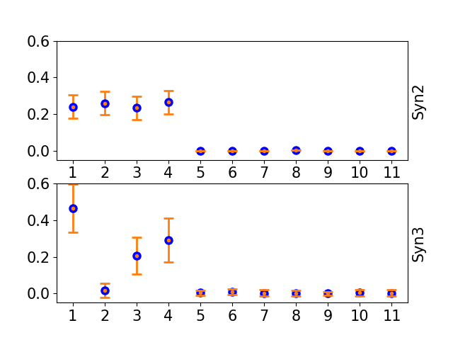
In the experiment featuring synthetic datasets, we also verify how well BIF can estimate the uncertainty of the importance values. While non-probabilitic methods provide only the point estimate, Bayesian approach allows to estimate how confident the algorithm is about its output, in this case, the feature importance value. Thus, Fig. 2 shows the posterior mean and variance of the importance vector. The posterior variance stands for the confidence the BIF algorithm has about the learned feature importance. Fig. 2 shows the variance of two datasets, Syn2 which is easier and Syn3 which is harder to predict its label. BIF consequently indicates the higher uncertainty for the harder dataset and lower for the easier dataset. This information can be particularly helpful when assessing the confidence about the importance of each feature, for example, it answers the question how probable it is that a given feature is the most important.
Discussion.
In selecting feature selection method, it is worth considering their advantages and disadvantages. The BIF global is a method whose number of parameters is linear in the number of features, however it works only in the global setting. The local variants require an additional network which may however work better, also in the global setting (by averaging the importance over all the data points). In terms of performance, the sampling and point estimate BIF produce similar results, however the shortcoming of the point estimate is that it produces the results with relatively high variance (see Supplementary materials for summary results). On the other hand, sampling is more time-consuming due to evaluations required for each sample. It is also worth discussing the effect of features on the label in synthetic datasets. In particular, Syn1 and Syn2 datasets affect the label positively, while in Syn3 we deal with a sine term which may affect the label both positively and negatively. Despite that, the feature has been detected successfully to large extent. Nonetheless, Syn3 is the most challenging dataset among the three synthetic global datasets.
| Adult | Credit | Intrusion | ||||||||
|---|---|---|---|---|---|---|---|---|---|---|
| 1 | 3 | 5 | 1 | 3 | 5 | 1 | 3 | 5 | ||
| Local | BIF | 80.0 | 81.8 | 82,3 | 90.5 | 92.9 | 94.1 | 81.6 | 95.8 | 83.6 |
| L2X | 78.6 | 81.7 | 83.1 | 86.5 | 89.1 | 92.8 | 81.9 | 79.0 | 77.4 | |
| INVASE | 73.5 | 78.6 | 82.1 | 81.4 | 90.9 | 91.5 | 70.5 | 76.6 | 45.5 | |
| SHAP | 71.8 | 74.8 | 76.9 | 86.8 | 84.9 | 84.5 | 69.1 | 72.6 | 73.4 | |
| LIME | 77.6 | 78.9 | 80.6 | 85.2 | 87.3 | 94.3 | 78.0 | 89.5 | 83.8 | |
| Global | BIF | 78.2 | 76.5 | 82.4 | 96.1 | 94.9 | 94.9 | 82.3 | 82.4 | 82.6 |
| L2X | 65.5 | 77.2 | 80 | 82.6 | 92.2 | 95.2 | 39.3 | 59.9 | 81.1 | |
| INVASE | 65.5 | 82.3 | 82.4 | 95.5 | 90.7 | 94.6 | 44.3 | 82.3 | 82.3 | |
| SHAP | 76.6 | 79.7 | 83.1 | 96.1 | 94.3 | 96.4 | 82.3 | 87.1 | 87.1 | |
| LIME | 77.6 | 78.9 | 75.9 | 92.4 | 88.9 | 92.5 | 82.3 | 81.3 | 83.4 |
5.2 Real-world data
Tabular Data
We consider credit (Cre) (license: DbCL v1.0) and adult (Dua and Graff 2017) datasets with tabular input features and binary labels, and intrusion (Int) dataset with multi-class labels. Adult dataset predicts whether income exceeds $50K a year based on census data, credit dataset classifies applicants for credit availability, and the intrusion dataset classifies several types of burglaries.
This experiment consists of two parts. In the first part, we look for globally important features in the entire dataset. In the second part,we perform local feature search. As there is no known ground truth about the features, we evaluate the effectiveness of each method by selecting top features which are deemed most significant, and then performing the post-hoc classification task given these input features with removing the rest. In the global setting, features are fixed for the entire dataset, while in the local setting each sample can select a different set of features. In the experiments, we standardize each feature to have a zero mean to mitigate the issue of out-of-distribution examples which could occur in the case of non-zero mean real-world features.
BIF outputs a probability distribution which directly allows to identify top features. On the other hand, INVASE and L2X output binary decisions for feature importance. For global explanations, we average the output for all data points, thus creating global ranking of features in INVASE and L2X. For local explanations, in case of L2X we can specify relevant features. INVASE has no such option and thus, for the fairest comparison, we use the selection probability given by the selector network as a proxy of importance score. In the global case of LIME, we average the rankings for the individual instances. As shown in Table 5 (classification accuracy averaged over five independent runs), BIF performs well in both tasks, with a bigger edge in global search. We found that local explanation search is significantly more challenging than the global one, reflected in the lower classification accuracy. And so although the results provide good insight into which features are important locally, one should proceed with caution when relying on a subset of local features, especially in more risk-averse applications.
Please also note that as we use a separate validation set to test the top features, increasing the number of features may have a contrary effect and actually decrease the test accuracy. This happens irrelevant of the method, likely due to correlation between features and the nature of the model .
MNIST Data.
Following (Chen et al. 2018), we construct a dataset with two labels by gathering the 3 and 8 digit samples from MNIST (LeCun et al. 2010) (license: CC BY-SA 3.0). We then train BIF, as well as L2X and INVASE models to select 4x4 pixel patches as relevant features. As the inputs have a dimensionality of 28x28, there are 49 features to choose from. To evaluate the quality of the selection, we first mask the test set by setting all non-selected patches to 0 and then use a classifier which was trained on unmasked data to compute the post-hoc accuracy on this modified test set. The post-hoc accuracies averaged over 5 runs are shown in Fig. 3a for different numbers of selected features.
| BIF | 0.788 | 0.937 | 0.973 | 0.98 | 0.981 |
| L2X | 0.633 | 0.761 | 0.84 | 0.871 | 0.864 |
| INVASE | 0.584 | 0.78 | 0.901 | 0.915 | 0.905 |
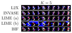
The selection method differs between models. For BIF, we select the most highly weighted patches and for L2X, is set in advance. INVASE is treated differently, as the number of selected features varies and can only be modified implicitly through the strength of the regularizer. So we tune the regularizer strength to different values such that the average number of selected features equals . The values we use are 100, 50, 23, 18.5 and 15.5 for . We also show the qualitative results of each method in Fig. 3b.
5.3 Divergence for comparing feature importance distributions.
As described in Sec. 4, our method outputs the parameters of the Dirichlet distribution over the feature importance. With the deliberate choice of Dirichlet distribution, we can obtain a closed-form distance metric such as the KL divergence between two BIF’s learned Dirichlet distributions. We exploit this to study trade-offs between important notions such as explainability, privacy, and fairness. In particular, we apply the KL-divergence to describe the level of explainability sacrificed at the cost of increase in privacy of a classifier. We show a similar experiment for the fairness trade-off in the supplementary materials.
We use the Diabetes Readmisison dataset44 4 We followed the data pre-processing given in https://www.kaggle.com/victoralcimed/diabetes-readmission-through-logistic-regression (Rizvi et al. 2014) (license: CC0 1.0) to train a private classifier. We consider a private classifier using the differentially private stochastic gradient descent (DP-SGD) technique (Abadi et al. 2016), which perturbs the gradients during training to yield a classifier that guarantees a certain level of privacy, that is, it ensures that we cannot recreate the data that the model has been trained on. Fig. 4 (Left) shows how the classifier loses the accuracy measured in terms of the area under the curve as we increase the privacy level. Different privacy levels introduce different levels of noise we induced to the gradients during training (the higher , the smaller the noise level, and corresponds to the non-private classifier). As the loss of accuracy is a known phenomenon, we aim to show a different effect, namely the impact of noise on the possibility to explain the data in form of the difference between the feature distribution without the noise and that when the noise is present at different levels.


The experiment shows two things. Firstly, as Fig. 4 and the KL divergence chart of Fig. 5 demonstrate, the relative differences in importance between features decrease as we increase the levels of noise. BIF-tuned probabilities well reflect the intuition that as we increase privacy levels, the explainability in form of assessing the correct distribution of feature importance decreases. In the Supplementary material, we also include the analysis regarding the INVASE, which shows that this intuition may not be exactly reflected in how features are selected. Secondly as Fig. 5 shows, even though the relative differences may be obfuscated by the noise, even at high levels of privacy we may distinguish the most relevant features, showing robustness of the feature selection ranking to the noise.
6 Conclusion
Our novel Bayesian perspective yielded the framework that is accurate and also provides confidence about the feature importance both in global and local settings. The learnt distributions over features can be useful to measure explainability in a variety of applications.
Appendix A Experiment details for synthetic data
Below we give details on the experimental setups for each of the results presented in the paper.
A.1 Methods
BIF.
We first train the network for 500 epochs. Then we freeze these weights and finetune the switch vector or switch network for 10 epochs. In the experiment 1 we use analytic mean of Dirichlet distribution. We also tested the sampling but analytic mean proved to work faster and better.
L2X.
We load the additional datasets for 125 epochs (preserving number iterations due to the smaller dataset). On Syn4 and Syn5 where the number of relevant features is not fixed, we report results for k=5, which maximized .
INVASE.
We run the original code for 10k iterations. As suggested by the authors (https://github.com/jsyoon0823/INVASE/issues/1), we set for Syn5 and to otherwise. We use SELU nonlinearities for Syn4-6 but not for Syn3, as we obtained better results with ReLUs on the first three datasets.
A.2 Standard deviation comparison.
We compare here the standard deviation of the selected methods used in the main text.
| Syn 1 | Syn 2 | Syn 3 | Syn 4 | Syn 5 | Syn 6 | |
|---|---|---|---|---|---|---|
| BIF (inst, samp) | 0 | 0 | 0.107 | 0.019 | 0.010 | 0.025 |
| BIF (inst, pe) | 0 | 0 | 0.201 | 0.015 | 0.061 | 0.093 |
| BIF (gl, samp) | 0 | 0 | 0.201 | NA | NA | NA |
| BIF | |||||
|---|---|---|---|---|---|
| L2X | |||||
| INVASE |
Appendix B Experiment details for real-world data
B.1 Tabular data information
BIF.
We perform experiments on three real-world tabular datasets, adult, credit and intrusion. We included more details about these datasets and experimental details below. In these experiments we use the point estimate without KL-regularizer.
Credit
Credit card fraud detection dataset contains the categorized information of credit card transactions which were either fraudelent or not. Ten dataset comes from a Kaggle competition and is available at the source, https://www.kaggle.com/mlg-ulb/creditcardfraud. The original data has 284807 examples, of which negative samples are 284315 and positive 492. The dataset has 31 categories, 30 numerical features and a binary label. We used all but the first feature (Time).
Adult
The dataset contains information about people’s attributes and their respective income which has been thresholded and binarized. It has 22561 examples, and 14 features and a binary label. The dataset can be downloaded by means of SDGym package,https://pypi.org/project/sdgym/.
Intrusion
The dataset was used for The Third International Knowledge Discovery and Data Mining Tools Competition held at the Conference on Knowledge Discovery and Data Mining, 1999, and can be found at http://kdd.ics.uci.edu/databases/kddcup99/kddcup99.html. We used the file, kddcup.data_10_percent.gz. It is a multi-class dataset with five labels describing different types of connection intrusions. The labels were first grouped into five categories and due to few examples, we restricted the data to the top four categories.
B.2 Standard deviation information for Table 2
| Adult | Credit | Intrusion | |||||||
|---|---|---|---|---|---|---|---|---|---|
| 1 | 3 | 5 | 1 | 3 | 5 | 1 | 3 | 5 | |
| BIF (Local) | 1.547 | 0.581 | 0.655 | 3.804 | 1.217 | 2.737 | 2.269 | 8.874 | 3.926 |
| BIF (Global) | 1.220 | 5.88 | 0.000 | 1.579 | 0.839 | 0.200 | 4.712 | 6.133 | 3.128 |
B.3 MNIST data
We generate the binary classification dataset by selecting all samples of classes 3 and 8 from MNIST, keeping the separExperimentracy on the feature-selected data. In all cases below, the feature selection models output 49 dimensions representing the patches, which are then copied over 4x4 pixel patches to a full output size of 784.
BIF.
We first train a classifier for 10 epochs with the same architecture as the post-hoc accuracy model, but without batch-norm, as this leads to more stable selector training. Following this, the selector is network is trained for 10 epochs and then we use the selector to generate feature importances for the full test-set. For each sample the most highly weighted patches are kept and the remaining features are set to 0.
L2X.
Because the original released L2X code does not contain the setup for the MNIST experiment, we use our own implementation based on the released code for synthetic data. We increase hidden dimensions in the selector and classifier parts of the model from & to & due to the higher data complexity.
INVASE.
We adapt the INVASE setup for synthetic data to mnist and tune the parameter in order to produce feature selections with different average numbers of selected features. For ranging from 1 to 5, we use values of 100, 50, 23, 18.5, 15.5. As the relationship between the value of and average is not reliable, we discard results from random seeds that didn’t produce the desired . The chosen random seeds are listed in the experiment code.
Appendix C Importance value estimates short analysis
In the paper, we mention that BIF’s importance values are more accurate due than those from the existing literature, that is we look here not whether an input feature is important but how important it is. Here we briefly elaborate on this statement and provide some examples. This sort of analysis can be done on synthetic datasets (Syn 1-3) where we know the ground truth and know how the features were generates. Thus, Syn1 and Syn2 are the datasets where the weight of each of the important feature is equal and so we would expect each relevant weight to be equal. In fact, this is what we see in the output of BIF. The global weights for Syn1 are and for Syn2 are , both of which very closely discover the weight importance. Furthermore, we provide below a comparison example with the other methods for a more challenging Syn3.
Appendix D Privacy trade-off analysis for INVASE

For INVASE (Yoon et al. 2018), we adjust the setup so that we jointly train the baseline network with a private classifier, then freeze the baseline network, and only update the selector and predictor networks. As INVASE is a method for instance-wise feature selection, once trained, we use INVASE to output the feature selection for the test datapoints, and average the selection probability (the Bernoulli distribution over the feature selection) across those test datapoints.
The Middle and Right plots in Fig. 7 compare INVASE and BIF. In the case of INVASE, the KL divergence is not necessarily informative. The divergence metric between the selection distribution under the non-private classifier and that at different privacy level differ, while the selected features remains similar.
Right: While KL divergence shows a similar pattern as the middle plot, the difference in the KL divergence under INVASE lacks consistency with the learned importance of features (selected features by INVASE are written in Orange). For instance, at and , INVASE selected no features as important. On the other hand, at and INVASE selected the number of inpatient as an important feature.
Appendix E Fainess trade-off analysis
Fairness vs feature importance. First, we show the usefulness of our method to study the trade-off between explainability in terms of feature importance and fairness. We consider a fair classifier introduced in (Tonk 27 April, 2018), and the Adult data to train a fair classifier in terms of Race. For this experiment, we modify the dataset, such that it only consists of features by excluding the Race and Sex features as done in (Tonk 27 April, 2018). As shown in (1) in Fig. 8, the classifier loses accuracy measured in terms of the area under the curve as we increase the fairness measured in terms of the percentage rule (Tonk 27 April, 2018), which is a well-known phenomenon, but we aim to show that BIF allows to measure well the loss in explainability when increasing the fairness of the classifier.
In this case, as shown in (2) and (3) of Fig. 8, both INVASE and BIF demonstrate gradual loss of explainability as the KL divergence between the feature distribution under the classifier trained without any fairness constraint and that at different levels of fairness ( and fair) increases as the fairness constraint increases. However, the vanilla INVASE by outputting just a set of important features does not distinguish between the level of and (by outputting for both levels). Meanwhile, under BIF, the difference in the KL divergence is well reflected in the learned importance as shown in (4). By virtue of assigning continuous importance weights, BIF is able to account for smaller changes in the trained model than a discrete method like INVASE.
Appendix F Experiment details for Trade-offs
F.1 Feature importance vs fairness
Dataset
We use the Adult data used in the earlier section, with a change of excluding sex and race from the input features. The resulting dataset has input features: age(0), workclass(1), fnlwgt(2), education(3), education number (4), marital status(5), occupation(6), relationship(7), capital gain(8), capital loss(9), hours per week(10), native country(11).
Fair classifiers
We use this modified dataset and train a classifier with different fairness constraints following code from https://github.com/equialgo/fairness-in-ml/blob/master/fairness-in-ml.ipynb
BIF
Given a classifier at each level of fairness, in terms of percentage rule based on race, we learn the global feature importance vector for epochs. When computing the variational lower bound, we used a single sample. We set the prior parameter to be . As shown in the main text, initially when the classifier is unfair, the marital status(5) is the most important, and the education number (4) is in the second place, and the capital gain (8) is in the third place. As we increase the fairness in training the classifier, while the importance of marital status remains almost the same, the education number and capital gain become less important, while the age starts appearing to be important.
INVASE
We train the INVASE model by exchanging the classifier component with the pre-trained fair models and only optimize the selector component. This diverges from the standard way of training INVASE, but despite the frozen classifier the model achieves an accuracy of 83% by the end of training.
F.2 Feature importance vs privacy
Dataset
We use the original Adult dataset, which contains input features: age(0), workclass(1), fnlwgt(2), education(3), education number (4), marital status(5), occupation(6), relationship(7), race(8), sex(9), capital gain(10), capital loss(11), hours per week(12), native country(13).
Private classifiers
Using this dataset, we train a classifier, a 3-layer feedforward network with and hidden units in each hidden layer for epochs, using the differentially private stochastic gradient descent (DP-SGD), which adds appropriately adjusted amount of noise to the gradient during training for privacy. The amount of noise and the corresponding privacy guarantee of the classifier is summarized in Table 6. The highly nonlinear relationship between the noise level and the corresponding privacy level is calculated by using the autodp package: https://github.com/yuxiangw/autodp.
| noise level | privacy guarantee |
|---|---|
BIF
Under each of the classifier, we learn the global feature importance of the input features using BIF for epochs. When computing the variational lower bound, we used a single sample. We set the prior parameter to be . Under the non-private classifier, relationship(7) status is the most important, and education number (4) is second, and capital gain(10) is the third. As we increase the noise level for a stronger privacy guarantee, the importance of the relationship(7) feature gets lower and other features such as age(0) and marital status(5) become more important.
INVASE
The setup here equals the setup for fair models, with the difference that privacy classifier models are loaded instead.
Appendix G Matthews correlation coefficient
Matthews correlation coefficient that is used in the Experiments section of the main text is defined as follows:
Appendix H Hardware
We have implemented our experiments in PyTorch (Paszke et al. 2019) on a laptop with GeForce RTX 2080. In our experiments we also used Nvidia Kepler20 and Kepler80 GPUs, or a cluster consisting of five Tesla K80 and GeForce RTX 2080 Ti.
References
- (1) Kaggle credit card fraud detection dataset. URL https://www.kaggle.com/mlg-ulb/creditcardfraud?select=creditcard.csv.
- (2) Kdd cup 1999 data, intrusion dataset. URL http://kdd.ics.uci.edu/databases/kddcup99/kddcup99.html.
- Abadi et al. (2016) M. Abadi, A. Chu, I. Goodfellow, H. Brendan McMahan, I. Mironov, K. Talwar, and L. Zhang. Deep learning with differential privacy. ArXiv e-prints, July 2016.
- Ancona et al. (2017) Marco Ancona, Enea Ceolini, A. Cengiz Öztireli, and Markus H. Gross. A unified view of gradient-based attribution methods for deep neural networks. CoRR, abs/1711.06104, 2017. URL http://arxiv.org/abs/1711.06104.
- Candes et al. (2016) Emmanuel Candes, Yingying Fan, Lucas Janson, and Jinchi Lv. Panning for gold: Model-free knockoffs for high-dimensional controlled variable selection. Journal of the Royal Statistical Society: Series B (Statistical Methodology), 80, 10 2016. doi: 10.1111/rssb.12265.
- Charnes et al. (1988) A. Charnes, B. Golany, M. Keane, and J. Rousseau. Extremal principle solutions of games in characteristic function form: Core, chebychev and shapley value generalizations. 1988.
- Chen et al. (2018) Jianbo Chen, Le Song, Martin J Wainwright, and Michael I Jordan. Learning to explain: An information-theoretic perspective on model interpretation. arXiv preprint arXiv:1802.07814, 2018.
- Dua and Graff (2017) Dheeru Dua and Casey Graff. UCI machine learning repository, adult dataset, 2017. URL https://archive.ics.uci.edu/ml/datasets/adult.
- Goodman and Flaxman (2016) Bryce Goodman and Seth Flaxman. European Union regulations on algorithmic decision-making and a “right to explanation”. arXiv e-prints, art. arXiv:1606.08813, Jun 2016.
- Guyon and Elisseeff (2003) Isabelle Guyon and André Elisseeff. An introduction to variable and feature selection. J. Mach. Learn. Res., 3(null):1157–1182, March 2003. ISSN 1532-4435.
- Hall (1999) Mark A. Hall. Correlation-based feature selection for machine learning. Technical report, 1999.
- Hanchuan Peng et al. (2005) Hanchuan Peng, Fuhui Long, and C. Ding. Feature selection based on mutual information criteria of max-dependency, max-relevance, and min-redundancy. IEEE Transactions on Pattern Analysis and Machine Intelligence, 27(8):1226–1238, 2005.
- Kira and Rendell (1992) Kenji Kira and Larry A. Rendell. A practical approach to feature selection. In Derek Sleeman and Peter Edwards, editors, Machine Learning Proceedings 1992, pages 249 – 256. Morgan Kaufmann, San Francisco (CA), 1992. ISBN 978-1-55860-247-2.
- Knowles (2015) David A. Knowles. Stochastic gradient variational Bayes for gamma approximating distributions. arXiv e-prints, art. arXiv:1509.01631, Sep 2015.
- Kuhn et al. (2013) Max Kuhn, Kjell Johnson, et al. Applied predictive modeling, volume 26. Springer, 2013.
- LeCun et al. (2010) Yann LeCun, Corinna Cortes, and CJ Burges. Mnist handwritten digit database. ATT Labs [Online]. Available: http://yann.lecun.com/exdb/mnist, 2, 2010.
- Linardatos et al. (2021) Pantelis Linardatos, Vasilis Papastefanopoulos, and Sotiris Kotsiantis. Explainable ai: A review of machine learning interpretability methods. Entropy, 23(1), 2021. ISSN 1099-4300. doi: 10.3390/e23010018. URL https://www.mdpi.com/1099-4300/23/1/18.
- Lundberg and Lee (2017a) Scott Lundberg and Su-In Lee. A unified approach to interpreting model predictions. arXiv preprint arXiv:1705.07874, 2017a.
- Lundberg and Lee (2017b) Scott M Lundberg and Su-In Lee. A unified approach to interpreting model predictions. In I. Guyon, U. V. Luxburg, S. Bengio, H. Wallach, R. Fergus, S. Vishwanathan, and R. Garnett, editors, Advances in Neural Information Processing Systems 30, pages 4765–4774. Curran Associates, Inc., 2017b.
- Matthews (1975) Brian W. Matthews. Comparison of the predicted and observed secondary structure of t4 phage lysozyme. Biochimica et Biophysica Acta (BBA) - Protein Structure Volume 405, Issue 2, 1975.
- Paszke et al. (2019) Adam Paszke, Sam Gross, Francisco Massa, Adam Lerer, James Bradbury, Gregory Chanan, Trevor Killeen, Zeming Lin, Natalia Gimelshein, Luca Antiga, Alban Desmaison, Andreas Kopf, Edward Yang, Zachary DeVito, Martin Raison, Alykhan Tejani, Sasank Chilamkurthy, Benoit Steiner, Lu Fang, Junjie Bai, and Soumith Chintala. Pytorch: An imperative style, high-performance deep learning library. In H. Wallach, H. Larochelle, A. Beygelzimer, F. d'Alché-Buc, E. Fox, and R. Garnett, editors, Advances in Neural Information Processing Systems 32, pages 8024–8035. Curran Associates, Inc., 2019. URL http://papers.neurips.cc/paper/9015-pytorch-an-imperative-style-high-performance-deep-learning-library.pdf.
- Ribeiro et al. (2016a) Marco Tulio Ribeiro, Sameer Singh, and Carlos Guestrin. Why should I trust you?: Explaining the predictions of any classifier. Proceedings of the 22nd ACM SIGKDD International Conference on Knowledge Discovery and Data Mining, 2016a.
- Ribeiro et al. (2016b) Marco Tulio Ribeiro, Sameer Singh, and Carlos Guestrin. Why should i trust you?: Explaining the predictions of any classifier. In Proceedings of the 22nd ACM SIGKDD international conference on knowledge discovery and data mining, pages 1135–1144. ACM, 2016b.
- Rizvi et al. (2014) Ali Rizvi, John N. Clore, Krzysztof J. Cios, Sebastian Ventura, Juan L. Olmo, Chris Gennings, Jonathan P. DeShazo, and Beata Strack. Impact of hba1c measurement on hospital readmission rates: Analysis of 70,000 clinical database patient records. Apr 2014. URL https://doi.org/10.1155/2014/781670.
- Shrikumar et al. (2017) Avanti Shrikumar, Peyton Greenside, and Anshul Kundaje. Learning important features through propagating activation differences. In Proceedings of the 34th International Conference on Machine Learning - Volume 70, ICML’17, page 3145–3153. JMLR.org, 2017.
- Smilkov et al. (2017) Daniel Smilkov, Nikhil Thorat, Been Kim, Fernanda B. Viégas, and Martin Wattenberg. Smoothgrad: removing noise by adding noise. CoRR, abs/1706.03825, 2017. URL http://arxiv.org/abs/1706.03825.
- Sundararajan et al. (2017) Mukund Sundararajan, Ankur Taly, and Qiqi Yan. Axiomatic attribution for deep networks. CoRR, abs/1703.01365, 2017. URL http://arxiv.org/abs/1703.01365.
- Tibshirani (1996) R. Tibshirani. Regression shrinkage and selection via the lasso. Journal of the Royal Statistical Society (Series B), 58:267–288, 1996.
- Tonk (27 April, 2018) Stijn Tonk. Towards fairness in ML with adversarial networks, 27 April, 2018. URL https://godatadriven.com/blog/towards-fairness-in-ml-with-adversarial-networks/.
- Voigt and Bussche (2017) Paul Voigt and Axel von dem Bussche. The EU General Data Protection Regulation (GDPR): A Practical Guide. Springer Publishing Company, Incorporated, 1st edition, 2017. ISBN 3319579584, 9783319579580.
- Yoon et al. (2018) Jinsung Yoon, James Jordon, and Mihaela van der Schaar. Invase: Instance-wise variable selection using neural networks. 2018.