跳到论文正文
W Papers独立论文阅读器 arXiv:2010.13798 论文正文 计算阅读时间 · 0%
引用这篇论文根据当前论文元数据生成,正式投稿前建议核对。


License: arXiv.org perpetual non-exclusive license
arXiv:2010.13798v2 [hep-th] 21 Apr 2021

TUM-HEP 1288/20

Eclectic flavor scheme from ten-dimensional string theory - II
Detailed technical analysis

Hans Peter Nillesa, Saúl Ramos–Sánchezb, Patrick K.S. Vaudrevangec

aBethe Center for Theoretical Physics and Physikalisches Institut der Universität Bonn,
Nussallee 12, 53115 Bonn, Germany

bInstituto de Física, Universidad Nacional Autónoma de México,
POB 20-364, Cd.Mx. 01000, México

cPhysik Department T75, Technische Universität München,
James-Franck-Straße 1, 85748 Garching, Germany

String theory leads to a flavor scheme where modular symmetries play a crucial role. Together with the traditional flavor symmetries they combine to an eclectic flavor group, which we determine via outer automorphisms of the Narain space group. Unbroken flavor symmetries are subgroups of this eclectic group and their size depends on the location in moduli space. This mechanism of local flavor unification allows a different flavor structure for different sectors of the theory (such as quarks and leptons) and also explains the spontaneous breakdown of flavor- and 𝒞​𝒫\mathcal{CP}-symmetries (via a motion in moduli space). We derive the modular groups, including 𝒞​𝒫\mathcal{CP} and RR-symmetries, for different sub-sectors of six-dimensional string compactifications and determine the general properties of the allowed flavor groups from this top-down perspective. It leads to a very predictive flavor scheme that should be confronted with the variety of existing bottom-up constructions of flavor symmetry in order to clarify which of them could have a consistent top-down completion.

1 Introduction

The consideration of finite modular flavor groups has been suggested in the pioneering work of Feruglio [1]. A combination of these modular symmetries and traditional flavor symmetries leads to the eclectic flavor scheme [2, 3]. Here, we present a study of the eclectic flavor approach towards ten-dimensional string theory with D=6D=6 compactified spatial dimensions11 1 For further work on modular flavor symmetries in string theory, see e.g. refs. [4, 5, 6, 7, 8, 9, 10, 11]. This generalizes previous work with D=2D=2 compact dimensions which is shown to fail to capture all the relevant properties of the eclectic picture. A few of the highlights of this discussion have been presented in an earlier paper [12] without explaining the full technical details. These highlights include

  • •

    a further enhancement of the eclectic group,

  • •

    a new interpretation of discrete RR-symmetries originating from modular transformations of the complex structure modulus,

  • •

    a relation between the RR-charges and the modular weights of matter fields, and

  • •

    new insights in the nature of 𝒞​𝒫\mathcal{CP}-symmetry and its spontaneous breakdown.

These results have been illustrated previously [3, 12] in an example of a D=2D=2 sublattice based on the 𝕋2/ℤ3\mathbbm{T}^{2}/\mathbbm{Z}_{3} orbifold. Here we shall now present the complete results in the generic situation and provide the full technical details of the derivation. In addition, we shall illustrate an interesting novel feature: the existence of accidental continuous (gauge) symmetries of the effective theory at special loci in moduli space, which turn out to be further enhancements of the traditional flavor symmetries.

In section 2 we shall discuss basic background material concerning the D=2D=2 Narain lattice formulation [13, 14, 15, 16] and its outer automorphisms relevant for (discrete) modular symmetries [17, 18]. These include the groups SL​(2,ℤ)T\mathrm{SL}(2,\mathbbm{Z})_{T} and SL​(2,ℤ)U\mathrm{SL}(2,\mathbbm{Z})_{U} for the Kähler modulus TT and the complex structure modulus UU, respectively, mirror symmetry as well as a 𝒞​𝒫\mathcal{CP}-like transformation. Results for the generators are summarized in table 1 for various 𝕋2/ℤK\mathbbm{T}^{2}/\mathbbm{Z}_{K} orbifolds. We include a discussion of the modular properties of the superpotential and Kähler potential in the modular invariant field theory, including modular weights and automorphy factors.

Section 3 concentrates on the discussion of those aspects of the modular group SL​(2,ℤ)U\mathrm{SL}(2,\mathbbm{Z})_{U} of the complex structure modulus which will become relevant for the analysis in D=6D=6 compact dimensions. In contrast to SL​(2,ℤ)T\mathrm{SL}(2,\mathbbm{Z})_{T} (which exchanges windings and momenta), SL​(2,ℤ)U\mathrm{SL}(2,\mathbbm{Z})_{U} can be given a fully geometrical interpretation. In previous discussions of D=2D=2 orbifolds 𝕋2/ℤK\mathbbm{T}^{2}/\mathbbm{Z}_{K}, the subtleties of this analysis have not yet been completely considered, because the modulus UU is frozen as a result of the orbifold twist (except for the case 𝕋2/ℤ2\mathbbm{T}^{2}/\mathbbm{Z}_{2} which has been discussed elsewhere [19]). We show here that, even with a frozen value ⟨U⟩\langle U\rangle of the complex structure UU, there are nontrivial elements of SL​(2,ℤ)U\mathrm{SL}(2,\mathbbm{Z})_{U} that remain unbroken. These lead to additional discrete RR-symmetries according to the stabilizer subgroups given in formula (82). These symmetries will be relevant for the D=6D=6 case in the form of sublattice rotations.

In section 4, we consider the 𝕋6/P\mathbbm{T}^{6}/P orbifold (with point group PP). We start with the discussion in full generality (including the restrictions of 𝒩=1\mathcal{N}=1 supersymmetry in four space-time dimensions) and then illustrate the results for the ℤ6\mathbbm{Z}_{6}-II orbifold. We shall identify the sublattice rotations of SL​(2,ℤ)U\mathrm{SL}(2,\mathbbm{Z})_{U}, their action on matter fields and determine which (fractional) modular weights are relevant for the emerging RR-symmetries. Section 4.3 includes a discussion of 𝒞​𝒫\mathcal{CP}-transformations, including the full D=6D=6 picture (summarized in table 3).

Section 5 presents the complete description for a sublattice 𝕋2/ℤ3\mathbbm{T}^{2}/\mathbbm{Z}_{3} of the ℤ6\mathbbm{Z}_{6}-II orbifold. This includes the traditional flavor symmetry Δ⁡(54)\Delta(54), the finite modular symmetry T′T^{\prime} from SL​(2,ℤ)T\mathrm{SL}(2,\mathbbm{Z})_{T}, a discrete RR-symmetry ℤ9R\mathbbm{Z}_{9}^{R} from SL​(2,ℤ)U\mathrm{SL}(2,\mathbbm{Z})_{U} as well as a 𝒞​𝒫\mathcal{CP}-like transformation (which is separately discussed in subsections 5.6 and 5.7). The maximal eclectic group is shown to have 3,8883,888 elements, extending Ω⁡(2)≅[1944,3448]\Omega(2)\cong[1944,3448] (see table 5) by the 𝒞​𝒫\mathcal{CP}-like transformation. We discuss restrictions of this symmetry on the form of the superpotential and Kähler potential of the 𝒩=1\mathcal{N}=1 supersymmetric field theory.

Only part of the eclectic flavor symmetry is realized linearly. For generic values of the moduli only the traditional flavor symmetry is unbroken. This symmetry will be enhanced at special points (or sub-loci) of the moduli space. In section 6 we present this phenomenon of local flavor unification for the 𝕋2/ℤ3\mathbbm{T}^{2}/\mathbbm{Z}_{3} orbifold and identify these enhanced groups (see table 6 and figure 3) as well as the specific forms of the superpotential. Moving away from these sub-loci in moduli space will correspond to a spontaneous breakdown of the enhanced flavor groups (in particular also for the violation of 𝒞​𝒫\mathcal{CP}-symmetry). A novel observation concerns the emergence of (accidental) continuous gauge symmetries at special loci in moduli space, here discussed in section 6.4.

Section 7 will present conclusions and an outlook for future applications of our results.

Note to the reader: As our discussion is partially very technical we include a short specific summary at the end of each section 2–6 to make the results of the discussion as transparent as possible.

2 Modular symmetries in string theory

In general, the modular group SL⁡(2,ℤ)\mathrm{SL}(2,\mathbbm{Z}) can be defined as the group generated by two abstract generators, S\mathrm{S} and T\mathrm{T}, that satisfy the defining relations

S4=(S​T)3=𝟙andS2​T=T​S2.\mathrm{S}^{4}~=~(\mathrm{S}\,\mathrm{T})^{3}~=~\mathbbm{1}\qquad\mathrm{and}\qquad\mathrm{S}^{2}\,\mathrm{T}~=~\mathrm{T}\,\mathrm{S}^{2}\;. (1)

It turns out convenient to represent these generators by the matrices

S:=(01−10)andT:=(1101).\mathrm{S}~:=~\left(\begin{array}[]{cc}0&1\\ -1&0\end{array}\right)\qquad\mathrm{and}\qquad\mathrm{T}~:=~\left(\begin{array}[]{cc}1&1\\ 0&1\end{array}\right)\;. (2)

In this context, the elements γ∈SL⁡(2,ℤ)\gamma\in\mathrm{SL}(2,\mathbbm{Z}) can be expressed by 2×22\times 2 matrices with integer entries and determinant one, i.e.

γ:=(abcd),witha​d−b​c=1,a,b,c,d∈ℤ.\gamma~:=~\left(\begin{array}[]{cc}a&b\\ c&d\end{array}\right)\,,\qquad\mathrm{with}\qquad ad-bc=1,\,a,b,c,d\in\mathbbm{Z}\;. (3)

Particularly relevant in string models (and in bottom-up flavor model building) are the so-called finite modular groups. Their generators are also denoted by S\mathrm{S} and T\mathrm{T}, which fulfill the following defining relations

ΓN′:\displaystyle\Gamma^{\prime}_{N}~: S4=(S​T)3=TN=𝟙andS2​T=T​S2,\displaystyle~\mathrm{S}^{4}~=~(\mathrm{S}\,\mathrm{T})^{3}~=~\mathrm{T}^{N}~=~\mathbbm{1}\qquad\mathrm{and}\qquad\mathrm{S}^{2}\,\mathrm{T}~=~\mathrm{T}\,\mathrm{S}^{2}\;, (4a)
ΓN:\displaystyle\Gamma_{N}~: S2=(S​T)3=TN=𝟙,\displaystyle~\mathrm{S}^{2}~=~(\mathrm{S}\,\mathrm{T})^{3}~=~\mathrm{T}^{N}~=~\mathbbm{1}\;, (4b)

where ΓN′\Gamma^{\prime}_{N} is the double cover of ΓN\Gamma_{N}. The finite modular groups ΓN′\Gamma^{\prime}_{N} and ΓN\Gamma_{N} can be obtained from the modular groups SL⁡(2,ℤ)\mathrm{SL}(2,\mathbbm{Z}) and PSL⁡(2,ℤ)≅SL⁡(2,ℤ)/ℤ2\mathrm{PSL}(2,\mathbbm{Z})\cong\mathrm{SL}(2,\mathbbm{Z})/\mathbbm{Z}_{2} as the quotients ΓN′≅SL⁡(2,ℤ)/Γ⁡(N)\Gamma^{\prime}_{N}\cong\mathrm{SL}(2,\mathbbm{Z})/\Gamma(N) and ΓN≅PSL⁡(2,ℤ)/Γ~​(N)\Gamma_{N}\cong\mathrm{PSL}(2,\mathbbm{Z})/\tilde{\Gamma}(N), where Γ(N)≅⟨γ∈SL(2,ℤ)|γ=𝟙modN⟩\Gamma(N)\cong\left\langle\gamma\in\mathrm{SL}(2,\mathbbm{Z})\,|\,\gamma=\mathbbm{1}\mod{N}\right\rangle and Γ~(N)≅⟨γ∈PSL(2,ℤ)|γ=𝟙modN⟩\tilde{\Gamma}(N)\cong\left\langle\gamma\in\mathrm{PSL}(2,\mathbbm{Z})\,|\,\gamma=\mathbbm{1}\mod{N}\right\rangle are modular congruence subgroups.

2.1 Narain lattice of torus compactifications

In string theory, target-space modular symmetries can arise from the two-dimensional worldsheet CFT. To see this, let us first consider string theory compactified on a DD-dimensional torus 𝕋D\mathbbm{T}^{D}, which is most naturally described in the Narain formulation [13, 14, 15]. There, one considers right- and left-moving string coordinates yRy_{\mathrm{R}} and yLy_{\mathrm{L}}, which are related to the ordinary internal coordinates yy and their dual coordinates y~\tilde{y} via

y:=α′2​(yL+yR)andy~:=α′2​(yL−yR).y~:=~\sqrt{\frac{\alpha^{\prime}}{2}}\left(y_{\mathrm{L}}+y_{\mathrm{R}}\right)\qquad\mathrm{and}\qquad\tilde{y}~:=~\sqrt{\frac{\alpha^{\prime}}{2}}\left(y_{\mathrm{L}}-y_{\mathrm{R}}\right)\;. (5)

Then, (yR,yL)(y_{\mathrm{R}},y_{\mathrm{L}}) are compactified on a 2​D2D-dimensional auxiliary torus. This torus is defined by the so-called Narain lattice Γ\Gamma that is spanned by the so-called Narain vielbein EE. In more detail, the Narain torus boundary condition in this formalism reads

(yRyL)∼(yRyL)+λ,whereλ∈Γ:={E​N^|N^=(nm)∈ℤ2​D},\left(\begin{array}[]{c}y_{\mathrm{R}}\\ y_{\mathrm{L}}\end{array}\right)~\sim~\left(\begin{array}[]{c}y_{\mathrm{R}}\\ y_{\mathrm{L}}\end{array}\right)+\lambda\;,\quad\mathrm{where}\quad\lambda~\in~\Gamma~:=~\Bigg\{E\,\hat{N}~\Big|~\hat{N}=\left(\begin{array}[]{c}n\\ m\end{array}\right)~\in~\mathbbm{Z}^{2D}\Bigg\}\;, (6)

and n,m∈ℤDn,m\in\mathbbm{Z}^{D} are known as winding and Kaluza–Klein (KK) numbers, respectively. Due to worldsheet modular invariance of the one-loop string partition function, the Narain lattice Γ\Gamma spanned by EE has to be an even, integer, self-dual lattice with metric of signature (D,D)(D,D). This translates into the following condition on the Narain vielbein EE:

ET​η​E=η^:=(0𝟙D𝟙D0),whereη:=(−𝟙D00𝟙D)E^{\mathrm{T}}\eta\,E~=~\hat{\eta}~:=~\left(\begin{array}[]{cc}0&\mathbbm{1}_{D}\\ \mathbbm{1}_{D}&0\end{array}\right)\;,\quad\mathrm{where}\quad\eta~:=~\left(\begin{array}[]{cc}-\mathbbm{1}_{D}&0\\ 0&\mathbbm{1}_{D}\end{array}\right) (7)

denotes the metric of signature (D,D)(D,D) and 𝟙D\mathbbm{1}_{D} is the (D×D)(D\times D)-dimensional identity matrix. Then, the Narain scalar product of two Narain vectors λi=E​N^i∈Γ\lambda_{i}=E\,\hat{N}_{i}\in\Gamma with N^i=(ni,mi)∈ℤ2​D\hat{N}_{i}=(n_{i},m_{i})\in\mathbbm{Z}^{2D} for i∈{1,2}i\in\{1,2\} reads

λ1T​η​λ2=N^1T​η^​N^2=n1T​m2+m1T​n2∈ℤ.\lambda_{1}^{\mathrm{T}}\,\eta\,\lambda_{2}~=~\hat{N}_{1}^{\mathrm{T}}\hat{\eta}\,\hat{N}_{2}~=~n_{1}^{\mathrm{T}}m_{2}+m_{1}^{\mathrm{T}}n_{2}~\in~\mathbbm{Z}\;. (8)

This confirms that the lattice Γ\Gamma is integer and even, as the scalar product is integer and, if N^1=N^2\hat{N}_{1}=\hat{N}_{2}, even. Also, as expected from eq. (7), we note that η^\hat{\eta} is the Narain metric in the lattice basis.

In the absence of (discrete) Wilson lines [20], one can choose the (2​D×2​D)(2D\times 2D)-dimensional Narain vielbein EE fulfilling eq. (7) as

E:=12​(e−Tα′​(G−B)−α′​e−Te−Tα′​(G+B)α′​e−T),E~:=~\dfrac{1}{\sqrt{2}}\,\begin{pmatrix}\dfrac{e^{-\mathrm{T}}}{\sqrt{\alpha^{\prime}}}\,(G-B)&-\sqrt{\alpha^{\prime}}\,e^{-\mathrm{T}}\\[11.38092pt] \dfrac{e^{-\mathrm{T}}}{\sqrt{\alpha^{\prime}}}\,(G+B)&\phantom{-}\sqrt{\alpha^{\prime}}\,e^{-\mathrm{T}}\end{pmatrix}\;, (9)

see refs. [16, 17, 18]. Here, α′\alpha^{\prime} is the Regge slope that enters the Narain vielbein EE, such that EE is dimensionless. Then, EE is parameterized by the (D×D)(D\times D)-dimensional geometrical vielbein ee, yielding the metric G:=eT​eG:=e^{\mathrm{T}}e of the geometrical torus 𝕋D\mathbbm{T}^{D}, and the (D×D)(D\times D)-dimensional anti-symmetric BB-field BB.

Using the explicit parameterization (9), we can translate the Narain boundary condition (6) to the coordinates yy and their duals. We obtain

(yy~)∼(yy~)+(e​ne−T​(B​n+α′​m)).\left(\begin{array}[]{c}y\\ \tilde{y}\end{array}\right)~\sim~\left(\begin{array}[]{c}y\\ \tilde{y}\end{array}\right)\,+\,\left(\begin{array}[]{c}e\,n\\ e^{-\mathrm{T}}\,\left(B\,n+\alpha^{\prime}\,m\right)\end{array}\right)\;. (10)

Note that the boundary condition y∼y+e​ny\sim y+e\,n for the geometrical coordinates yy of closed strings motivates the name of n∈ℤDn\in\mathbbm{Z}^{D} as winding numbers of the geometrical torus 𝕋D\mathbbm{T}^{D} spanned by ee.

The Narain lattice Γ\Gamma is beneficial as it incorporates the winding numbers n∈ℤDn\in\mathbbm{Z}^{D} and the KK numbers m∈ℤDm\in\mathbbm{Z}^{D} on equal footing. Hence, it allows for a natural formulation of TT-duality in string theory, where KK and winding numbers get interchanged.

2.2 Outer automorphisms of the Narain lattice

In the Narain lattice basis, the Narain metric η^\hat{\eta} can be used to define the group of outer automorphisms22 2 Here, Oη^​(D,D,ℤ)\mathrm{O}_{\hat{\eta}}(D,D,\mathbbm{Z}) gives the discrete “rotational” outer automorphisms of the Narain lattice. Furthermore, there are continuous translations that act by conjugation on Narain lattice vectors and, therefore, correspond to the trivial automorphism of Γ\Gamma. of the Narain lattice Γ\Gamma that preserve the Narain metric η^\hat{\eta} as

Oη^(D,D,ℤ):=⟨Σ^|Σ^∈GL(2D,ℤ)withΣ^Tη^Σ^=η^⟩,\mathrm{O}_{\hat{\eta}}(D,D,\mathbbm{Z})~:=~\big\langle~\hat{\Sigma}~\big|~\hat{\Sigma}~\in~\mathrm{GL}(2D,\mathbbm{Z})\quad\mathrm{with}\quad\hat{\Sigma}^{\mathrm{T}}\hat{\eta}\,\hat{\Sigma}~=~\hat{\eta}~\big\rangle\;, (11)

such that each Narain lattice vector λ=E​N^∈Γ\lambda=E\,\hat{N}\in\Gamma is transformed by an outer automorphism Σ^∈Oη^​(D,D,ℤ)\hat{\Sigma}\in\mathrm{O}_{\hat{\eta}}(D,D,\mathbbm{Z}) according to

λ=E​N^⟶Σ^E​Σ^−1​N^∈Γ.\lambda=E\,\hat{N}~\stackrel{{\scriptstyle\hat{\Sigma}}}{{\longrightarrow}}~E\,\hat{\Sigma}^{-1}\hat{N}~\in~\Gamma\;. (12)

Here, we use Σ^−1\hat{\Sigma}^{-1} instead of Σ^\hat{\Sigma} for later convenience, see section 2.5. Then, Σ^−1​N^∈ℤ2​D\hat{\Sigma}^{-1}\hat{N}\in\mathbbm{Z}^{2D} and the Narain scalar product λT​η​λ\lambda^{\mathrm{T}}\,\eta\,\lambda from eq. (8) is invariant under the transformation (12). Note that the transformation of the Narain lattice vector eq. (12) can be interpreted as induced by the transformation of the Narain vielbein under outer automorphisms given by

E⟶Σ^E​Σ^−1forΣ^∈Oη^​(D,D,ℤ).E~\stackrel{{\scriptstyle\hat{\Sigma}}}{{\longrightarrow}}~E\,\hat{\Sigma}^{-1}\qquad\mathrm{for}\qquad\hat{\Sigma}~\in~\mathrm{O}_{\hat{\eta}}(D,D,\mathbbm{Z})\;. (13)

The group of outer automorphisms of the Narain lattice Oη^​(D,D,ℤ)\mathrm{O}_{\hat{\eta}}(D,D,\mathbbm{Z}) with these properties contains the modular group, as we discuss next.

For concreteness, let us focus on a geometrical two-torus 𝕋2\mathbbm{T}^{2} with D=2D=2. One can easily verify that Oη^​(2,2,ℤ)\mathrm{O}_{\hat{\eta}}(2,2,\mathbbm{Z}) contains two copies of SL⁡(2,ℤ)\mathrm{SL}(2,\mathbbm{Z}) as follows: First, we can define two Oη^​(2,2,ℤ)\mathrm{O}_{\hat{\eta}}(2,2,\mathbbm{Z}) elements

K^S:=(0−ϵ−ϵ0),K^T:=(𝟙20−ϵ𝟙2),whereϵ:=(01−10),\hat{K}_{\mathrm{S}}~:=~\left(\begin{array}[]{cc}0&-\epsilon\\ -\epsilon&0\end{array}\right)\quad,\quad\hat{K}_{\mathrm{T}}~:=~\left(\begin{array}[]{cc}\mathbbm{1}_{2}&0\\ -\epsilon&\mathbbm{1}_{2}\end{array}\right)\;,\quad\mathrm{where}\quad\epsilon~:=~\left(\begin{array}[]{cc}0&1\\ -1&0\end{array}\right)\;, (14)

which satisfy the defining relations (1) of SL⁡(2,ℤ)\mathrm{SL}(2,\mathbbm{Z}),

(K^S)4=(K^S​K^T)3=𝟙4and(K^S)2​K^T=K^T​(K^S)2.\left(\hat{K}_{\mathrm{S}}\right)^{4}~=~\left(\hat{K}_{\mathrm{S}}\,\hat{K}_{\mathrm{T}}\right)^{3}~=~\mathbbm{1}_{4}\qquad\mathrm{and}\qquad\left(\hat{K}_{\mathrm{S}}\right)^{2}\,\hat{K}_{\mathrm{T}}~=~\hat{K}_{\mathrm{T}}\,\left(\hat{K}_{\mathrm{S}}\right)^{2}\;. (15)

We denote this modular group by SL​(2,ℤ)T\mathrm{SL}(2,\mathbbm{Z})_{T}. Moreover, we identify the Oη^​(2,2,ℤ)\mathrm{O}_{\hat{\eta}}(2,2,\mathbbm{Z}) elements

C^S:=(−ϵ00−ϵ),C^T:=(γ00γ−T),whereγ:=(1−101),\hat{C}_{\mathrm{S}}~:=~\left(\begin{array}[]{cc}-\epsilon&0\\ 0&-\epsilon\end{array}\right)\quad,\quad\hat{C}_{\mathrm{T}}~:=~\left(\begin{array}[]{cc}\gamma&0\\ 0&\gamma^{-\mathrm{T}}\end{array}\right)\;,\quad\mathrm{where}\quad\gamma~:=~\left(\begin{array}[]{cc}1&-1\\ 0&1\end{array}\right)\;, (16)

which also satisfy the SL⁡(2,ℤ)\mathrm{SL}(2,\mathbbm{Z}) defining relations,

(C^S)4=(C^S​C^T)3=𝟙4and(C^S)2​C^T=C^T​(C^S)2.\left(\hat{C}_{\mathrm{S}}\right)^{4}~=~\left(\hat{C}_{\mathrm{S}}\,\hat{C}_{\mathrm{T}}\right)^{3}~=~\mathbbm{1}_{4}\qquad\mathrm{and}\qquad\left(\hat{C}_{\mathrm{S}}\right)^{2}\,\hat{C}_{\mathrm{T}}~=~\hat{C}_{\mathrm{T}}\,\left(\hat{C}_{\mathrm{S}}\right)^{2}\;. (17)

Hence, C^S\hat{C}_{\mathrm{S}} and C^T\hat{C}_{\mathrm{T}} give rise to another factor of the modular group, denoted by SL​(2,ℤ)U\mathrm{SL}(2,\mathbbm{Z})_{U}. Even though all elements of SL​(2,ℤ)T\mathrm{SL}(2,\mathbbm{Z})_{T} commute with those of SL​(2,ℤ)U\mathrm{SL}(2,\mathbbm{Z})_{U}, these two factors are not fully independent since they share a common element, given by

(K^S)2=(C^S)2=−𝟙4.\left(\hat{K}_{\mathrm{S}}\right)^{2}~=~\left(\hat{C}_{\mathrm{S}}\right)^{2}~=~-\mathbbm{1}_{4}\;. (18)

The group Oη^​(2,2,ℤ)\mathrm{O}_{\hat{\eta}}(2,2,\mathbbm{Z}) of outer automorphisms of the Narain lattice Γ\Gamma contains two additional generators, which we can choose for example as

Σ^∗:=(−1000010000−100001)andM^:=(0010010010000001).\hat{\Sigma}_{*}~:=~\left(\begin{array}[]{cccc}-1&0&0&0\\ 0&1&0&0\\ 0&0&-1&0\\ 0&0&0&1\end{array}\right)\qquad\mathrm{and}\qquad\hat{M}~:=~\left(\begin{array}[]{cccc}0&0&1&0\\ 0&1&0&0\\ 1&0&0&0\\ 0&0&0&1\end{array}\right)\;. (19)

They give rise to ℤ2×ℤ2\mathbbm{Z}_{2}\times\mathbbm{Z}_{2}. Motivated by the relations

Σ^∗​K^S​Σ^∗−1=(K^S)−1\displaystyle\hat{\Sigma}_{*}\,\hat{K}_{\mathrm{S}}\,\hat{\Sigma}_{*}^{-1}~=~\left(\hat{K}_{\mathrm{S}}\right)^{-1}\quad , Σ^∗​K^T​Σ^∗−1=(K^T)−1,\displaystyle\quad\hat{\Sigma}_{*}\,\hat{K}_{\mathrm{T}}\,\hat{\Sigma}_{*}^{-1}~=~\left(\hat{K}_{\mathrm{T}}\right)^{-1}\;, (20a)
Σ^∗​C^S​Σ^∗−1=(C^S)−1\displaystyle\hat{\Sigma}_{*}\,\hat{C}_{\mathrm{S}}\,\hat{\Sigma}_{*}^{-1}~=~\left(\hat{C}_{\mathrm{S}}\right)^{-1}\quad , Σ^∗​C^T​Σ^∗−1=(C^T)−1,\displaystyle\quad\hat{\Sigma}_{*}\,\hat{C}_{\mathrm{T}}\,\hat{\Sigma}_{*}^{-1}~=~\left(\hat{C}_{\mathrm{T}}\right)^{-1}\;, (20b)

we call Σ^∗\hat{\Sigma}_{*} a 𝒞​𝒫\mathcal{CP}-like transformation. Furthermore, we call M^\hat{M} a mirror transformation as it interchanges SL​(2,ℤ)T\mathrm{SL}(2,\mathbbm{Z})_{T} and SL​(2,ℤ)U\mathrm{SL}(2,\mathbbm{Z})_{U}, i.e.

M^​K^S​M^−1=C^SandM^​K^T​M^−1=C^T.\hat{M}\,\hat{K}_{\mathrm{S}}\,\hat{M}^{-1}~=~\hat{C}_{\mathrm{S}}\qquad\mathrm{and}\qquad\hat{M}\,\hat{K}_{\mathrm{T}}\,\hat{M}^{-1}~=~\hat{C}_{\mathrm{T}}\;. (21)

2.3 Moduli and modular symmetries of 𝕋𝟐\mathbbm{T}^{2}

The modular subgroups SL​(2,ℤ)T\mathrm{SL}(2,\mathbbm{Z})_{T} and SL​(2,ℤ)U\mathrm{SL}(2,\mathbbm{Z})_{U} of Oη^​(2,2,ℤ)\mathrm{O}_{\hat{\eta}}(2,2,\mathbbm{Z}) are associated with the transformations of the moduli of a 𝕋2\mathbbm{T}^{2} torus, as we now discuss.

The Narain vielbein EE of the geometrical two-torus 𝕋2\mathbbm{T}^{2} with background BB-field allows for certain deformations while satisfying the conditions eq. (7) required for EE to span a Narain lattice. These deformations correspond to two moduli fields:

Kähler modulusT\displaystyle\textrm{K{\"{a}}hler\ modulus}\qquad T :⁣=\displaystyle:= 1α′​(B12+i​det​G)and\displaystyle\frac{1}{\alpha^{\prime}}\left(B_{12}+\mathrm{i}\sqrt{\mathrm{det}G}\right)\quad\mathrm{and} (22a)
complex structure modulusU\displaystyle\textrm{complex\ structure\ modulus}\qquad U :⁣=\displaystyle:= 1G11​(G12+i​det​G).\displaystyle\frac{1}{G_{11}}\left(G_{12}+\mathrm{i}\sqrt{\mathrm{det}G}\right)\;. (22b)

Comparing these definitions with eq. (9), we realize that the Narain vielbein can be expressed in terms of the 𝕋2\mathbbm{T}^{2} moduli, E=E⁡(T,U)E=E(T,U), up to some unphysical transformations, see for example ref. [16]. Hence, the action of Σ^∈Oη^​(2,2,ℤ)\hat{\Sigma}\in\mathrm{O}_{\hat{\eta}}(2,2,\mathbbm{Z}) on the Narain vielbein given by eq. (13) is equivalent to a transformation of the TT and UU moduli. To determine explicitly the transformation properties of the moduli, it is convenient to define the generalized metric (valid for an arbitrary dimension DD)

ℋ:=ET​E=(1α′​(G−B​G−1​B)−B​G−1G−1​Bα′​G−1).\mathcal{H}~:=~E^{\mathrm{T}}E~=~\begin{pmatrix}\frac{1}{\alpha^{\prime}}\left(G-B\,G^{-1}B\right)&-B\,G^{-1}\\ G^{-1}B&\alpha^{\prime}\,G^{-1}\end{pmatrix}\;. (23)

For a two-torus 𝕋2\mathbbm{T}^{2}, the generalized metric in terms of the torus moduli reads

ℋ⁡(T,U)=1Im⁡T​Im⁡U​(|T|2|T|2​Re⁡URe⁡T​Re⁡U−Re⁡T|T|2​Re⁡U|T​U|2|U|2​Re⁡T−Re⁡T​Re⁡URe⁡T​Re⁡U|U|2​Re⁡T|U|2−Re⁡U−Re⁡T−Re⁡T​Re⁡U−Re⁡U1).\mathcal{H}(T,U)~=~\frac{1}{\im T\im U}\begin{pmatrix}|T|^{2}&|T|^{2}\re U&\re T\re U&-\re T\\ |T|^{2}\re U&|T\,U|^{2}&|U|^{2}\re T&-\re T\re U\\ \re T\re U&|U|^{2}\re T&|U|^{2}&-\re U\\ -\re T&-\re T\re U&-\re U&1\end{pmatrix}\,. (24)

Due to the transformation of the vielbein eq. (13), the action of Σ^∈Oη^​(2,2,ℤ)\hat{\Sigma}\in\mathrm{O}_{\hat{\eta}}(2,2,\mathbbm{Z}) on the generalized metric is given by

ℋ⁡(T,U)⟼Σ^Σ^−T​ℋ​(T,U)​Σ^−1=:ℋ⁡(T′,U′).\mathcal{H}(T,U)~\stackrel{{\scriptstyle\hat{\Sigma}}}{{\longmapsto}}~\hat{\Sigma}^{-\mathrm{T}}\mathcal{H}(T,U)\,\hat{\Sigma}^{-1}~=:~\mathcal{H}(T^{\prime},U^{\prime})\;. (25)

From this equation and the expression (24), given a transformation Σ^\hat{\Sigma}, one can readily obtain the forms of the transformed moduli T′T^{\prime} and U′U^{\prime}. For example, considering as Σ^\hat{\Sigma} the SL​(2,ℤ)T\mathrm{SL}(2,\mathbbm{Z})_{T} modular generators K^S\hat{K}_{\mathrm{S}} and K^T\hat{K}_{\mathrm{T}} in eq. (14), we observe that the associated moduli transformations are

T→K^ST′=−1T,U→K^SU′=U,andT→K^TT′=T+1,U→K^TU′=U,T\xrightarrow{\hat{K}_{\mathrm{S}}}T^{\prime}=-\frac{1}{T}\,,\quad U\xrightarrow{\hat{K}_{\mathrm{S}}}U^{\prime}=U\,,\qquad\text{and}\qquad T\xrightarrow{\hat{K}_{\mathrm{T}}}T^{\prime}=T+1\,,\quad U\xrightarrow{\hat{K}_{\mathrm{T}}}U^{\prime}=U\,, (26)

which explains the index chosen for the modular group SL​(2,ℤ)T\mathrm{SL}(2,\mathbbm{Z})_{T}. From this observation, as shown e.g. in ref. [18], we know that under a modular transformation γT∈SL​(2,ℤ)T\gamma_{T}\in\mathrm{SL}(2,\mathbbm{Z})_{T} the moduli TT and UU transform as

T⟶γTγT​T:=aT​T+bTcT​T+dTandU⟶γTUforγT=(aTbTcTdT)∈SL​(2,ℤ)T,T~\stackrel{{\scriptstyle\gamma_{T}}}{{\longrightarrow}}~\gamma_{T}\,T~:=~\frac{a_{T}\,T+b_{T}}{c_{T}\,T+d_{T}}\quad\mathrm{and}\quad U~\stackrel{{\scriptstyle\gamma_{T}}}{{\longrightarrow}}~U\quad\mathrm{for}\quad\gamma_{T}=\left(\begin{array}[]{cc}a_{T}&b_{T}\\ c_{T}&d_{T}\end{array}\right)\in~\mathrm{SL}(2,\mathbbm{Z})_{T}\;, (27)

in the 2×22\times 2 matrix notation used in eq. (3).

Analogously, letting the generalized metric (24) transform under the SL​(2,ℤ)U\mathrm{SL}(2,\mathbbm{Z})_{U} generators defined in eq. (16), one finds that the TT and UU moduli transform according to

T→C^ST′=T,U→C^SU′=−1U,andT→C^TT′=T,U→C^TU′=U+1.T\xrightarrow{\hat{C}_{\mathrm{S}}}T^{\prime}=T\,,\quad U\xrightarrow{\hat{C}_{\mathrm{S}}}U^{\prime}=-\frac{1}{U}\,,\qquad\text{and}\qquad T\xrightarrow{\hat{C}_{\mathrm{T}}}T^{\prime}=T\,,\quad U\xrightarrow{\hat{C}_{\mathrm{T}}}U^{\prime}=U+1\,. (28)

Hence, a general modular element γU∈SL​(2,ℤ)U\gamma_{U}\in\mathrm{SL}(2,\mathbbm{Z})_{U} acts on the moduli as

T⟶γUTandU⟶γUγU​U:=aU​U+bUcU​U+dUforγU=(aUbUcUdU)∈SL​(2,ℤ)U,T~\stackrel{{\scriptstyle\gamma_{U}}}{{\longrightarrow}}~T\quad\mathrm{and}\quad U~\stackrel{{\scriptstyle\gamma_{U}}}{{\longrightarrow}}~\gamma_{U}\,U~:=~\frac{a_{U}\,U+b_{U}}{c_{U}\,U+d_{U}}\quad\mathrm{for}\quad\gamma_{U}=\left(\begin{array}[]{cc}a_{U}&b_{U}\\ c_{U}&d_{U}\end{array}\right)\in~\mathrm{SL}(2,\mathbbm{Z})_{U}\;, (29)

as we will also re-derive later in section 3.1 using an alternative approach. Moreover, repeating the previous steps, the mirror transformation M^\hat{M} interchanges TT and UU,

T⟶M^T′=UandU⟶M^U′=T,T~\stackrel{{\scriptstyle\hat{M}}}{{\longrightarrow}}~T^{\prime}~=~U\quad\mathrm{and}\quad U~\stackrel{{\scriptstyle\hat{M}}}{{\longrightarrow}}~U^{\prime}~=~T\;, (30)

while the 𝒞​𝒫\mathcal{CP}-like transformation Σ^∗\hat{\Sigma}_{*} acts as

T⟶Σ^∗T′=−T¯andU⟶Σ^∗U′=−U¯.T~\stackrel{{\scriptstyle\hat{\Sigma}_{*}}}{{\longrightarrow}}~T^{\prime}~=~-\bar{T}\quad\mathrm{and}\quad U~\stackrel{{\scriptstyle\hat{\Sigma}_{*}}}{{\longrightarrow}}~U^{\prime}~=~-\bar{U}\;. (31)

A brief remark is in order: The modular transformation (K^S)2(\hat{K}_{\mathrm{S}})^{2}, which equals (C^S)2(\hat{C}_{\mathrm{S}})^{2}, acts trivially on both moduli. Hence, the modular groups restricted to their action only on the moduli is PSL​(2,ℤ)T\mathrm{PSL}(2,\mathbbm{Z})_{T} and PSL​(2,ℤ)U\mathrm{PSL}(2,\mathbbm{Z})_{U}, where for example γT∈SL​(2,ℤ)T\gamma_{T}\in\mathrm{SL}(2,\mathbbm{Z})_{T} and −γT∈SL​(2,ℤ)T-\gamma_{T}\in\mathrm{SL}(2,\mathbbm{Z})_{T} are identified in PSL​(2,ℤ)T\mathrm{PSL}(2,\mathbbm{Z})_{T}. However, in full string theory (K^S)2(\hat{K}_{\mathrm{S}})^{2} acts nontrivially, for example, on massive winding strings.

2.4 Orbifold compactifications in the Narain formulation

Defining Y:=(yR,yL)TY:=(y_{\mathrm{R}},y_{\mathrm{L}})^{\mathrm{T}} for the Narain coordinates, a 𝕋D/ℤK\mathbbm{T}^{D}/\mathbbm{Z}_{K} orbifold in the Narain formulation is obtained by extending the boundary conditions of closed strings eq. (6) to

Y∼Θk​Y+E​N^,whereΘK=𝟙2​Dandk=0,…,K−1.Y~\sim~\Theta^{k}Y+E\,\hat{N}\;,\quad\mathrm{where}\quad\Theta^{K}~=~\mathbbm{1}_{2D}\quad\mathrm{and}\quad k=0,\ldots,K-1\;. (32)

Moreover, the so-called Narain twist Θ\Theta shall not interchange right- and left-movers. Thus, it is given by

Θ:=(θR00θL)∈O⁡(D)×O⁡(D).\Theta~:=~\begin{pmatrix}\theta_{\mathrm{R}}&0\\ 0&\theta_{\mathrm{L}}\end{pmatrix}~\in~\mathrm{O}(D)\times\mathrm{O}(D)\;. (33)

Hence, Θ\Theta generates a ℤK\mathbbm{Z}_{K} rotation that is modded out from the Narain torus in the orbifold. The Narain twist has to be a (rotational) symmetry of the Narain lattice of the torus, i.e. Θ​Γ=Γ\Theta\,\Gamma=\Gamma. Thus, Θ\Theta has to be an outer automorphism of the Narain lattice Γ\Gamma. This translates into the following condition on the so-called Narain twist in the Narain lattice basis

Θ^:=E−1​Θ​E∈!GL⁡(2​D,ℤ).\hat{\Theta}~:=~E^{-1}\Theta\,E~\stackrel{{\scriptstyle!}}{{\in}}~\mathrm{GL}(2D,\mathbbm{Z})\;. (34)

Furthermore, from eq. (33) we find that the Narain metric (7) and the generalized metric (23) are orbifold invariant,

Θ^T​η^​Θ^=η^andΘ^T​ℋ​Θ^=ℋ.\hat{\Theta}^{\mathrm{T}}\hat{\eta}\,\hat{\Theta}~=~\hat{\eta}\qquad\mathrm{and}\qquad\hat{\Theta}^{\mathrm{T}}\mathcal{H}\,\hat{\Theta}~=~\mathcal{H}\;. (35)

In summary, the Narain twist in the Narain lattice basis Θ^:=E−1​Θ​E\hat{\Theta}:=E^{-1}\Theta\,E has to be a Narain-metric preserving outer automorphism of the Narain lattice, which, in addition, leaves the generalized metric (and therefore all torus moduli) invariant, i.e.

Θ^∈!Oη^(D,D,ℤ),Ta⟶Θ^Ta′=!TaandUb⟶Θ^Ub′=!Ub,\hat{\Theta}\stackrel{{\scriptstyle!}}{{\in}}\mathrm{O}_{\hat{\eta}}(D,D,\mathbbm{Z})\,,\qquad T_{a}~\stackrel{{\scriptstyle\hat{\Theta}}}{{\longrightarrow}}~T_{a}^{\prime}~\stackrel{{\scriptstyle!}}{{=}}~T_{a}\qquad\mathrm{and}\qquad U_{b}~\stackrel{{\scriptstyle\hat{\Theta}}}{{\longrightarrow}}~U_{b}^{\prime}~\stackrel{{\scriptstyle!}}{{=}}~U_{b}\;, (36)

where TaT_{a} and UbU_{b} denote all Kähler and complex structure moduli of a 𝕋D/ℤK\mathbbm{T}^{D}/\mathbbm{Z}_{K} orbifold, respectively. This invariance condition of the moduli results in a stabilization of some of them: One says that some moduli are frozen geometrically in order to satisfy eq. (36).

2.5 Modular symmetries of orbifold compactifications

We shall restrict ourselves here to symmetric orbifolds 𝕋D/ℤK\mathbbm{T}^{D}/\mathbbm{Z}_{K}, for which right- and left-movers are equally affected by the orbifold twist, which is granted if we additionally impose in eq. (33) the condition θ:=θR=θL∈O⁡(D)\theta:=\theta_{\mathrm{R}}=\theta_{\mathrm{L}}\in\mathrm{O}(D). Then, the orbifold twist θ\theta generates the so-called geometrical point group P≅ℤK⊂O⁡(D)P\cong\mathbbm{Z}_{K}\subset\mathrm{O}(D).

The group structure and the symmetries of the orbifold can be realized by expressing the boundary conditions eq. (32) of the Narain orbifold in terms of the so-called Narain space group SNarainS_{\mathrm{Narain}} as

Y∼g​Y:=Θk​Y+E​N^,whereg=(Θk,E​N^)∈SNarain.Y~\sim~g\,Y~:=~\Theta^{k}Y+E\,\hat{N}\;,\quad\mathrm{where}\quad g~=~(\Theta^{k},E\,\hat{N})~\in~S_{\mathrm{Narain}}\;. (37)

The Narain space group is equipped with the product defined by

g′​g=(Θk′,E​N^′)​(Θk,E​N^):=(Θk′+k,E​N^′+Θk′​E​N^),g,g′∈SNarain.g^{\prime}g~=~(\Theta^{k^{\prime}},E\,\hat{N}^{\prime})(\Theta^{k},E\,\hat{N})~:=~(\Theta^{k^{\prime}+k},E\,\hat{N}^{\prime}+\Theta^{k^{\prime}}E\,\hat{N})\,,\quad g,g^{\prime}\in S_{\mathrm{Narain}}\,. (38)

An arbitrary element g∈SNaraing\in S_{\mathrm{Narain}} can be expressed in the Narain lattice basis by conjugating with h:=(E,0)h:=(E,0) as

g^:=h−1​g​h=(E−1,0)​(Θk,E​N^)​(E,0)=(E−1​Θk​E,N^)=(Θ^k,N^),\hat{g}~:=~h^{-1}\,g\,h~=~(E^{-1},0)(\Theta^{k},E\,\hat{N})(E,0)~=~(E^{-1}\Theta^{k}E,\hat{N})~=~(\hat{\Theta}^{k},\hat{N})\,, (39)

where we have used the Narain twist in the Narain lattice basis defined in eq. (34). In our notation, the Narain space group and its elements are indicated by a hat in the Narain lattice basis, i.e. g^∈S^Narain\hat{g}\in\hat{S}_{\mathrm{Narain}}.

To identify the modular symmetries of the four-dimensional effective theory after orbifolding amounts to determining the outer automorphisms of the Narain space group S^Narain\hat{S}_{\mathrm{Narain}}. An outer automorphism of the Narain space group is given by a transformation

h^:=(Σ^,T^)∉S^Narain,\hat{h}~:=~(\hat{\Sigma},\,\hat{T})~\notin~\hat{S}_{\mathrm{Narain}}\,, (40)

such that h^−1​g^​h^∈S^Narain\hat{h}^{-1}\hat{g}\,\hat{h}\in\hat{S}_{\mathrm{Narain}} for all g^=(Θ^k,N^)∈S^Narain\hat{g}=(\hat{\Theta}^{k},\hat{N})\in\hat{S}_{\mathrm{Narain}} is satisfied. Explicitly, the condition for h^\hat{h} to be an outer automorphism of S^Narain\hat{S}_{\mathrm{Narain}} reads

(Σ^,T^)−1​(Θ^k,N^)​(Σ^,T^)=(Σ^−1​Θ^k​Σ^,Σ^−1​(Θ^k−𝟙2​D)​T^+Σ^−1​N^)∈!S^Narain,(\hat{\Sigma},\,\hat{T})^{-1}(\hat{\Theta}^{k},\,\hat{N})\,(\hat{\Sigma},\,\hat{T})~=~(\hat{\Sigma}^{-1}\hat{\Theta}^{k}\hat{\Sigma},\,\hat{\Sigma}^{-1}(\hat{\Theta}^{k}-\mathbbm{1}_{2D})\,\hat{T}+\hat{\Sigma}^{-1}\hat{N})~\stackrel{{\scriptstyle!}}{{\in}}~\hat{S}_{\mathrm{Narain}}\,, (41)

see refs. [21, 19] for an algorithm to classify the outer automorphisms of a (Narain) space group. If S^Narain\hat{S}_{\mathrm{Narain}} is generated by pure rotations (Θ^,0)(\hat{\Theta},0) and pure translations (𝟙2​D,N^)(\mathbbm{1}_{2D},\hat{N}) with N^∈ℤ2​D\hat{N}\in\mathbbm{Z}^{2D}, the condition (41) is equivalent to demanding that

Σ^−1Θ^kΣ^=!Θ^k′,Σ^−1N^∈!ℤ2​Dand(𝟙2​D−Θ^k)T^∈!ℤ2​D,\hat{\Sigma}^{-1}\hat{\Theta}^{k}\hat{\Sigma}~\stackrel{{\scriptstyle!}}{{=}}~\hat{\Theta}^{k^{\prime}}\;,\;\;\;\hat{\Sigma}^{-1}\hat{N}~\stackrel{{\scriptstyle!}}{{\in}}~\mathbbm{Z}^{2D}\quad\mathrm{and}\quad\left(\mathbbm{1}_{2D}-\hat{\Theta}^{k}\right)\,\hat{T}~\stackrel{{\scriptstyle!}}{{\in}}~\mathbbm{Z}^{2D}\,, (42)

for all k=0,…,K−1k=0,\ldots,K-1 and N^∈ℤ2​D\hat{N}\in\mathbbm{Z}^{2D}. Then, also the group of outer automorphism is generated by pure rotations (Σ^,0)(\hat{\Sigma},0) and pure translations (𝟙2​D,T^)(\mathbbm{1}_{2D},\hat{T}), such that Σ^≠Θ^k\hat{\Sigma}\neq\hat{\Theta}^{k} and T^∉ℤ2​D\hat{T}\notin\mathbbm{Z}^{2D}. The translational outer automorphisms contribute to the so-called traditional flavor symmetry of the theory, as we will review in section 5.2 in the case of a 𝕋2/ℤ3\mathbbm{T}^{2}/\mathbbm{Z}_{3} orbifold sector. Let us focus now on the rotational elements (Σ^,0)(\hat{\Sigma},0). Note that choosing k=0k=0 in eq. (42) delivers precisely the outer automorphisms of the Narain lattice, studied in section 2.2. In particular, we find the condition Σ^−1​N^∈ℤ2​D\hat{\Sigma}^{-1}\hat{N}\in\mathbbm{Z}^{2D}, which is satisfied only if Σ^∈Oη^​(D,D,ℤ)\hat{\Sigma}\in O_{\hat{\eta}}(D,D,\mathbbm{Z}), cf. eqs. (11) and (12). However, for an orbifold compactification, the outer automorphism Σ^\hat{\Sigma} is further constrained by the first condition in eq. (42) for k≠0k\neq 0.

KK ℤK\mathbbm{Z}_{K} Narain twist Θ^∈Oη^​(2,2,ℤ)\hat{\Theta}\in\mathrm{O}_{\hat{\eta}}(2,2,\mathbbm{Z}) outer automorphisms Σ^\hat{\Sigma}
22 (−10000−10000−10000−1)\left(\begin{array}[]{cccc}-1&0&0&0\\ 0&-1&0&0\\ 0&0&-1&0\\ 0&0&0&-1\end{array}\right) C^S,C^T,K^S,K^T,M^,Σ^∗\hat{C}_{\mathrm{S}},\,\hat{C}_{\mathrm{T}},\,\hat{K}_{\mathrm{S}},\,\hat{K}_{\mathrm{T}},\,\hat{M},\,\hat{\Sigma}_{*}
33 (0−1001−10000−1−10010)\left(\begin{array}[]{cccc}0&-1&0&0\\ 1&-1&0&0\\ 0&0&-1&-1\\ 0&0&1&0\end{array}\right) K^S,K^T,C^S​Σ^∗\hat{K}_{\mathrm{S}},\,\hat{K}_{\mathrm{T}},\,\hat{C}_{\mathrm{S}}\hat{\Sigma}_{*}
44 (0−1001000000−10010)\left(\begin{array}[]{cccc}0&-1&0&0\\ 1&0&0&0\\ 0&0&0&-1\\ 0&0&1&0\end{array}\right) K^S,K^T,Σ^∗\hat{K}_{\mathrm{S}},\,\hat{K}_{\mathrm{T}},\,\hat{\Sigma}_{*}
66 (1−1001000000−10011)\left(\begin{array}[]{cccc}1&-1&0&0\\ 1&0&0&0\\ 0&0&0&-1\\ 0&0&1&1\end{array}\right) K^S,K^T,C^S​Σ^∗\hat{K}_{\mathrm{S}},\,\hat{K}_{\mathrm{T}},\,\hat{C}_{\mathrm{S}}\hat{\Sigma}_{*}
Table 1: (Rotational) Outer automorphisms Σ^\hat{\Sigma} of all consistent symmetric orbifolds 𝕋2/ℤK\mathbbm{T}^{2}/\mathbbm{Z}_{K} with Narain twist Θ^\hat{\Theta}.

Let us focus now on D=2D=2. As we have seen in section 2.2, in this case the outer automorphisms of 𝕋2\mathbbm{T}^{2} build the group of modular symmetries of a torus compactification, generated by C^S\hat{C}_{\mathrm{S}}, C^T\hat{C}_{\mathrm{T}}, K^S\hat{K}_{\mathrm{S}}, K^T\hat{K}_{\mathrm{T}}, M^\hat{M} and Σ^∗\hat{\Sigma}_{*}, given in eqs. (14), (16) and (19). Thus, the outer automorphisms Σ^\hat{\Sigma} of the orbifold must be a modular subgroup thereof, depending on the orbifold geometry 𝕋2/ℤK\mathbbm{T}^{2}/\mathbbm{Z}_{K}, with K∈{2,3,4,6}K\in\{2,3,4,6\}. Table 1 presents the Narain twists Θ^\hat{\Theta} and a choice of generators of the modular symmetries arising from the outer automorphisms of all symmetric 𝕋2/ℤK\mathbbm{T}^{2}/\mathbbm{Z}_{K} orbifolds. As we shall discuss explicitly in section 3.2, even though the Narain twist Θ^\hat{\Theta} is an inner automorphism of the orbifold 𝕋2/ℤK\mathbbm{T}^{2}/\mathbbm{Z}_{K}, it becomes an outer automorphism if the 𝕋2/ℤK\mathbbm{T}^{2}/\mathbbm{Z}_{K} orbifold is only a subsector of a six-dimensional factorized orbifold.

2.6 Modular invariant field theory from strings

In string models, matter fields are associated with the excitation modes of strings. In a two-dimensional compactification of heterotic strings on a 𝕋2/ℤK\mathbbm{T}^{2}/\mathbbm{Z}_{K} orbifold, matter fields arise from strings that close on the orbifold. They can be arranged in three categories:
(i) Untwisted strings, which are trivially closed strings, even before compactification;
(ii) Winding strings, which close only after winding along the directions e1e_{1} and/or e2e_{2} of the 𝕋2\mathbbm{T}^{2} torus. At a generic point in moduli space, winding strings have masses at or beyond the string scale. Thus, they do not lead to matter fields that appear in the low-energy effective field theory; and
(iii) Twisted strings, which close only due to the action of the twist.

This classification can be stated in terms of elements of the orbifold space group, which set the boundary conditions for the strings to close. This relation is revealed by regarding eq. (37) as the boundary conditions of closed strings in the orbifold, according to

Y⁡(τ,σ+1)=g​Y​(τ,σ):=Θk​Y​(τ,σ)+E​N^,whereg=(Θk,E​N^)∈SNarain.Y(\tau,\sigma+1)~=~g\,Y(\tau,\sigma)~:=~\Theta^{k}Y(\tau,\sigma)+E\,\hat{N}\;,\quad\mathrm{where}\quad g~=~(\Theta^{k},E\,\hat{N})~\in~S_{\mathrm{Narain}}\;. (43)

Y=Y⁡(τ,σ)Y=Y(\tau,\sigma) corresponds to the (bosonic) worldsheet string field in terms of the worldsheet coordinates τ\tau and σ\sigma. Hence, we note that untwisted strings are associated with the trivial space group element (𝟙4,0)(\mathbbm{1}_{4},0), winding strings are connected with translational space group elements (𝟙4,E​N^)(\mathbbm{1}_{4},E\,\hat{N}), and twisted strings are related to more general space group elements (Θk,E​N^)(\Theta^{k},E\,\hat{N}), with Θk≠𝟙4\Theta^{k}\neq\mathbbm{1}_{4}.

The properties and dynamics of string matter fields are inextricably linked to the attributes of the compact space on which these strings live. In particular, if two of the extra dimensions are associated with a 𝕋2/ℤK\mathbbm{T}^{2}/\mathbbm{Z}_{K} orbifold sector, matter fields inherit target space modular symmetries, whose generators are listed in table 1 for each twist order KK. Matter fields of heterotic orbifold compactifications are endowed with a modular weight for each SL⁡(2,ℤ)\mathrm{SL}(2,\mathbbm{Z}) modular symmetry, and we denote the set of all modular weights by 𝔫\mathfrak{n}. Let us discuss the example of two modular symmetries SL​(2,ℤ)T\mathrm{SL}(2,\mathbbm{Z})_{T} and SL​(2,ℤ)U\mathrm{SL}(2,\mathbbm{Z})_{U} of the Kähler modulus TT and the complex structure modulus UU, where we have 𝔫=(nT,nU)∈ℚ2\mathfrak{n}=(n_{T},n_{U})\in\mathbbm{Q}^{2} (see e.g. refs. [22, 23]). We denote untwisted and twisted matter fields of the orbifold theory as Φ𝔫\Phi_{\mathfrak{n}} given that matter fields can be distinguished in general by their modular weights 𝔫\mathfrak{n}. In the case of twisted matter fields, they build multiplets Φ𝔫=(ϕ1,ϕ2,…)T\Phi_{\mathfrak{n}}=(\phi_{1},\phi_{2},\ldots)^{\mathrm{T}}, where the fields ϕi\phi_{i} are associated with different closed strings, whose boundary conditions are produced by inequivalent space group elements with the same power kk of Θ\Theta (i.e. by space group elements from the same twisted sector but different conjugacy classes). Consequently, in the absence of discrete Wilson lines [20] in the 𝕋2/ℤK\mathbbm{T}^{2}/\mathbbm{Z}_{K} orbifold sector, the twisted fields ϕi\phi_{i} in the multiplet Φ𝔫\Phi_{\mathfrak{n}} share identical gauge quantum numbers and modular weights.

Ignoring 𝒞​𝒫\mathcal{CP}-like and mirror modular transformations that shall be addressed in the following section, a general matter field Φ𝔫\Phi_{\mathfrak{n}} transforms under general modular transformations γT∈SL​(2,ℤ)T\gamma_{T}\in\mathrm{SL}(2,\mathbbm{Z})_{T} and γU∈SL​(2,ℤ)U\gamma_{U}\in\mathrm{SL}(2,\mathbbm{Z})_{U}, as defined by eqs. (27) and (29), according to

Φ𝔫\displaystyle\Phi_{\mathfrak{n}} ⟶γT\displaystyle\stackrel{{\scriptstyle\gamma_{T}}}{{\longrightarrow}} Φ𝔫′:=(cT​T+dT)nT​ρ𝒔​(γT)​Φ𝔫,\displaystyle\Phi^{\prime}_{\mathfrak{n}}~:=~(c_{T}\,T+d_{T})^{n_{T}}\,\rho_{\boldsymbol{s}}(\gamma_{T})\,\Phi_{\mathfrak{n}}\;, (44a)
Φ𝔫\displaystyle\Phi_{\mathfrak{n}} ⟶γU\displaystyle\stackrel{{\scriptstyle\gamma_{U}}}{{\longrightarrow}} Φ𝔫′:=(cU​U+dU)nU​ρ𝒔​(γU)​Φ𝔫,\displaystyle\Phi^{\prime}_{\mathfrak{n}}~:=~(c_{U}\,U+d_{U})^{n_{U}}\,\rho_{\boldsymbol{s}}(\gamma_{U})\,\Phi_{\mathfrak{n}}\;, (44b)

where (cT​T+dT)nT(c_{T}\,T+d_{T})^{n_{T}} and (cU​U+dU)nU(c_{U}\,U+d_{U})^{n_{U}} are the so-called automorphy factors with modular weights 𝔫=(nT,nU)∈ℚ2\mathfrak{n}=(n_{T},n_{U})\in\mathbbm{Q}^{2}. The matrices ρ𝒔​(γT)\rho_{\boldsymbol{s}}(\gamma_{T}) and ρ𝒔​(γU)\rho_{\boldsymbol{s}}(\gamma_{U}) build a (reducible or irreducible) representation 𝒔\boldsymbol{s} of some finite modular group (for example ΓNT′×ΓNU′\Gamma^{\prime}_{N_{T}}\times\Gamma^{\prime}_{N_{U}}, where in terms of the 2×22\times 2 matrices S\mathrm{S}, T\mathrm{T} given in eq. (2), the pair of transformation matrices ρ𝒔​(γT=S)\rho_{\boldsymbol{s}}(\gamma_{T}=\mathrm{S}) and ρ𝒔​(γT=T)\rho_{\boldsymbol{s}}(\gamma_{T}=\mathrm{T}) satisfy the defining relations eq. (4a) for some integer NTN_{T} and analogously for γU\gamma_{U}).

As we can infer from the modular symmetry generators listed in table 1 and shall be discussed in detail in section 3, in all 𝕋2/ℤK\mathbbm{T}^{2}/\mathbbm{Z}_{K} orbifold compactifications but those with K=2K=2, the complex structure UU is not dynamic as it is fixed at a value ⟨U⟩\langle U\rangle. We will see that this fact together with the transformation (44b) leads to new insights about the effective nature of these symmetry transformations: they give rise to the well-known RR-symmetries in heterotic orbifold compactifications. If the complex structure modulus UU is fixed, the strength of a superpotential coupling is given by a modular form Y^𝒔𝒀(nY)​(T)\hat{Y}^{(n_{Y})}_{\boldsymbol{s_{Y}}}(T) of the Kähler modulus TT. Then, under a general modular transformation γT∈SL​(2,ℤ)T\gamma_{T}\in\mathrm{SL}(2,\mathbbm{Z})_{T} such a modular form transforms as

Y^𝒔𝒀(nY)​(T)⟶γTY^𝒔𝒀(nY)​(aT​T+bTcT​T+dT)=(cT​T+dT)nY​ρ𝒔𝒀​(γT)​Y^𝒔𝒀(nY)​(T).\hat{Y}^{(n_{Y})}_{\boldsymbol{s_{Y}}}(T)~\stackrel{{\scriptstyle\gamma_{T}}}{{\longrightarrow}}~\hat{Y}^{(n_{Y})}_{\boldsymbol{s_{Y}}}\!\left(\tfrac{a_{T}\,T+b_{T}}{c_{T}\,T+d_{T}}\right)~=~(c_{T}\,T+d_{T})^{n_{Y}}\rho_{\boldsymbol{s_{Y}}}(\gamma_{T})\,\hat{Y}^{(n_{Y})}_{\boldsymbol{s_{Y}}}(T)\,. (45)

Here, 𝒔𝒀\boldsymbol{s_{Y}} denotes an sYs_{Y}-dimensional representation of the finite modular group (e.g. ΓNT\Gamma_{N_{T}} or ΓNT′\Gamma^{\prime}_{N_{T}}) and (cT​T+dT)nY(c_{T}\,T+d_{T})^{n_{Y}} is the automorphy factor of γT\gamma_{T} with modular weight nYn_{Y}. If the finite modular group is ΓN\Gamma_{N}, nYn_{Y} must be even. However, for the double cover groups ΓN′\Gamma^{\prime}_{N} that appear in string orbifold compactifications also odd nYn_{Y} are allowed [24].

String models based on orbifold compactifications yield typically an 𝒩=1\mathcal{N}=1 effective field theory. Here, we are mainly interested in its Kähler potential KK and superpotential 𝒲\mathcal{W}. The superpotential is a holomorphic function of moduli and matter fields Φ𝔫\Phi_{\mathfrak{n}}. Under γT∈SL​(2,ℤ)T\gamma_{T}\in\mathrm{SL}(2,\mathbbm{Z})_{T} and γU∈SL​(2,ℤ)U\gamma_{U}\in\mathrm{SL}(2,\mathbbm{Z})_{U} modular transformations, the superpotential becomes

𝒲⁡(T,U,Φ𝔫)\displaystyle\!\!\!\!\!\!\mathcal{W}(T,U,\Phi_{\mathfrak{n}})\!\!\!\!\! ⟶γT\displaystyle\stackrel{{\scriptstyle\gamma_{T}}}{{\longrightarrow}} 𝒲⁡(aT​T+bTcT​T+dT,U,Φ𝔫′)=(cT​T+dT)−1​𝒲​(T,U,Φ𝔫),\displaystyle\!\!\!\!\!\mathcal{W}\!\left(\frac{a_{T}\,T+b_{T}}{c_{T}\,T+d_{T}},U,\Phi^{\prime}_{\mathfrak{n}}\right)\!=\!(c_{T}\,T+d_{T})^{-1}\,\mathcal{W}(T,U,\Phi_{\mathfrak{n}}), (46a)
𝒲⁡(T,U,Φ𝔫)\displaystyle\!\!\!\!\!\!\mathcal{W}(T,U,\Phi_{\mathfrak{n}})\!\!\!\!\! ⟶γU\displaystyle\stackrel{{\scriptstyle\gamma_{U}}}{{\longrightarrow}} 𝒲⁡(T,aU​U+bUcU​U+dU,Φ𝔫′)=(cU​U+dU)−1​𝒲​(T,U,Φ𝔫),\displaystyle\!\!\!\!\!\mathcal{W}\!\left(T,\frac{a_{U}\,U+b_{U}}{c_{U}\,U+d_{U}},\Phi^{\prime}_{\mathfrak{n}}\right)\!=\!(c_{U}\,U+d_{U})^{-1}\,\mathcal{W}(T,U,\Phi_{\mathfrak{n}}), (46b)

i.e. 𝒲\mathcal{W} behaves similar to a matter field with modular weights nU=nT=−1n_{U}=n_{T}=-1 and which is invariant under the finite modular group of the theory. Consequently, each allowed superpotential coupling of matter fields Φ𝔫\Phi_{\mathfrak{n}} has to satisfy the conditions

nY+∑matter​fields​Φ𝔫nT=−1andρ𝒔𝒀​(γT)⊗⨂matter​fields​Φ𝔫ρ𝒔​(γT)⊃𝟙,n_{Y}\,+\sum_{\mathrm{matter\ fields}\ \Phi_{\mathfrak{n}}}n_{T}~=~-1\qquad\mathrm{and}\qquad\rho_{\boldsymbol{s_{Y}}}(\gamma_{T})\,\otimes\bigotimes_{\mathrm{matter\ fields}\ \Phi_{\mathfrak{n}}}\rho_{\boldsymbol{s}}(\gamma_{T})~\supset~\mathbbm{1}\;, (47)

for γT∈SL​(2,ℤ)T\gamma_{T}\in\mathrm{SL}(2,\mathbbm{Z})_{T} with 𝔫=(nT,nU)\mathfrak{n}=(n_{T},n_{U}), ρ𝒔\rho_{\boldsymbol{s}} is the representation 𝒔\boldsymbol{s} associated with Φ𝔫\Phi_{\mathfrak{n}}, and the coupling Y^𝒔𝒀(nY)\hat{Y}_{\boldsymbol{s_{Y}}}^{(n_{Y})} of weight nYn_{Y} transforms in the representation 𝒔𝒀\boldsymbol{s_{Y}}. An analogous result holds for γU∈SL​(2,ℤ)U\gamma_{U}\in\mathrm{SL}(2,\mathbbm{Z})_{U}.

On the other hand, the general Φ\Phi-independent contribution to the Kähler potential is given by [25]

K⊃K0​(T,U):=−ln⁡(−i​T+i​T¯)−ln⁡(−i​U+i​U¯).K~\supset~K_{0}(T,U)~:=~-\ln\left(-\mathrm{i}\,T+\mathrm{i}\,\bar{T}\right)-\ln\left(-\mathrm{i}\,U+\mathrm{i}\,\bar{U}\right)\;. (48)

This universal Kähler contribution transforms under γT∈SL​(2,ℤ)T\gamma_{T}\in\mathrm{SL}(2,\mathbbm{Z})_{T} and γU∈SL​(2,ℤ)U\gamma_{U}\in\mathrm{SL}(2,\mathbbm{Z})_{U} as

K0​(T,U)\displaystyle K_{0}(T,U) ⟶γT\displaystyle\stackrel{{\scriptstyle\gamma_{T}}}{{\longrightarrow}} K0​(aT​T+bTcT​T+dT,U)=K0​(T,U)+fT​(T)+fT​(T)¯,\displaystyle K_{0}\!\left(\frac{a_{T}\,T+b_{T}}{c_{T}\,T+d_{T}},U\right)~=~K_{0}(T,U)+f_{T}(T)+\overline{f_{T}(T)}\;, (49a)
K0​(T,U)\displaystyle K_{0}(T,U) ⟶γU\displaystyle\stackrel{{\scriptstyle\gamma_{U}}}{{\longrightarrow}} K0​(T,aU​U+bUcU​U+dU)=K0​(T,U)+fU​(U)+fU​(U)¯,\displaystyle K_{0}\!\left(T,\frac{a_{U}\,U+b_{U}}{c_{U}\,U+d_{U}}\right)~=~K_{0}(T,U)+f_{U}(U)+\overline{f_{U}(U)}\;, (49b)

where fT​(T)=ln⁡(cT​T+dT)f_{T}(T)=\ln(c_{T}T+d_{T}) and fU​(U)=ln⁡(cU​U+dU)f_{U}(U)=\ln(c_{U}U+d_{U}). Note that the terms fT​(T)+fT​(T)¯f_{T}(T)+\overline{f_{T}(T)} and fU​(U)+fU​(U)¯f_{U}(U)+\overline{f_{U}(U)} can be removed by performing a Kähler transformation after each modular transformation, rendering the Kähler potential modular invariant. A general Kähler transformation is defined as [26, ch. 23]

K→K+ℱ+ℱ¯,𝒲→e−ℱ​𝒲,K~\to~K+\mathcal{F}+\overline{\mathcal{F}}\,,\qquad\mathcal{W}~\to~e^{-\mathcal{F}}\,\mathcal{W}\,, (50)

where ℱ\mathcal{F} is a holomorphic function of chiral superfields. Therefore, any additional Φ\Phi-dependent contribution to KK must be invariant under modular transformations, cf. ref. [27]. On the other hand, it turns out that the superpotential is also modular invariant since e.g. the modular transformation eq. (46a) followed by the Kähler transformation applied for achieving invariance of KK yields

𝒲⟶γT(cT​T+dT)−1​𝒲​     Kähler          ​(cT​T+dT)−1​efT​(T)​𝒲=𝒲,\mathcal{W}~\stackrel{{\scriptstyle\gamma_{T}}}{{\longrightarrow}}~(c_{T}\,T+d_{T})^{-1}\,\mathcal{W}~\lx@xy@svg{\hbox{\raise 2.5pt\hbox{\kern 3.0pt\hbox{\ignorespaces\ignorespaces\ignorespaces\hbox{\vtop{\halign{\entry@#!@&&\entry@@#!@\cr&\crcr}}}\ignorespaces{\hbox{\kern-3.0pt\raise 0.0pt\hbox{\hbox{\kern 0.0pt\raise 0.0pt\hbox{\hbox{\kern 3.0pt\raise-2.5pt\hbox{$\textstyle{{}\ignorespaces\ignorespaces\ignorespaces\ignorespaces}$}}}}}}}\ignorespaces\ignorespaces\ignorespaces\ignorespaces{}{\hbox{\lx@xy@droprule}}\ignorespaces\ignorespaces\ignorespaces{\hbox{\kern 5.0pt\raise 6.15pt\hbox{{}\hbox{\kern 0.0pt\raise 0.0pt\hbox{\hbox{\kern 3.0pt\hbox{\hbox{\kern 0.0pt\raise-1.75pt\hbox{$\scriptstyle{\text{K\"{a}hler}}$}}}\kern 3.0pt}}}}}}\ignorespaces\ignorespaces{\hbox{\kern 17.36464pt\raise 0.0pt\hbox{{}\hbox{\kern 0.0pt\raise 0.0pt\hbox{\hbox{\kern 3.0pt\hbox{\hbox{\kern 0.0pt\raise 0.0pt\hbox{$\scriptstyle{}$}}}\kern 3.0pt}}}}}}\ignorespaces{\hbox{\kern 37.7293pt\raise 0.0pt\hbox{\hbox{\kern 0.0pt\raise 0.0pt\hbox{\lx@xy@tip{1}\lx@xy@tip{-1}}}}}}{\hbox{\lx@xy@droprule}}{\hbox{\lx@xy@droprule}}{\hbox{\kern 37.7293pt\raise 0.0pt\hbox{\hbox{\kern 0.0pt\raise 0.0pt\hbox{\hbox{\kern 3.0pt\raise-2.5pt\hbox{$\textstyle{}$}}}}}}}\ignorespaces}}}}\ignorespaces~(c_{T}\,T+d_{T})^{-1}\,e^{f_{T}(T)}\mathcal{W}~=~\mathcal{W}\;, (51)

with fT​(T)=ln⁡(cT​T+dT)f_{T}(T)=\ln(c_{T}T+d_{T}).

2.7 Summary

The modular symmetry groups SL⁡(2,ℤ)\mathrm{SL}(2,\mathbbm{Z}) and PSL⁡(2,ℤ)\mathrm{PSL}(2,\mathbbm{Z}) as well as their respective finite modular groups ΓN′\Gamma^{\prime}_{N} and ΓN\Gamma_{N} are natural to string compactifications. For example, as explained in section 2.3 strings on an internal two-torus yield two moduli: a complex structure modulus UU as well as a Kähler modulus TT. This is in contrast to bottom-up models of flavor that typically consider only one modulus. Using the Narain description of a torus compactification introduced in section 2.1, one can find the modular transformations acting on both moduli by computing the outer automorphisms of the Narain lattice associated with the compact space (see section 2.2). These modular transformations build in general a large group that includes SL​(2,ℤ)T\mathrm{SL}(2,\mathbbm{Z})_{T} and SL​(2,ℤ)U\mathrm{SL}(2,\mathbbm{Z})_{U} for the standard modular transformations of TT and UU, as well as two additional special transformations: a ℤ2\mathbbm{Z}_{2} mirror duality that exchanges SL​(2,ℤ)T\mathrm{SL}(2,\mathbbm{Z})_{T} and SL​(2,ℤ)U\mathrm{SL}(2,\mathbbm{Z})_{U}, and a ℤ2\mathbbm{Z}_{2} 𝒞​𝒫\mathcal{CP}-like transformation. From this result, one can explore how this changes for all admissible 𝕋2/ℤK\mathbbm{T}^{2}/\mathbbm{Z}_{K} toroidal orbifolds, whose Narain formulation is introduced in section 2.4. As displayed in table 1, we find that only 𝕋2/ℤ2\mathbbm{T}^{2}/\mathbbm{Z}_{2} orbifolds preserve all the modular symmetries of the torus, while for K∈{3,4,6}K\in\{3,4,6\} the modular groups are subgroups of the group of modular symmetries of the torus. Interestingly, under modular transformations string matter fields Φ𝔫\Phi_{\mathfrak{n}} and the couplings among them transform as representations of finite modular groups ΓN′\Gamma^{\prime}_{N}. In these terms, as detailed in section 2.6, we review the modular properties of the superpotential and Kähler potential that yield a modular invariant effective field theory.

3 𝐒𝐋​(𝟐,ℤ)𝑼\mathrm{SL}(2,\mathbbm{Z})_{U} of the complex structure

SL​(2,ℤ)T\mathrm{SL}(2,\mathbbm{Z})_{T} of the Kähler modulus TT is of stringy nature as it relates, for example, compactifications on compact spaces with small and large volumes. In contrast, in this section we will show explicitly using the Narain formulation of D=2D=2 extra dimensions that the SL​(2,ℤ)U\mathrm{SL}(2,\mathbbm{Z})_{U} factor of the complex structure modulus UU allows for a pure geometrical interpretation: On the one hand, SL​(2,ℤ)U\mathrm{SL}(2,\mathbbm{Z})_{U} modular transformations are defined in terms of a special class of outer automorphisms of the Narain lattice. On the other hand, SL​(2,ℤ)U\mathrm{SL}(2,\mathbbm{Z})_{U} only affects the geometrical vielbein ee. Hence, we will see in a second step that rotational ℤN\mathbbm{Z}_{N} symmetries of the two-torus are described by those SL​(2,ℤ)U\mathrm{SL}(2,\mathbbm{Z})_{U} modular transformations that leave the complex structure modulus UU invariant. Moreover, the automorphy factors of SL​(2,ℤ)U\mathrm{SL}(2,\mathbbm{Z})_{U} modular transformations turn out to be related to discrete ℤN\mathbbm{Z}_{N} charges. Furthermore, they promote the two-dimensional rotational ℤN\mathbbm{Z}_{N} symmetry to a discrete RR-symmetry.

3.1 Geometrical interpretation of 𝐒𝐋​(𝟐,ℤ)𝑼\mathrm{SL}(2,\mathbbm{Z})_{U} of the complex structure

In the Narain lattice basis, the generators C^S\hat{C}_{\mathrm{S}} and C^T\hat{C}_{\mathrm{T}} of SL​(2,ℤ)U\mathrm{SL}(2,\mathbbm{Z})_{U} (and also the 𝒞​𝒫\mathcal{CP}-like transformation Σ^∗\hat{\Sigma}_{*}) as defined in section 2.2 yield elements of the form

Σ^=(σ^00σ^−T)∈⟨C^S,C^T,Σ^∗⟩⊂Oη^​(2,2,ℤ),\hat{\Sigma}~=~\left(\begin{array}[]{cc}\hat{\sigma}&0\\ 0&\hat{\sigma}^{-\mathrm{T}}\end{array}\right)~\in~\langle~\hat{C}_{\mathrm{S}}\;,\;\hat{C}_{\mathrm{T}}\;,\;\hat{\Sigma}_{*}~\rangle~\subset~\mathrm{O}_{\hat{\eta}}(2,2,\mathbbm{Z})\;, (52)

where σ^∈GL⁡(2,ℤ)\hat{\sigma}\in\mathrm{GL}(2,\mathbbm{Z}). Note that, in contrast to SL​(2,ℤ)T\mathrm{SL}(2,\mathbbm{Z})_{T}, modular transformations of this kind do not interchange winding and KK numbers. Next, we can change the basis to right- and left-moving coordinates (in analogy to eq. (39))

Σ:=E​Σ^​E−1.\Sigma~:=~E\,\hat{\Sigma}\,E^{-1}\;. (53)

Hence, Σ\Sigma acts on right- and left-moving string coordinates as

(yRyL)⟶Σ^Σ​(yRyL),\left(\begin{array}[]{c}y_{\mathrm{R}}\\ y_{\mathrm{L}}\end{array}\right)~\stackrel{{\scriptstyle\hat{\Sigma}}}{{\longrightarrow}}~\Sigma\,\left(\begin{array}[]{c}y_{\mathrm{R}}\\ y_{\mathrm{L}}\end{array}\right)\;, (54)

see section 2.5. Consequently, the coordinates yy and their dual coordinates y~\tilde{y}, as defined in eq. (5), transform as

(yy~)⟶Σ^(σ0e−T​σ^−T​(σ^T​B​σ^−B)​e−1σ−T)​(yy~),\begin{pmatrix}y\\ \tilde{y}\end{pmatrix}~\stackrel{{\scriptstyle\hat{\Sigma}}}{{\longrightarrow}}~\begin{pmatrix}\sigma&0\\ e^{-\mathrm{T}}\hat{\sigma}^{-\mathrm{T}}\left(\hat{\sigma}^{\mathrm{T}}B\,\hat{\sigma}-B\right)\,e^{-1}&\sigma^{-\mathrm{T}}\end{pmatrix}\,\begin{pmatrix}y\\ \tilde{y}\end{pmatrix}\;, (55)

where σ:=e​σ^​e−1\sigma~:=~e\,\hat{\sigma}\,e^{-1}. It is easy to see that

σ^T​B​σ^=det⁡(σ^)​BforB=B12​(01−10)\hat{\sigma}^{\mathrm{T}}B\,\hat{\sigma}~=~\mathrm{det}(\hat{\sigma})\,B\qquad\mathrm{for}\qquad B~=~B_{12}\,\left(\begin{array}[]{cc}0&1\\ -1&0\end{array}\right) (56)

and σ^∈GL⁡(2,ℤ)\hat{\sigma}\in\mathrm{GL}(2,\mathbbm{Z}).

Now let us discuss the case det⁡(σ^)=+1\mathrm{det}(\hat{\sigma})=+1, i.e. when σ^∈SL⁡(2,ℤ)\hat{\sigma}\in\mathrm{SL}(2,\mathbbm{Z}) corresponds to a modular transformation without 𝒞​𝒫\mathcal{CP}. Then, σ^∈SL⁡(2,ℤ)\hat{\sigma}\in\mathrm{SL}(2,\mathbbm{Z}) is compatible with the BB-field in the two-torus 𝕋2\mathbbm{T}^{2}, i.e. σ^T​B​σ^=B\hat{\sigma}^{\mathrm{T}}\,B\,\hat{\sigma}=B, and we obtain

Σ=E​Σ^​E−1=12​(σ+σ−Tσ−σ−Tσ−σ−Tσ+σ−T).\Sigma~=~E\,\hat{\Sigma}\,E^{-1}~=~\frac{1}{2}\left(\begin{array}[]{cc}\sigma+\sigma^{-\mathrm{T}}&\sigma-\sigma^{-\mathrm{T}}\\ \sigma-\sigma^{-\mathrm{T}}&\sigma+\sigma^{-\mathrm{T}}\end{array}\right)\;. (57)

Furthermore, eq. (55) yields in the case det⁡(σ^)=+1\mathrm{det}(\hat{\sigma})=+1 the simple transformations

y⟶Σ^σ​yandy~⟶Σ^σ−T​y~.y~\stackrel{{\scriptstyle\hat{\Sigma}}}{{\longrightarrow}}~\sigma\,y\qquad\mathrm{and}\qquad\tilde{y}~\stackrel{{\scriptstyle\hat{\Sigma}}}{{\longrightarrow}}~\sigma^{-\mathrm{T}}\,\tilde{y}\;. (58)

These transformations can be absorbed completely into a redefinition of the geometrical torus vielbein ee. Explicitly, the torus boundary condition

y∼y+e​nwithn∈ℤ2y~\sim~y+e\,n\qquad\mathrm{with}\quad n\in\mathbbm{Z}^{2} (59)

is mapped under y→σ​yy\rightarrow\sigma\,y to

σy∼σy+en⇔y∼y+σ−1en=y+(eσ^−1)n.\sigma\,y~\sim~\sigma\,y+e\,n\qquad\Leftrightarrow\qquad y~\sim~y+\sigma^{-1}e\,n~=~y+\left(e\,\hat{\sigma}^{-1}\right)\,n\;. (60)

Hence, an SL​(2,ℤ)U\mathrm{SL}(2,\mathbbm{Z})_{U} transformation Σ^\hat{\Sigma} can be performed alternatively by a transformation of only the vielbein ee, which then induces a change of the torus metric G=eT​eG=e^{\mathrm{T}}e, i.e.

e⟶Σ^σ−1​e=e​σ^−1⇒G⟶Σ^σ^−T​G​σ^−1,e~\stackrel{{\scriptstyle\hat{\Sigma}}}{{\longrightarrow}}~\sigma^{-1}\,e~=~e\,\hat{\sigma}^{-1}\qquad\Rightarrow\qquad G~\stackrel{{\scriptstyle\hat{\Sigma}}}{{\longrightarrow}}~\hat{\sigma}^{-\mathrm{T}}\,G\,\hat{\sigma}^{-1}\;, (61)

while the BB-field is invariant. Note that the boundary condition

y~∼y~+e−T​(B​n+α′​m)withn,m∈ℤ2\tilde{y}~\sim~\tilde{y}+e^{-\mathrm{T}}\,\left(B\,n+\alpha^{\prime}\,m\right)\qquad\mathrm{with}\quad n,m\in\mathbbm{Z}^{2} (62)

of the dual coordinates y~\tilde{y} (as given in eq. (10)) transforms analogously under y~→σ−T​y~\tilde{y}\rightarrow\sigma^{-\mathrm{T}}\,\tilde{y} from eq. (58). Since σ^∈SL⁡(2,ℤ)\hat{\sigma}\in\mathrm{SL}(2,\mathbbm{Z}), the two-dimensional lattice spanned by ee is mapped to itself under σ^−1\hat{\sigma}^{-1} in eq. (61): in other words, σ^∈SL⁡(2,ℤ)\hat{\sigma}\in\mathrm{SL}(2,\mathbbm{Z}) is an outer automorphism of the two-dimensional lattice spanned by the geometrical vielbein ee. For example, under modular S\mathrm{S} and T\mathrm{T} transformations of the complex structure modulus UU, the geometrical lattice transforms as

e1⟶C^S−e2ande2\displaystyle e_{1}~\stackrel{{\scriptstyle\hat{C}_{\mathrm{S}}}}{{\longrightarrow}}\hskip 3.0pt-e_{2}\qquad\mathrm{and}\qquad e_{2} ⟶C^S\displaystyle\stackrel{{\scriptstyle\hat{C}_{\mathrm{S}}}}{{\longrightarrow}} e1for​S​transformation,\displaystyle e_{1}\hskip 51.78421pt\mathrm{for\ S\ transformation}\;, (63a)
e1⟶C^Te1ande2\displaystyle e_{1}~\stackrel{{\scriptstyle\hat{C}_{\mathrm{T}}}}{{\longrightarrow}}\hskip 3.0pt\phantom{-}e_{1}\qquad\mathrm{and}\qquad e_{2} ⟶C^T\displaystyle\stackrel{{\scriptstyle\hat{C}_{\mathrm{T}}}}{{\longrightarrow}} e1+e2for​T​transformation,\displaystyle e_{1}+e_{2}\hskip 28.45274pt\mathrm{for\ T\ transformation}\;, (63b)

using eq. (61) with σ^=−ϵ\hat{\sigma}=-\epsilon for C^S\hat{C}_{\mathrm{S}} and σ^=γ\hat{\sigma}=\gamma for C^T\hat{C}_{\mathrm{T}} as given in eq. (16). Moreover, using eq. (63) the complex structure modulus UU defined in eq. (22b) transforms as

U\displaystyle U ⟶C^S\displaystyle\stackrel{{\scriptstyle\hat{C}_{\mathrm{S}}}}{{\longrightarrow}} −1Ufor​S​transformation,\displaystyle-\frac{1}{U}\hskip 51.78421pt\mathrm{for\ S\ transformation}\;, (64a)
U\displaystyle U ⟶C^T\displaystyle\stackrel{{\scriptstyle\hat{C}_{\mathrm{T}}}}{{\longrightarrow}} U+1for​T​transformation.\displaystyle U+1\hskip 43.81705pt\mathrm{for\ T\ transformation}\;. (64b)

Note that these transformations (64) can also be obtained directly following ref. [9] if one takes the torus lattice vectors e1e_{1} and e2e_{2} to be complex numbers, i.e. e1,e2∈ℂe_{1},e_{2}\in\mathbb{C}, and rewrites the complex structure modulus as U=e2/e1U=e_{2}/e_{1}. Then, the transformations (63) of e1e_{1} and e2e_{2} imply eqs. (64).

In addition, we take the transformation eq. (61) of the metric GG under Σ^\hat{\Sigma} given in eq. (52) in order to obtain the general transformation property of the complex structure modulus UU, i.e. (see also ref. [28])

U⟶Σ^aU​U+bUcU​U+dUforΣ^=(σ^00σ^−T)∈Oη^(2,2,ℤ),whereσ^=:(aU−bU−cUdU),U~\stackrel{{\scriptstyle\hat{\Sigma}}}{{\longrightarrow}}~\frac{a_{U}\,U+b_{U}}{c_{U}\,U+d_{U}}\quad\mathrm{for}\quad\hat{\Sigma}=\left(\begin{array}[]{cc}\hat{\sigma}&0\\ 0&\hat{\sigma}^{-\mathrm{T}}\end{array}\right)\in\mathrm{O}_{\hat{\eta}}(2,2,\mathbbm{Z})\;,\quad\mathrm{where}\quad\hat{\sigma}=:\left(\begin{array}[]{cc}a_{U}&-b_{U}\\ -c_{U}&d_{U}\end{array}\right)\;, (65)

for aU,bU,cU,dU∈ℤa_{U},b_{U},c_{U},d_{U}\in\mathbbm{Z} satisfying aU​dU−bU​cU=+1a_{U}\,d_{U}-b_{U}\,c_{U}=+1, while the Kähler modulus TT is invariant.

To summarize and to be specific, on the one hand we have identified a special class of outer automorphisms Σ^\hat{\Sigma} of the Narain lattice Γ\Gamma for D=2D=2, given by

Σ^=(σ^00σ^−T)∈Oη^(2,2,ℤ)withσ^=:(aU−bU−cUdU)∈SL(2,ℤ).\hat{\Sigma}~=~\left(\begin{array}[]{cc}\hat{\sigma}&0\\ 0&\hat{\sigma}^{-\mathrm{T}}\end{array}\right)~\in~\mathrm{O}_{\hat{\eta}}(2,2,\mathbbm{Z})\qquad\mathrm{with}\qquad\hat{\sigma}~=:~\left(\begin{array}[]{cc}a_{U}&-b_{U}\\ -c_{U}&d_{U}\end{array}\right)~\in~\mathrm{SL}(2,\mathbbm{Z})\;. (66)

On the other hand, we have shown that an outer automorphism of this class acts geometrically on the vielbein ee that defines the two-torus as

e⟶Σ^eσ^−1⇔(e2e1)⟶Σ^(aUbUcUdU)(e2e1).e~\stackrel{{\scriptstyle\hat{\Sigma}}}{{\longrightarrow}}~e\,\hat{\sigma}^{-1}\quad\Leftrightarrow\quad\begin{pmatrix}e_{2}\\ e_{1}\end{pmatrix}~\stackrel{{\scriptstyle\hat{\Sigma}}}{{\longrightarrow}}~\begin{pmatrix}a_{U}&b_{U}\\ c_{U}&d_{U}\end{pmatrix}\,\begin{pmatrix}e_{2}\\ e_{1}\end{pmatrix}\;. (67)

Hence, it gives rise to a modular transformation of the complex structure modulus

U⟶γUaU​U+bUcU​U+dU,whereγU:=(aUbUcUdU)∈SL​(2,ℤ)U,U~\stackrel{{\scriptstyle\gamma_{U}}}{{\longrightarrow}}~\frac{a_{U}\,U+b_{U}}{c_{U}\,U+d_{U}}\;,\qquad\mathrm{where}\qquad\gamma_{U}~:=~\left(\begin{array}[]{cc}a_{U}&b_{U}\\ c_{U}&d_{U}\end{array}\right)~\in~\mathrm{SL}(2,\mathbbm{Z})_{U}\;, (68)

while TT is invariant. In other words, there exist outer automorphisms of the Narain lattice Γ\Gamma for D=2D=2 that are specified by their geometrical action σ^∈SL⁡(2,ℤ)\hat{\sigma}\in\mathrm{SL}(2,\mathbbm{Z}) on the torus vielbein ee and translate to modular transformations γU∈SL​(2,ℤ)U\gamma_{U}\in\mathrm{SL}(2,\mathbbm{Z})_{U} of the complex structure modulus UU, where the dictionary between these two reads explicitly

γU:=(0110)​σ^−T​(0110)∈SL​(2,ℤ)U.\gamma_{U}~:=~\left(\begin{array}[]{cc}0&1\\ 1&0\end{array}\right)\,\hat{\sigma}^{-\mathrm{T}}\left(\begin{array}[]{cc}0&1\\ 1&0\end{array}\right)~\in~\mathrm{SL}(2,\mathbbm{Z})_{U}\;. (69)

3.2 Geometrical rotations from 𝐒𝐋​(𝟐,ℤ)𝑼\mathrm{SL}(2,\mathbbm{Z})_{U}

Based on the discussion from the last section, we now analyze a special class of outer automorphisms of the Narain lattice that corresponds to geometrical rotations in the extra-dimensional space, see also ref. [9] for a related discussion. We focus on two extra dimensions (D=2D=2), but the generalization to six extra dimensions is straightforward, since a rotation in six dimensions can be decomposed into three rotations in three orthogonal two-dimensional planes. Thus, the results of this section will be important for both: i) to define an orbifold twist and ii) to perform a two-dimensional “sublattice rotation” of a six-dimensional orbifold.

We begin with a discrete rotation θ(K)∈ℤK⊂SO⁡(2)\theta_{{\scriptscriptstyle{(\hskip-0.7ptK\hskip-0.7pt)}}}\in\mathbbm{Z}_{K}\subset\mathrm{SO}(2) that acts as

y⟶θ(K)θ(K)​y,whereθ(K):=(cos⁡(2​π​v(K))−sin⁡(2​π​v(K))sin⁡(2​π​v(K))cos⁡(2​π​v(K)))∈SO⁡(2),y~\stackrel{{\scriptstyle\theta_{{\scriptscriptstyle{(\hskip-0.7ptK\hskip-0.7pt)}}}}}{{\longrightarrow}}~\theta_{{\scriptscriptstyle{(\hskip-0.7ptK\hskip-0.7pt)}}}\,y\;,\qquad\mathrm{where}\qquad\theta_{{\scriptscriptstyle{(\hskip-0.7ptK\hskip-0.7pt)}}}~:=~\left(\begin{array}[]{cc}\cos(2\pi v_{{\scriptscriptstyle{(\hskip-0.7ptK\hskip-0.7pt)}}})&-\sin(2\pi v_{{\scriptscriptstyle{(\hskip-0.7ptK\hskip-0.7pt)}}})\\ \sin(2\pi v_{{\scriptscriptstyle{(\hskip-0.7ptK\hskip-0.7pt)}}})&\cos(2\pi v_{{\scriptscriptstyle{(\hskip-0.7ptK\hskip-0.7pt)}}})\end{array}\right)~\in~\mathrm{SO}(2)\;, (70)

while it leaves all orthogonal coordinates inert. The geometrical rotation angle v(N)v_{{\scriptscriptstyle{(\hskip-0.7ptN\hskip-0.7pt)}}} is defined as

v(K):=1K,such​that(θ(K))K=𝟙2.v_{{\scriptscriptstyle{(\hskip-0.7ptK\hskip-0.7pt)}}}~:=~\frac{1}{K}\,,\qquad\mathrm{such\ that}\qquad\left(\theta_{{\scriptscriptstyle{(\hskip-0.7ptK\hskip-0.7pt)}}}\right)^{K}~=~\mathbbm{1}_{2}\;. (71)

In order to be a rotational symmetry of the geometrical torus, θ(K)\theta_{{\scriptscriptstyle{(\hskip-0.7ptK\hskip-0.7pt)}}} has to map the lattice spanned by the torus vielbein ee to itself. Hence, we have to impose the condition

σ^(K):=e−1​θ(K)​e∈!SL⁡(2,ℤ)forθ(K)∈SO⁡(2).\hat{\sigma}_{{\scriptscriptstyle{(\hskip-0.7ptK\hskip-0.7pt)}}}~:=~e^{-1}\theta_{{\scriptscriptstyle{(\hskip-0.7ptK\hskip-0.7pt)}}}\,e~\stackrel{{\scriptstyle!}}{{\in}}~\mathrm{SL}(2,\mathbbm{Z})\qquad\mathrm{for}\qquad\theta_{{\scriptscriptstyle{(\hskip-0.7ptK\hskip-0.7pt)}}}~\in~\mathrm{SO}(2)\;. (72)

This constrains the order KK to the allowed orders of the ℤK\mathbbm{Z}_{K} wallpaper groups, being K∈{2,3,4,6}K\in\{2,3,4,6\}, see e.g. ref. [29].

Now, we translate this discrete geometrical rotation into the Narain formulation of string theory. To do so, we split yy into right- and left-moving string coordinates using eq. (5) and define the action on these coordinates as

(yRyL)⟶Θ(K)Θ(K)​(yRyL),whereΘ(K):=(θ(K),R00θ(K),L),\left(\begin{array}[]{c}y_{\mathrm{R}}\\ y_{\mathrm{L}}\end{array}\right)~\stackrel{{\scriptstyle\Theta_{{\scriptscriptstyle{(\hskip-0.7ptK\hskip-0.7pt)}}}}}{{\longrightarrow}}~\Theta_{{\scriptscriptstyle{(\hskip-0.7ptK\hskip-0.7pt)}}}\,\left(\begin{array}[]{c}y_{\mathrm{R}}\\ y_{\mathrm{L}}\end{array}\right)\;,\qquad\mathrm{where}\qquad\Theta_{{\scriptscriptstyle{(\hskip-0.7ptK\hskip-0.7pt)}}}~:=~\left(\begin{array}[]{cc}\theta_{{{\scriptscriptstyle{(\hskip-0.7ptK\hskip-0.7pt)}}},\,\mathrm{R}}&0\\ 0&\theta_{{{\scriptscriptstyle{(\hskip-0.7ptK\hskip-0.7pt)}}},\,\mathrm{L}}\end{array}\right)\;, (73)

and θ(K),R\theta_{{{\scriptscriptstyle{(\hskip-0.7ptK\hskip-0.7pt)}}},\,\mathrm{R}}, θ(K),L∈ℤK⊂SO⁡(2)\theta_{{{\scriptscriptstyle{(\hskip-0.7ptK\hskip-0.7pt)}}},\,\mathrm{L}}\in\mathbbm{Z}_{K}\subset\mathrm{SO}(2) are of order KK. Using eq. (70) we obtain

y:=α′2​(yR+yL)⟶Θ(K)α′2​(θ(K),R​yR+θ(K),L​yL)=!θ(K)​y,y~:=~\sqrt{\frac{\alpha^{\prime}}{2}}\left(y_{\mathrm{R}}+y_{\mathrm{L}}\right)~\stackrel{{\scriptstyle\Theta_{{\scriptscriptstyle{(\hskip-0.7ptK\hskip-0.7pt)}}}}}{{\longrightarrow}}~\sqrt{\frac{\alpha^{\prime}}{2}}\left(\theta_{{{\scriptscriptstyle{(\hskip-0.7ptK\hskip-0.7pt)}}},\,\mathrm{R}}\,y_{\mathrm{R}}+\theta_{{{\scriptscriptstyle{(\hskip-0.7ptK\hskip-0.7pt)}}},\,\mathrm{L}}\,y_{\mathrm{L}}\right)~\stackrel{{\scriptstyle!}}{{=}}~\theta_{{\scriptscriptstyle{(\hskip-0.7ptK\hskip-0.7pt)}}}\,y\;, (74)

such that the rotation has to be left-right symmetric

θ(K):=θ(K),R=θ(K),L.\theta_{{\scriptscriptstyle{(\hskip-0.7ptK\hskip-0.7pt)}}}~:=~\theta_{{{\scriptscriptstyle{(\hskip-0.7ptK\hskip-0.7pt)}}},\,\mathrm{R}}~=~\theta_{{{\scriptscriptstyle{(\hskip-0.7ptK\hskip-0.7pt)}}},\,\mathrm{L}}\;. (75)

Thus, the left-right-symmetric rotation Θ(K)\Theta_{{\scriptscriptstyle{(\hskip-0.7ptK\hskip-0.7pt)}}} defined in eq. (73) together with eq. (75) corresponds to the transformation Σ\Sigma from eq. (57) with σ=θ(K)∈SO⁡(2)\sigma=\theta_{{\scriptscriptstyle{(\hskip-0.7ptK\hskip-0.7pt)}}}\in\mathrm{SO}(2), i.e. σ−T=σ\sigma^{-\mathrm{T}}=\sigma. Consequently, we can follow the discussion around eq. (57) and write the rotation in terms of an outer automorphism of the Narain lattice as

Θ^(K):=E−1​Θ(K)​E=(σ^(K)00σ^(K)−T)∈Oη^​(2,2,ℤ).\hat{\Theta}_{{\scriptscriptstyle{(\hskip-0.7ptK\hskip-0.7pt)}}}~:=~E^{-1}\Theta_{{\scriptscriptstyle{(\hskip-0.7ptK\hskip-0.7pt)}}}\,E~=~\left(\begin{array}[]{cc}\hat{\sigma}_{{\scriptscriptstyle{(\hskip-0.7ptK\hskip-0.7pt)}}}&0\\ 0&\hat{\sigma}_{{\scriptscriptstyle{(\hskip-0.7ptK\hskip-0.7pt)}}}^{-\mathrm{T}}\end{array}\right)~\in~\mathrm{O}_{\hat{\eta}}(2,2,\mathbbm{Z})\;. (76)

Due to this block-structure together with σ^(K):=e−1​θ(K)​e∈SL⁡(2,ℤ)\hat{\sigma}_{{\scriptscriptstyle{(\hskip-0.7ptK\hskip-0.7pt)}}}:=e^{-1}\theta_{{\scriptscriptstyle{(\hskip-0.7ptK\hskip-0.7pt)}}}\,e\in\mathrm{SL}(2,\mathbbm{Z}), the Narain twist Θ^(K)\hat{\Theta}_{{\scriptscriptstyle{(\hskip-0.7ptK\hskip-0.7pt)}}} can be decomposed in terms of the generators C^S\hat{C}_{\mathrm{S}} and C^T\hat{C}_{\mathrm{T}}, given in eq. (16). Then, using eq. (69) we can translate the action of the outer automorphism Θ^(K)\hat{\Theta}_{{\scriptscriptstyle{(\hskip-0.7ptK\hskip-0.7pt)}}} to a corresponding modular transformation from SL​(2,ℤ)U\mathrm{SL}(2,\mathbbm{Z})_{U} as

e−1θ(K)e=σ^(K)=:(aU−bU−cUdU)∈SL(2,ℤ)⇔γ(K):=(aUbUcUdU)∈SL(2,ℤ)U,e^{-1}\theta_{{\scriptscriptstyle{(\hskip-0.7ptK\hskip-0.7pt)}}}\,e~=~\hat{\sigma}_{{\scriptscriptstyle{(\hskip-0.7ptK\hskip-0.7pt)}}}~=:~\left(\begin{array}[]{cc}a_{U}&-b_{U}\\ -c_{U}&d_{U}\end{array}\right)~\in~\mathrm{SL}(2,\mathbbm{Z})\quad\Leftrightarrow\quad\gamma_{{\scriptscriptstyle{(\hskip-0.7ptK\hskip-0.7pt)}}}~:=~\left(\begin{array}[]{cc}a_{U}&b_{U}\\ c_{U}&d_{U}\end{array}\right)~\in~\mathrm{SL}(2,\mathbbm{Z})_{U}\;, (77)

where the modular transformation γ(K)\gamma_{{\scriptscriptstyle{(\hskip-0.7ptK\hskip-0.7pt)}}} is of order KK, i.e. (γ(K))K=𝟙2\left(\gamma_{{\scriptscriptstyle{(\hskip-0.7ptK\hskip-0.7pt)}}}\right)^{K}=\mathbbm{1}_{2}.

3.3 Stabilizing the complex structure modulus by geometrical rotations

Now, we can use the transformation property of the torus metric G=eT​eG=e^{\mathrm{T}}e given in eq. (61) for a rotational symmetry eq. (72) in order to find

G⟶Θ^(K)σ^(K)−T​G​σ^(K)−1=G.G~\stackrel{{\scriptstyle\hat{\Theta}_{{\scriptscriptstyle{(\hskip-0.7ptK\hskip-0.7pt)}}}}}{{\longrightarrow}}~\hat{\sigma}_{{\scriptscriptstyle{(\hskip-0.7ptK\hskip-0.7pt)}}}^{-\mathrm{T}}\,G\,\hat{\sigma}_{{\scriptscriptstyle{(\hskip-0.7ptK\hskip-0.7pt)}}}^{-1}~=~G\;. (78)

Hence, the metric GG and, therefore, the complex structure modulus UU (as defined in eq. (22b)) must be invariant under a Narain twist Θ^(K)\hat{\Theta}_{{\scriptscriptstyle{(\hskip-0.7ptK\hskip-0.7pt)}}}. In other words, the vev of the complex structure modulus ⟨U⟩\langle U\rangle is a fixed point of those modular transformations γ(K)∈SL​(2,ℤ)U\gamma_{{\scriptscriptstyle{(\hskip-0.7ptK\hskip-0.7pt)}}}\in\mathrm{SL}(2,\mathbbm{Z})_{U} that correspond to rotational symmetries of the geometrical torus,

U⟶γ(K)γ(K)​U=aU​U+bUcU​U+dU=UatU=⟨U⟩,U~\stackrel{{\scriptstyle\gamma_{{\scriptscriptstyle{(\hskip-0.7ptK\hskip-0.7pt)}}}}}{{\longrightarrow}}~\gamma_{{\scriptscriptstyle{(\hskip-0.7ptK\hskip-0.7pt)}}}\;U~=~\frac{a_{U}\,U+b_{U}}{c_{U}\,U+d_{U}}~=~U\qquad\mathrm{at}\qquad U~=~\langle U\rangle\;, (79)

where the vacuum expectation value ⟨U⟩\langle U\rangle of the complex structure modulus parameterizes the torus vielbein ee, except for the overall size of its two-torus.

In our case of two-dimensional rotational symmetries of order KK, the Kähler modulus TT is invariant but the complex structure modulus UU is frozen geometrically to, for example,

U=unstabilizedifK=2,⟨U⟩=ωifK=3​or​ 6,⟨U⟩=iifK=4.\begin{array}[]{cclcl}U&=&\mathrm{unstabilized}&\mathrm{if}&K~=~2\;,\\ \langle U\rangle&=&\omega&\mathrm{if}&K~=~3\mathrm{\ or\ }6\;,\\ \langle U\rangle&=&\mathrm{i}&\mathrm{if}&K~=~4\;.\end{array} (80)

The detailed results for ℤK\mathbbm{Z}_{K} rotational symmetries of the Narain lattice in D=2D=2 for K∈{2,3,4,6}K\in\{2,3,4,6\} are listed in table 2. Stabilizing the complex structure modulus by geometrical rotations has two important effects:

  • i)

    Even if the complex structure modulus is stabilized, some modular transformations from SL​(2,ℤ)U\mathrm{SL}(2,\mathbbm{Z})_{U} will remain unbroken, i.e. there are elements in SL​(2,ℤ)U\mathrm{SL}(2,\mathbbm{Z})_{U} that leave ⟨U⟩\langle U\rangle invariant. In order to analyze this, we define the so-called stabilizer subgroup H⟨U⟩H_{\langle U\rangle} of SL​(2,ℤ)U\mathrm{SL}(2,\mathbbm{Z})_{U} modular transformations that leave ⟨U⟩\langle U\rangle invariant,

    H⟨U⟩={(aUbUcUdU)∈SL​(2,ℤ)U|aU​⟨U⟩+bUcU​⟨U⟩+dU=⟨U⟩},H_{\langle U\rangle}~=~\bigg\{\begin{pmatrix}a_{U}&b_{U}\\ c_{U}&d_{U}\end{pmatrix}\in\mathrm{SL}(2,\mathbbm{Z})_{U}~\bigg|~\frac{a_{U}\,\langle U\rangle+b_{U}}{c_{U}\,\langle U\rangle+d_{U}}~=~\langle U\rangle\bigg\}\;, (81)

    i.e. ⟨U⟩\langle U\rangle is a fixed point of the elements of H⟨U⟩H_{\langle U\rangle}. Hence, the vev ⟨U⟩\langle U\rangle of the stabilized complex structure modulus spontaneously breaks SL​(2,ℤ)U\mathrm{SL}(2,\mathbbm{Z})_{U} to an unbroken symmetry group, being

    HU≅ℤ2ifK=2,H⟨U⟩=ω≅ℤ6≅ℤ2×ℤ3ifK=3​or​ 6,H⟨U⟩=i≅ℤ4ifK=4,\begin{array}[]{cclcl}H_{U}&\cong&\mathbbm{Z}_{2}&\mathrm{if}&K~=~2\;,\\ H_{\langle U\rangle=\omega}&\cong&\mathbbm{Z}_{6}\cong\mathbbm{Z}_{2}\times\mathbbm{Z}_{3}&\mathrm{if}&K~=~3\mathrm{\ or\ }6\;,\\ H_{\langle U\rangle=\mathrm{i}}&\cong&\mathbbm{Z}_{4}&\mathrm{if}&K~=~4\;,\end{array} (82)

    where the ℤ2\mathbbm{Z}_{2} factors are generated by S2∈SL​(2,ℤ)U\mathrm{S}^{2}\in\mathrm{SL}(2,\mathbbm{Z})_{U} and ℤ3\mathbbm{Z}_{3} is generated by S​T∈SL​(2,ℤ)U\mathrm{S}\,\mathrm{T}\in\mathrm{SL}(2,\mathbbm{Z})_{U}. These unbroken modular transformations will be of importance for the symmetries after orbifolding.

  • ii)

    As we will analyze next, stabilizing the complex structure modulus UU promotes the automorphy factor (cU​U+dU)(c_{U}\,U+d_{U}) to a phase.

order rotational symmetry Θ^(K)∈Oη^​(2,2,ℤ)\hat{\Theta}_{{\scriptscriptstyle{(\hskip-0.7ptK\hskip-0.7pt)}}}\in\mathrm{O}_{\hat{\eta}}(2,2,\mathbbm{Z}) γ(K)∈SL​(2,ℤ)U\gamma_{{\scriptscriptstyle{(\hskip-0.7ptK\hskip-0.7pt)}}}\in\mathrm{SL}(2,\mathbbm{Z})_{U} ⟨U⟩\langle U\rangle v(K)v_{{\scriptscriptstyle{(\hskip-0.7ptK\hskip-0.7pt)}}}
KK
22 Θ^(2):=(C^S)2\hat{\Theta}_{{\scriptscriptstyle{(\hskip-0.7pt2\hskip-0.7pt)}}}:=\left(\hat{C}_{\mathrm{S}}\right)^{2} =(−10000−10000−10000−1)\!\!\!\!\!\!=\left(\begin{array}[]{cccc}-1&0&0&0\\ 0&-1&0&0\\ 0&0&-1&0\\ 0&0&0&-1\end{array}\right) S2=(−100−1)\mathrm{S}^{2}=\left(\begin{array}[]{cc}-1&0\\ 0&-1\end{array}\right) arb. 1/2\nicefrac{{1}}{{2}}
33 Θ^(3):=C^S​C^T\hat{\Theta}_{{\scriptscriptstyle{(\hskip-0.7pt3\hskip-0.7pt)}}}:=\hat{C}_{\mathrm{S}}\,\hat{C}_{\mathrm{T}} =(0−1001−10000−1−10010)\!\!\!\!\!\!=\left(\begin{array}[]{cccc}0&-1&0&0\\ 1&-1&0&0\\ 0&0&-1&-1\\ 0&0&1&0\end{array}\right) S​T=(01−1−1)\mathrm{S}\,\mathrm{T}=\left(\begin{array}[]{cc}0&1\\ -1&-1\end{array}\right) ω\omega 1/3\nicefrac{{1}}{{3}}
44 Θ^(4):=C^S\hat{\Theta}_{{\scriptscriptstyle{(\hskip-0.7pt4\hskip-0.7pt)}}}:=\hat{C}_{\mathrm{S}} =(0−1001000000−10010)\!\!\!\!\!\!=\left(\begin{array}[]{cccc}0&-1&0&0\\ 1&0&0&0\\ 0&0&0&-1\\ 0&0&1&0\end{array}\right) S=(01−10)\mathrm{S}=\left(\begin{array}[]{cc}0&1\\ -1&0\end{array}\right) i\mathrm{i} 1/4\nicefrac{{1}}{{4}}
66 Θ^(6):=(C^S3​C^T)5\hat{\Theta}_{{\scriptscriptstyle{(\hskip-0.7pt6\hskip-0.7pt)}}}:=\left(\hat{C}_{\mathrm{S}}^{3}\hat{C}_{\mathrm{T}}\right)^{5} =(1−1001000000−10011)\!\!\!\!\!\!=\left(\begin{array}[]{cccc}1&-1&0&0\\ 1&0&0&0\\ 0&0&0&-1\\ 0&0&1&1\end{array}\right) ​​(S3​T)5=(11−10)(\mathrm{S}^{3}\mathrm{T})^{5}=\left(\begin{array}[]{cc}1&1\\ -1&0\end{array}\right) ω\omega 1/6\nicefrac{{1}}{{6}}
Table 2: Geometrical ℤK\mathbbm{Z}_{K} symmetries Θ^(K)∈Oη^​(2,2,ℤ)\hat{\Theta}_{{\scriptscriptstyle{(\hskip-0.7ptK\hskip-0.7pt)}}}\in\mathrm{O}_{\hat{\eta}}(2,2,\mathbbm{Z}) of the Narain lattice, translated to modular transformations γ(K)∈SL​(2,ℤ)U\gamma_{{\scriptscriptstyle{(\hskip-0.7ptK\hskip-0.7pt)}}}\in\mathrm{SL}(2,\mathbbm{Z})_{U} that leave the vev ⟨U⟩\langle U\rangle of the associated complex structure modulus invariant. As a consequence, Θ^(K)\hat{\Theta}_{{\scriptscriptstyle{(\hskip-0.7ptK\hskip-0.7pt)}}} acts left-right symmetrically and rotates the geometrical coordinate yy by an angle v(K)v_{{\scriptscriptstyle{(\hskip-0.7ptK\hskip-0.7pt)}}}. At the same time, the superpotential picks up a phase exp⁡(2​π​i​v(K))\exp\left(2\pi\mathrm{i}\,v_{{\scriptscriptstyle{(\hskip-0.7ptK\hskip-0.7pt)}}}\right) such that the geometrical rotation Θ^(K)\hat{\Theta}_{{\scriptscriptstyle{(\hskip-0.7ptK\hskip-0.7pt)}}} generates an RR-symmetry, as shown in section 3.4

.

3.4 𝑹R-symmetries from 𝐒𝐋​(𝟐,ℤ)𝑼\mathrm{SL}(2,\mathbbm{Z})_{U}

In addition, we can compute the automorphy factor (cU​⟨U⟩+dU)−1(c_{U}\,\langle U\rangle+d_{U})^{-1} of the superpotential 𝒲\mathcal{W}, see eq. (46), for a rotational ℤK\mathbbm{Z}_{K} symmetry that is described by a modular transformation γ(K)∈SL​(2,ℤ)U\gamma_{{\scriptscriptstyle{(\hskip-0.7ptK\hskip-0.7pt)}}}\in\mathrm{SL}(2,\mathbbm{Z})_{U}. It has to be a phase of order KK since (γ(K))K=𝟙2(\gamma_{{\scriptscriptstyle{(\hskip-0.7ptK\hskip-0.7pt)}}})^{K}=\mathbbm{1}_{2}. Indeed, we obtain

cU​⟨U⟩+dU=exp⁡(−2​π​i​v(K)),c_{U}\,\langle U\rangle+d_{U}~=~\exp\left(-2\pi\mathrm{i}\,v_{{\scriptscriptstyle{(\hskip-0.7ptK\hskip-0.7pt)}}}\right)\;, (83)

where cUc_{U} and dUd_{U} are given by γ(K)∈SL​(2,ℤ)U\gamma_{{\scriptscriptstyle{(\hskip-0.7ptK\hskip-0.7pt)}}}\in\mathrm{SL}(2,\mathbbm{Z})_{U} and v(K)=1/Kv_{{\scriptscriptstyle{(\hskip-0.7ptK\hskip-0.7pt)}}}=\nicefrac{{1}}{{K}} turns out to coincide with the geometrical rotation angle corresponding to γ(K)\gamma_{{\scriptscriptstyle{(\hskip-0.7ptK\hskip-0.7pt)}}} as defined in section 3.2 and listed in table 2. This yields

𝒲⟶γ(K)(cU​⟨U⟩+dU)−1​𝒲=exp⁡(2​π​i​v(K))​𝒲.\mathcal{W}~\stackrel{{\scriptstyle\gamma_{{\scriptscriptstyle{(\hskip-0.7ptK\hskip-0.7pt)}}}}}{{\longrightarrow}}~(c_{U}\,\langle U\rangle+d_{U})^{-1}\,\mathcal{W}~=~\exp\left(2\pi\mathrm{i}\,v_{{\scriptscriptstyle{(\hskip-0.7ptK\hskip-0.7pt)}}}\right)\,\mathcal{W}\;. (84)

Since the modular transformation γ(K)∈SL​(2,ℤ)U\gamma_{{\scriptscriptstyle{(\hskip-0.7ptK\hskip-0.7pt)}}}\in\mathrm{SL}(2,\mathbbm{Z})_{U} leaves the (stabilized) complex structure modulus ⟨U⟩\langle U\rangle invariant (cf. eq. (79)), the Kähler potential eq. (48) is invariant under γ(K)\gamma_{{\scriptscriptstyle{(\hskip-0.7ptK\hskip-0.7pt)}}}. Hence, the phase in eq. (84) has to be compensated by a transformation

ϑ⟶γ(K)exp⁡(2​π​i​Rϑ)​ϑ,whereRϑ:=12​K\vartheta~\stackrel{{\scriptstyle\gamma_{{\scriptscriptstyle{(\hskip-0.7ptK\hskip-0.7pt)}}}}}{{\longrightarrow}}~\exp\left(2\pi\mathrm{i}\,R_{\vartheta}\right)\,\vartheta\;,\qquad\mathrm{where}\qquad R_{\vartheta}~:=~\frac{1}{2K} (85)

of the Grassmann number ϑ\vartheta of 𝒩=1\mathcal{N}=1 superspace. Thus, the rotational modular transformation γ(K)∈SL​(2,ℤ)U\gamma_{{\scriptscriptstyle{(\hskip-0.7ptK\hskip-0.7pt)}}}\in\mathrm{SL}(2,\mathbbm{Z})_{U} of the complex structure modulus is an RR-transformation. In more detail, using ∫d​ϑ​ϑ=1\int\!\mathrm{d}\vartheta\,\vartheta=1 we know that the RR-charge of ∫𝑑ϑ\int\!\mathrm{d}\vartheta is −Rϑ-R_{\vartheta}, such that ℒ⊃∫d2​ϑ​𝒲\mathcal{L}\supset\int\!\mathrm{d}^{2}\vartheta\,\mathcal{W} is invariant.

3.5 Summary

In summary, a two-dimensional rotational ℤK\mathbbm{Z}_{K} symmetry of the extra dimensional space is an outer automorphism of the Narain lattice that leaves the torus metric GG and the BB-field invariant. Because of its geometric nature, it corresponds to a modular transformation γ(K)\gamma_{{\scriptscriptstyle{(\hskip-0.7ptK\hskip-0.7pt)}}} from SL​(2,ℤ)U\mathrm{SL}(2,\mathbbm{Z})_{U} of the complex structure modulus UU that leaves UU evaluated at its vev and TT invariant, as might have been expected from geometrical intuition. Moreover, a geometric rotation in two dimensions acts as an RR-transformation, where the RR-charge of the superpotential originates from the automorphy factor (cU​⟨U⟩+dU)−1(c_{U}\,\langle U\rangle+d_{U})^{-1} of the modular transformation γ(K)∈SL​(2,ℤ)U\gamma_{{\scriptscriptstyle{(\hskip-0.7ptK\hskip-0.7pt)}}}\in\mathrm{SL}(2,\mathbbm{Z})_{U}.

4 𝑹R-symmetries and 𝓒​𝓟\mathcal{CP} in six-dimensional orbifolds

It is known that toroidal orbifold compactifications of string theory lead to discrete RR-symmetries of the four-dimensional effective theory. In the traditional approach, RR-symmetries are explained to originate from rotational isometries of the six-dimensional orbifold geometry [30, 31, 32, 33, 34]. Here, we give a novel interpretation for the origin of RR-symmetries as a special class of outer automorphisms of the Narain space group: RR-symmetries correspond to elements from the modular group SL​(2,ℤ)U\mathrm{SL}(2,\mathbbm{Z})_{U} that leave the vev of the (stabilized) complex structure modulus UU invariant.

4.1 Six-dimensional orbifolds 𝕋𝟔/𝑷\mathbbm{T}^{6}/P

In order to specify a geometrical point group P≅ℤKP\cong\mathbbm{Z}_{K} of a six-dimensional orbifold, we define a six-dimensional orbifold twist θ∈SO⁡(6)\theta\in\mathrm{SO}(6) by combining three two-dimensional ℤKi\mathbbm{Z}_{K_{i}} rotations θ(Ki)∈SO⁡(2)\theta_{{\scriptscriptstyle{(\hskip-0.7ptK_{i}\hskip-0.7pt)}}}\in\mathrm{SO}(2) given in eq. (70) for i∈{1,2,3}i\in\{1,2,3\}. In detail, the orbifold twist is chosen as

θ:=(θ(K1))k1⊕(θ(K2))k2⊕(θ(K3))k3such​thaty⟶θθ​y,\theta~:=~\left(\theta_{{\scriptscriptstyle{(\hskip-0.7ptK_{1}\hskip-0.7pt)}}}\right)^{k_{1}}\oplus\left(\theta_{{\scriptscriptstyle{(\hskip-0.7ptK_{2}\hskip-0.7pt)}}}\right)^{k_{2}}\oplus\left(\theta_{{\scriptscriptstyle{(\hskip-0.7ptK_{3}\hskip-0.7pt)}}}\right)^{k_{3}}\quad\mathrm{such\ that}\quad y~\stackrel{{\scriptstyle\theta}}{{\longrightarrow}}~\theta\,y\;, (86)

for ki∈{0,1,…,Ki−1}k_{i}\in\{0,1,\ldots,K_{i}-1\} and y∈ℝ6y\in\mathbbm{R}^{6}. One can choose complex coordinates zi:=y2​i−1+i​y2​iz^{i}:=y^{2i-1}+\mathrm{i}\,y^{2i} for i∈{1,2,3}i\in\{1,2,3\}. Then, each two-dimensional rotation θ(Ki)\theta_{{\scriptscriptstyle{(\hskip-0.7ptK_{i}\hskip-0.7pt)}}} acts only in the ii-th complex plane ziz^{i}. The orbifold twist θ\theta generates a ℤK\mathbbm{Z}_{K} rotation group, whose order KK is given by the least common multiple of K1K_{1}, K2K_{2} and K3K_{3}. By combining the three rotation angles ki​v(Ki)=ki/Kik_{i}\,v_{{\scriptscriptstyle{(\hskip-0.7ptK_{i}\hskip-0.7pt)}}}=\nicefrac{{k_{i}}}{{K_{i}}} of (θ(Ki))ki(\theta_{{\scriptscriptstyle{(\hskip-0.7ptK_{i}\hskip-0.7pt)}}})^{k_{i}} we obtain the ℤK\mathbbm{Z}_{K} orbifold twist vector

v:=(0,k1K1,k2K2,k3K3).v~:=~\left(0,\frac{k_{1}}{K_{1}},\frac{k_{2}}{K_{2}},\frac{k_{3}}{K_{3}}\right)\;. (87)

We have extended vv by an additional null entry for its action in string light-cone coordinates, including those of the uncompactified space. Using the results from table 2, the orbifold twist vector vv corresponds to a modular transformation

γ:=(γ(K1))k1⊕(γ(K2))k2⊕(γ(K3))k3∈SL​(2,ℤ)U1×SL​(2,ℤ)U2×SL​(2,ℤ)U3.\gamma~:=~\left(\gamma_{{\scriptscriptstyle{(\hskip-0.7ptK_{1}\hskip-0.7pt)}}}\right)^{k_{1}}\oplus\left(\gamma_{{\scriptscriptstyle{(\hskip-0.7ptK_{2}\hskip-0.7pt)}}}\right)^{k_{2}}\oplus\left(\gamma_{{\scriptscriptstyle{(\hskip-0.7ptK_{3}\hskip-0.7pt)}}}\right)^{k_{3}}~\in~\mathrm{SL}(2,\mathbbm{Z})_{U_{1}}\times\mathrm{SL}(2,\mathbbm{Z})_{U_{2}}\times\mathrm{SL}(2,\mathbbm{Z})_{U_{3}}\;. (88)

This transformation leaves the three complex structure moduli UiU_{i} invariant, where i∈{1,2,3}i\in\{1,2,3\} corresponds to the three complex planes, i.e.

Ui⟶γ(γ(Ki))ki​Ui=!UiforUi=⟨Ui⟩U_{i}~\stackrel{{\scriptstyle\gamma}}{{\longrightarrow}}~\left(\gamma_{{\scriptscriptstyle{(\hskip-0.7ptK_{i}\hskip-0.7pt)}}}\right)^{k_{i}}U_{i}~\stackrel{{\scriptstyle!}}{{=}}~U_{i}\qquad\mathrm{for}\qquad U_{i}~=~\langle U_{i}\rangle (89)

and ⟨Ui⟩\langle U_{i}\rangle is given in eq. (80) for the cases Ki∈{2,3,4,6}K_{i}\in\{2,3,4,6\}. Hence, a complex structure modulus UiU_{i} is either stabilized if Ki≠2K_{i}\neq 2 or unstabilized if Ki=2K_{i}=2.

In addition, using the three automorphy factors arising from the modular transformations γ(Ki)∈SL​(2,ℤ)Ui\gamma_{{\scriptscriptstyle{(\hskip-0.7ptK_{i}\hskip-0.7pt)}}}\in\mathrm{SL}(2,\mathbbm{Z})_{U_{i}} for i∈{1,2,3}i\in\{1,2,3\} in combination with eqs. (84) and (85), we confirm that the superpotential 𝒲\mathcal{W} and the Grassmann number ϑ\vartheta are invariant under the combined modular transformation γ\gamma from eq. (88),

𝒲\displaystyle\mathcal{W} ⟶γ\displaystyle\stackrel{{\scriptstyle\gamma}}{{\longrightarrow}} exp⁡(2​π​i​(k1​v(K1)+k2​v(K2)+k3​v(K3)))​𝒲=𝒲,\displaystyle\exp\left(2\pi\mathrm{i}\,\left(k_{1}\,v_{{\scriptscriptstyle{(\hskip-0.7ptK_{1}\hskip-0.7pt)}}}+k_{2}\,v_{{\scriptscriptstyle{(\hskip-0.7ptK_{2}\hskip-0.7pt)}}}+k_{3}\,v_{{\scriptscriptstyle{(\hskip-0.7ptK_{3}\hskip-0.7pt)}}}\right)\right)\,\mathcal{W}~=~\mathcal{W}\;, (90a)
ϑ\displaystyle\vartheta ⟶γ\displaystyle\stackrel{{\scriptstyle\gamma}}{{\longrightarrow}} exp⁡(2​π​i2​(k1​v(K1)+k2​v(K2)+k3​v(K3)))​ϑ=ϑ,\displaystyle\exp\left(\frac{2\pi\mathrm{i}}{2}\!\left(k_{1}\,v_{{\scriptscriptstyle{(\hskip-0.7ptK_{1}\hskip-0.7pt)}}}+k_{2}\,v_{{\scriptscriptstyle{(\hskip-0.7ptK_{2}\hskip-0.7pt)}}}+k_{3}\,v_{{\scriptscriptstyle{(\hskip-0.7ptK_{3}\hskip-0.7pt)}}}\right)\right)\,\vartheta~=~\vartheta\;, (90b)

if the associated orbifold twist vector vv preserves 𝒩=1\mathcal{N}=1 supersymmetry, i.e. if

k1K1+k2K2+k3K3=0​mod​ 2.\frac{k_{1}}{K_{1}}+\frac{k_{2}}{K_{2}}+\frac{k_{3}}{K_{3}}~=~0\ \mathrm{mod}\ 2\;. (91)

On the other hand, the Kähler potential is invariant under the modular transformation γ\gamma given in eq. (88): For Ki∈{3,4,6}K_{i}\in\{3,4,6\}, the complex structure modulus UiU_{i} is fixed to the values ⟨Ui⟩\langle U_{i}\rangle provided in eq. (80). Hence, the Kähler potential of the theory does not exhibit any field-dependence on UiU_{i}. For Ki=2K_{i}=2, the Kähler potential does depend on the (unstabilized) modulus UiU_{i} explicitly, but is left invariant by the rotational modular transformation γ\gamma because neither the complex structure modulus itself nor the Φ\Phi-dependent terms of the form |Φ|2|\Phi|^{2} are altered under these transformations.

Factorized orbifolds.

In the following we concentrate on factorized 𝕋6/ℤK\mathbbm{T}^{6}/\mathbbm{Z}_{K} orbifold geometries, where the six-torus factorizes as 𝕋6=𝕋2×𝕋2×𝕋2\mathbbm{T}^{6}=\mathbbm{T}^{2}\times\mathbbm{T}^{2}\times\mathbbm{T}^{2} and each two-dimensional ℤKi\mathbbm{Z}_{K_{i}} rotation θ(Ki)\theta_{{\scriptscriptstyle{(\hskip-0.7ptK_{i}\hskip-0.7pt)}}} is a symmetry of the respective two-torus 𝕋2\mathbbm{T}^{2}. In this case, the orbifold twist Θ^\hat{\Theta} in the Narain lattice basis reads

Θ^:=Θ^(K1)⊕Θ^(K2)⊕Θ^(K3)∈Oη^​(2,2,ℤ)×Oη^​(2,2,ℤ)×Oη^​(2,2,ℤ)⊂Oη^​(6,6,ℤ),\hat{\Theta}~:=~\hat{\Theta}_{{\scriptscriptstyle{(\hskip-0.7ptK_{1}\hskip-0.7pt)}}}\oplus\hat{\Theta}_{{\scriptscriptstyle{(\hskip-0.7ptK_{2}\hskip-0.7pt)}}}\oplus\hat{\Theta}_{{\scriptscriptstyle{(\hskip-0.7ptK_{3}\hskip-0.7pt)}}}~\in~\mathrm{O}_{\hat{\eta}}(2,2,\mathbbm{Z})\times\mathrm{O}_{\hat{\eta}}(2,2,\mathbbm{Z})\times\mathrm{O}_{\hat{\eta}}(2,2,\mathbbm{Z})~\subset~\mathrm{O}_{\hat{\eta}}(6,6,\mathbbm{Z})\;, (92)

where the ℤKi\mathbbm{Z}_{K_{i}} Narain twists Θ^(Ki)∈Oη^​(2,2,ℤ)\hat{\Theta}_{{\scriptscriptstyle{(\hskip-0.7ptK_{i}\hskip-0.7pt)}}}\in\mathrm{O}_{\hat{\eta}}(2,2,\mathbbm{Z}) of order Ki∈{2,3,4,6}K_{i}\in\{2,3,4,6\} are given in table 2.

For example, for the phenomenological promising ℤ6\mathbbm{Z}_{6}-II (1,1)(1,1) orbifold geometry [30, 35, 36], we have an orbifold twist vector

v=(0,1/6,1/3,−1/2),v~=~\left(0,\nicefrac{{1}}{{6}},\nicefrac{{1}}{{3}},\nicefrac{{-1}}{{2}}\right)\;, (93)

which preserves 𝒩=1\mathcal{N}=1 supersymmetry since 1/6+1/3−1/2=0\nicefrac{{1}}{{6}}+\nicefrac{{1}}{{3}}-\nicefrac{{1}}{{2}}=0. For the ℤ6\mathbbm{Z}_{6}-II (1,1)(1,1) orbifold geometry [29] this twist vector corresponds to an orbifold twist Θ^\hat{\Theta} in the Narain lattice basis

Θ^:=Θ^(6)⊕Θ^(3)⊕Θ^(2)∈Oη^​(2,2,ℤ)×Oη^​(2,2,ℤ)×Oη^​(2,2,ℤ)⊂Oη^​(6,6,ℤ),\hat{\Theta}~:=~\hat{\Theta}_{{\scriptscriptstyle{(\hskip-0.7pt6\hskip-0.7pt)}}}\oplus\hat{\Theta}_{{\scriptscriptstyle{(\hskip-0.7pt3\hskip-0.7pt)}}}\oplus\hat{\Theta}_{{\scriptscriptstyle{(\hskip-0.7pt2\hskip-0.7pt)}}}~\in~\mathrm{O}_{\hat{\eta}}(2,2,\mathbbm{Z})\times\mathrm{O}_{\hat{\eta}}(2,2,\mathbbm{Z})\times\mathrm{O}_{\hat{\eta}}(2,2,\mathbbm{Z})~\subset~\mathrm{O}_{\hat{\eta}}(6,6,\mathbbm{Z})\;, (94)

Note that we have chosen the rotation angle of Θ^(2)\hat{\Theta}_{{\scriptscriptstyle{(\hskip-0.7pt2\hskip-0.7pt)}}} as −1/2\nicefrac{{-1}}{{2}} in order to fix the action on spacetime spinors, see for example eq. (90b). Using the results from table 2, the ℤ6\mathbbm{Z}_{6}-II orbifold twist vector vv corresponds to a modular transformation

γ:=γ(6)⊕γ(3)⊕γ(2)∈SL​(2,ℤ)U1×SL​(2,ℤ)U2×SL​(2,ℤ)U3.\gamma~:=~\gamma_{{\scriptscriptstyle{(\hskip-0.7pt6\hskip-0.7pt)}}}\oplus\gamma_{{\scriptscriptstyle{(\hskip-0.7pt3\hskip-0.7pt)}}}\oplus\gamma_{{\scriptscriptstyle{(\hskip-0.7pt2\hskip-0.7pt)}}}~\in~\mathrm{SL}(2,\mathbbm{Z})_{U_{1}}\times\mathrm{SL}(2,\mathbbm{Z})_{U_{2}}\times\mathrm{SL}(2,\mathbbm{Z})_{U_{3}}\;. (95)

This transformation leaves the three complex structure moduli UiU_{i} of the three complex planes i∈{1,2,3}i\in\{1,2,3\} invariant,

(U1,U2,U3)⟶γ(γ(6)​U1,γ(3)​U2,γ(2)​U3)=(U1,U2,U3),\left(U_{1},U_{2},U_{3}\right)~\stackrel{{\scriptstyle\gamma}}{{\longrightarrow}}~\left(\gamma_{{\scriptscriptstyle{(\hskip-0.7pt6\hskip-0.7pt)}}}U_{1},\gamma_{{\scriptscriptstyle{(\hskip-0.7pt3\hskip-0.7pt)}}}U_{2},\gamma_{{\scriptscriptstyle{(\hskip-0.7pt2\hskip-0.7pt)}}}U_{3}\right)~=~\left(U_{1},U_{2},U_{3}\right)\;, (96)

if the moduli are evaluated at

(U1,U2,U3)=(ω,ω,U3),\left(U_{1},U_{2},U_{3}\right)~=~\left(\omega,\omega,U_{3}\right)\;, (97)

see table 2. Hence, the complex structure moduli U1U_{1} and U2U_{2} of the ℤ6\mathbbm{Z}_{6}-II orbifold geometry are stabilized (for example) at ⟨U1⟩=⟨U2⟩=ω\langle U_{1}\rangle=\langle U_{2}\rangle=\omega, while U3U_{3} in the ℤ2\mathbbm{Z}_{2} orbifold plane is unstabilized.

4.2 Sublattice rotations from 𝐒𝐋​(𝟐,ℤ)𝑼\mathrm{SL}(2,\mathbbm{Z})_{U} of the complex structure modulus

For simplicity, we have chosen the six-torus 𝕋6\mathbbm{T}^{6} that underlies the 𝕋6/ℤK\mathbbm{T}^{6}/\mathbbm{Z}_{K} orbifold geometry to be factorized as 𝕋2×𝕋2×𝕋2\mathbbm{T}^{2}\times\mathbbm{T}^{2}\times\mathbbm{T}^{2}. Then, the six-dimensional orbifold has three independent ℤKi\mathbbm{Z}_{K_{i}} rotational isometries, whose orders Ki∈{2,3,4,6}K_{i}\in\{2,3,4,6\} for i∈{1,2,3}i\in\{1,2,3\} are given in general by the components of the ℤK\mathbbm{Z}_{K} orbifold twist vector defined in eq. (87): there is one rotational isometry per two-torus 𝕋2\mathbbm{T}^{2}. These ℤKi\mathbbm{Z}_{K_{i}} rotations are also called sublattice rotations.

In detail, as the 𝕋6/ℤK\mathbbm{T}^{6}/\mathbbm{Z}_{K} orbifold geometry (with ℤK\mathbbm{Z}_{K} orbifold twist vector given in eq. (87)) is assumed to be factorized, it contains three two-dimensional subsectors, which we call 𝕋2/ℤKi\mathbbm{T}^{2}/\mathbbm{Z}_{K_{i}} orbifold sectors for i∈{1,2,3}i\in\{1,2,3\}. Then, a sublattice rotation θ(Ki)\theta_{{\scriptscriptstyle{(\hskip-0.7ptK_{i}\hskip-0.7pt)}}} acts on the geometrical coordinate yy of the 𝕋2/ℤKi\mathbbm{T}^{2}/\mathbbm{Z}_{K_{i}} orbifold sector as

y⟶θ(Ki)θ(Ki)​y,whereθ(Ki)∈ℤKi⊂SO⁡(2),y~\stackrel{{\scriptstyle\theta_{{\scriptscriptstyle{(\hskip-0.7ptK_{i}\hskip-0.7pt)}}}}}{{\longrightarrow}}~\theta_{{\scriptscriptstyle{(\hskip-0.7ptK_{i}\hskip-0.7pt)}}}\,y\;,\qquad\mathrm{where}\qquad\theta_{{\scriptscriptstyle{(\hskip-0.7ptK_{i}\hskip-0.7pt)}}}~\in~\mathbbm{Z}_{K_{i}}~\subset~\mathrm{SO}(2)\;, (98)

while it leaves the orthogonal coordinates invariant. Following section 3.2, these three geometrical transformations for i∈{1,2,3}i\in\{1,2,3\} correspond to three outer automorphisms R^i\hat{\mathrm{R}}_{i} of the full six-dimensional Narain space group, given by

R^1\displaystyle\hat{\mathrm{R}}_{1} :⁣=\displaystyle:= Θ^(K1)⊕𝟙4⊕𝟙4,\displaystyle\hat{\Theta}_{{\scriptscriptstyle{(\hskip-0.7ptK_{1}\hskip-0.7pt)}}}\oplus\mathbbm{1}_{4}\oplus\mathbbm{1}_{4}\;, (99a)
R^2\displaystyle\hat{\mathrm{R}}_{2} :⁣=\displaystyle:= 𝟙4⊕Θ^(K2)⊕𝟙4,\displaystyle\mathbbm{1}_{4}\oplus\hat{\Theta}_{{\scriptscriptstyle{(\hskip-0.7ptK_{2}\hskip-0.7pt)}}}\oplus\mathbbm{1}_{4}\;, (99b)
R^3\displaystyle\hat{\mathrm{R}}_{3} :⁣=\displaystyle:= 𝟙4⊕𝟙4⊕Θ^(K3),\displaystyle\mathbbm{1}_{4}\oplus\mathbbm{1}_{4}\oplus\hat{\Theta}_{{\scriptscriptstyle{(\hskip-0.7ptK_{3}\hskip-0.7pt)}}}\;, (99c)

where R^i∈Oη^​(2,2,ℤ)×Oη^​(2,2,ℤ)×Oη^​(2,2,ℤ)⊂Oη^​(6,6,ℤ)\hat{\mathrm{R}}_{i}\in\mathrm{O}_{\hat{\eta}}(2,2,\mathbbm{Z})\times\mathrm{O}_{\hat{\eta}}(2,2,\mathbbm{Z})\times\mathrm{O}_{\hat{\eta}}(2,2,\mathbbm{Z})\subset\mathrm{O}_{\hat{\eta}}(6,6,\mathbbm{Z}) and

Θ^(Ki)=(σ^(Ki)00σ^(Ki)−T)∈Oη^(2,2,ℤ)andσ^(Ki)=:(ai−bi−cidi)∈SL(2,ℤ),\hat{\Theta}_{{\scriptscriptstyle{(\hskip-0.7ptK_{i}\hskip-0.7pt)}}}~=~\left(\begin{array}[]{cc}\hat{\sigma}_{{\scriptscriptstyle{(\hskip-0.7ptK_{i}\hskip-0.7pt)}}}&0\\ 0&\hat{\sigma}_{{\scriptscriptstyle{(\hskip-0.7ptK_{i}\hskip-0.7pt)}}}^{-\mathrm{T}}\end{array}\right)~\in~\mathrm{O}_{\hat{\eta}}(2,2,\mathbbm{Z})\quad\mathrm{and}\quad\hat{\sigma}_{{\scriptscriptstyle{(\hskip-0.7ptK_{i}\hskip-0.7pt)}}}~=:~\left(\begin{array}[]{cc}a_{i}&-b_{i}\\ -c_{i}&d_{i}\end{array}\right)~\in~\mathrm{SL}(2,\mathbbm{Z})\;, (100)

for i∈{1,2,3}i\in\{1,2,3\}. Each of them is associated with a modular transformation

γ(Ki):=(aibicidi)∈SL​(2,ℤ)Ui\gamma_{{\scriptscriptstyle{(\hskip-0.7ptK_{i}\hskip-0.7pt)}}}~:=~\left(\begin{array}[]{cc}a_{i}&b_{i}\\ c_{i}&d_{i}\end{array}\right)~\in~\mathrm{SL}(2,\mathbbm{Z})_{U_{i}} (101)

corresponding to the complex structure modulus UiU_{i}, which leaves all moduli invariant. Note that the product R^1​R^2​R^3\hat{\mathrm{R}}_{1}\,\hat{\mathrm{R}}_{2}\,\hat{\mathrm{R}}_{3} from eq. (99) equals the Narain twist Θ^\hat{\Theta} given in eq. (94). Hence, R^1​R^2​R^3\hat{\mathrm{R}}_{1}\,\hat{\mathrm{R}}_{2}\,\hat{\mathrm{R}}_{3} is an inner automorphism of the Narain space group.

Next, we analyze the action of the modular transformation γ(Ki)∈SL​(2,ℤ)Ui\gamma_{{\scriptscriptstyle{(\hskip-0.7ptK_{i}\hskip-0.7pt)}}}\in\mathrm{SL}(2,\mathbbm{Z})_{U_{i}} on matter fields Φ𝔫\Phi_{\mathfrak{n}}, where 𝔫\mathfrak{n} collectively denotes the set of all modular weights, containing the modular weights nUin_{U_{i}} of SL​(2,ℤ)Ui\mathrm{SL}(2,\mathbbm{Z})_{U_{i}} for i∈{1,2,3}i\in\{1,2,3\}, see e.g. ref. [22, 23] for the definition of the (fractional) modular weights for various orbifold geometries. In this case, the modular transformation (44) of matter fields reads

Φ𝔫⟶γ(Ki)(ci​⟨Ui⟩+di)nUi​ρ𝒔​(γ(Ki))​Φ𝔫=exp⁡(−2​π​i​v(Ki)​nUi)​ρ𝒔​(γ(Ki))​Φ𝔫,\Phi_{\mathfrak{n}}~\stackrel{{\scriptstyle\gamma_{{\scriptscriptstyle{(\hskip-0.7ptK_{i}\hskip-0.7pt)}}}}}{{\longrightarrow}}~(c_{i}\,\langle U_{i}\rangle+d_{i})^{n_{U_{i}}}\,\rho_{\boldsymbol{s}}(\gamma_{{\scriptscriptstyle{(\hskip-0.7ptK_{i}\hskip-0.7pt)}}})\,\Phi_{\mathfrak{n}}~=~\exp\left(-2\pi\mathrm{i}\,v_{{\scriptscriptstyle{(\hskip-0.7ptK_{i}\hskip-0.7pt)}}}\,n_{U_{i}}\right)\,\rho_{\boldsymbol{s}}(\gamma_{{\scriptscriptstyle{(\hskip-0.7ptK_{i}\hskip-0.7pt)}}})\,\Phi_{\mathfrak{n}}\;, (102)

such that the superpotential picks up a phase

𝒲⟶γ(Ki)(ci​⟨Ui⟩+di)−1​𝒲=exp⁡(2​π​i​v(Ki))​𝒲.\mathcal{W}~\stackrel{{\scriptstyle\gamma_{{\scriptscriptstyle{(\hskip-0.7ptK_{i}\hskip-0.7pt)}}}}}{{\longrightarrow}}~(c_{i}\,\langle U_{i}\rangle+d_{i})^{-1}\,\mathcal{W}~=~\exp\left(2\pi\mathrm{i}\,v_{{\scriptscriptstyle{(\hskip-0.7ptK_{i}\hskip-0.7pt)}}}\right)\,\mathcal{W}\;. (103)

Here, we used that the automorphy factor evaluated at ⟨Ui⟩\langle U_{i}\rangle becomes a modulus-independent phase, see eq. (83). In order to ensure that (γ(Ki))Ki=𝟙2(\gamma_{{\scriptscriptstyle{(\hskip-0.7ptK_{i}\hskip-0.7pt)}}})^{K_{i}}=\mathbbm{1}_{2}, the matrix ρ𝒔​(γ(Ki))\rho_{\boldsymbol{s}}(\gamma_{{\scriptscriptstyle{(\hskip-0.7ptK_{i}\hskip-0.7pt)}}}) of the modular transformation has to be of order KiK_{i}. Furthermore, note that ρ𝒔​(γ(Ki))\rho_{\boldsymbol{s}}(\gamma_{{\scriptscriptstyle{(\hskip-0.7ptK_{i}\hskip-0.7pt)}}}) can be diagonal or non-diagonal: On the one hand, it is diagonal for example for Ki∈{2,3}K_{i}\in\{2,3\} since the corresponding Oη^​(6,6,ℤ)\mathrm{O}_{\hat{\eta}}(6,6,\mathbbm{Z}) sublattice rotation maps each string (i.e. each conjugacy class of the constructing element) to itself, possibly multiplied by a phase. On the other hand, ρ𝒔​(γ(Ki))\rho_{\boldsymbol{s}}(\gamma_{{\scriptscriptstyle{(\hskip-0.7ptK_{i}\hskip-0.7pt)}}}) is non-diagonal for example for a Ki=4K_{i}=4 sublattice rotation in a 𝕋6/ℤ4\mathbbm{T}^{6}/\mathbbm{Z}_{4} orbifold geometry, see ref. [33].

Eq. (102) defines the discrete RR-charges of matter fields Φ𝔫\Phi_{\mathfrak{n}} for modular transformations γ(Ki)∈SL​(2,ℤ)Ui\gamma_{{\scriptscriptstyle{(\hskip-0.7ptK_{i}\hskip-0.7pt)}}}\in\mathrm{SL}(2,\mathbbm{Z})_{U_{i}} that correspond to geometrical sublattice rotations. On the other hand, it is known [30, 31, 32, 33, 34] that a matter field Φ𝔫\Phi_{\mathfrak{n}} transforms under a geometrical sublattice rotation θ(Ki)\theta_{{\scriptscriptstyle{(\hskip-0.7ptK_{i}\hskip-0.7pt)}}} as

Φ𝔫⟶θ(Ki)exp⁡(2​π​i​RiKi2)​Φ𝔫.\Phi_{\mathfrak{n}}~\stackrel{{\scriptstyle\theta_{{\scriptscriptstyle{(\hskip-0.7ptK_{i}\hskip-0.7pt)}}}}}{{\longrightarrow}}~\exp\left(\frac{2\pi\mathrm{i}\,R_{i}}{K_{i}^{2}}\right)\,\Phi_{\mathfrak{n}}\;. (104)

Using Ki2K_{i}^{2} as denominator, the RR-charges RiR_{i} of superfields Φ𝔫\Phi_{\mathfrak{n}} become integer, as defined in ref. [32] for Ki∈{2,3,6}K_{i}\in\{2,3,6\}. Consequently, RR-charges RiR_{i} and modular weights nUin_{U_{i}} are related. For example, if the representation matrix ρ𝒔​(γ(Ki))\rho_{\boldsymbol{s}}(\gamma_{{\scriptscriptstyle{(\hskip-0.7ptK_{i}\hskip-0.7pt)}}}) from eq. (102) is diagonal, we find

Ri=(−nUi+αi)​Ki,R_{i}~=~\left(-n_{U_{i}}+\alpha_{i}\right)K_{i}\;, (105)

where αi\alpha_{i} gives the order KiK_{i} phase of the ii-th entry on the diagonal of ρ𝒔​(γ(Ki))\rho_{\boldsymbol{s}}(\gamma_{{\scriptscriptstyle{(\hskip-0.7ptK_{i}\hskip-0.7pt)}}}), i.e. ρ𝒔​(γ(Ki))=diag⁡(exp⁡(2​π​i​αi​(ϕ1)/Ki),…,exp⁡(2​π​i​αi​(ϕs)/Ki))\rho_{\boldsymbol{s}}(\gamma_{{\scriptscriptstyle{(\hskip-0.7ptK_{i}\hskip-0.7pt)}}})=\mathrm{diag}(\exp(\nicefrac{{2\pi\mathrm{i}\alpha_{i}(\phi_{1})}}{{K_{i}}}),\ldots,\exp(\nicefrac{{2\pi\mathrm{i}\alpha_{i}(\phi_{s})}}{{K_{i}}})).

Couplings Y^𝒔𝒀(nY)\hat{Y}_{\boldsymbol{s_{Y}}}^{(n_{Y})} do not depend on the complex structure modulus UiU_{i} if Ki∈{3,4,6}K_{i}\in\{3,4,6\}. In contrast, for Ki=2K_{i}=2 they do depend on UiU_{i} but are invariant under the “rotational” modular transformation γ(2)\gamma_{{\scriptscriptstyle{(\hskip-0.7pt2\hskip-0.7pt)}}}. Hence, we can set nY=0n_{Y}=0 and ρ𝒔𝒀​(γ(2))=1\rho_{\boldsymbol{s_{Y}}}(\gamma_{{\scriptscriptstyle{(\hskip-0.7pt2\hskip-0.7pt)}}})=1. Then, we obtain from eq. (47) the invariance conditions

∑matter​fields​Φ𝔫nUi=−1and⨂matter​fields​Φ𝔫ρ𝒔​(γ(Ki))⊃𝟙.\sum_{\mathrm{matter\ fields\ }\Phi_{\mathfrak{n}}}n_{U_{i}}~=~-1\qquad\mathrm{and}\qquad\bigotimes_{\mathrm{matter\ fields}\ \Phi_{\mathfrak{n}}}\rho_{\boldsymbol{s}}(\gamma_{{\scriptscriptstyle{(\hskip-0.7ptK_{i}\hskip-0.7pt)}}})~\supset~\mathbbm{1}\;. (106)

The later condition can be rewritten (for diagonalized representation matrices ρ𝒔​(γ(Ki))\rho_{\boldsymbol{s}}(\gamma_{{\scriptscriptstyle{(\hskip-0.7ptK_{i}\hskip-0.7pt)}}})) as

∑matter​fields​Φ𝔫αi=0​mod​Ki.\sum_{\mathrm{matter\ fields\ }\Phi_{\mathfrak{n}}}\alpha_{i}~=~0\ \mathrm{mod}\ K_{i}\;. (107)

Consequently, we see that using eqs. (106) we have to impose the constraint

∑matter​fields​Φ𝔫Ri=Ki​mod​(Ki)2\sum_{\mathrm{matter\ fields\ }\Phi_{\mathfrak{n}}}R_{i}~=~K_{i}\ \mathrm{mod}\ (K_{i})^{2} (108)

on the RR-charges RiR_{i} for each superpotential coupling of matter fields Φ𝔫\Phi_{\mathfrak{n}} to be allowed, cf. refs. [30, 31, 32, 33, 34]. Hence, the order KiK_{i} sublattice rotation yields an RR-symmetry that is in general ℤ(Ki)2R\mathbbm{Z}_{(K_{i})^{2}}^{R}, where the nontrivial right-hand side of eq. (108) follows from eq. (103). As we have shown, this RR-symmetry originates from unbroken modular transformations SL​(2,ℤ)Ui\mathrm{SL}(2,\mathbbm{Z})_{U_{i}} (that leave the complex structure modulus UiU_{i} invariant), even in the case when UiU_{i} is frozen geometrically by the orbifolding.

Finally, let us note that for special points in moduli space (e.g. for special values of a complex structure modulus or for vanishing discrete Wilson lines) there can be additional RR-symmetries originating from the modular group SL​(2,ℤ)U\mathrm{SL}(2,\mathbbm{Z})_{U} of a complex structure modulus and from SL​(2,ℤ)T\mathrm{SL}(2,\mathbbm{Z})_{T} of the Kähler modulus. A detailed example of sublattice rotations in a 𝕋2/ℤ3\mathbbm{T}^{2}/\mathbbm{Z}_{3} orbifold sector will be discussed later in section 5.4.

4.3 𝓒​𝓟\mathcal{CP} for six-dimensional orbifolds

A 𝒞​𝒫\mathcal{CP}-like transformation has to map a field to a 𝒞​𝒫\mathcal{CP}-conjugate partner with inverse (discrete and gauge) charges. For heterotic orbifolds, a string state with constructing element g^∈S^Narain\hat{g}\in\hat{S}_{\mathrm{Narain}} finds its 𝒞​𝒫\mathcal{CP}-partner in a string state with constructing element g^−1∈S^Narain\hat{g}^{-1}\in\hat{S}_{\mathrm{Narain}}. Hence, a 𝒞​𝒫\mathcal{CP}-like transformation is an outer automorphism of the Narain space group S^Narain\hat{S}_{\mathrm{Narain}}, such that

g^⟶𝒞​𝒫(𝒞​𝒫^,0)−1​g^​(𝒞​𝒫^,0)=!g^−1,\hat{g}~\stackrel{{\scriptstyle\mathcal{CP}}}{{\longrightarrow}}~\left(\hat{\mathcal{CP}},0\right)^{-1}\hat{g}\,\left(\hat{\mathcal{CP}},0\right)~\stackrel{{\scriptstyle!}}{{=}}~\hat{g}^{-1}\;, (109)

for all constructing elements g^∈S^Narain\hat{g}\in\hat{S}_{\mathrm{Narain}}. This means in particular that the Narain twist is mapped to its inverse under a 𝒞​𝒫\mathcal{CP}-like transformation. In detail, in the Narain lattice basis we have to impose the conditions

Θ^⟶𝒞​𝒫(𝒞​𝒫^)−1​Θ^​(𝒞​𝒫^)=!Θ^−1and𝒞​𝒫^∈Oη^​(6,6,ℤ).\hat{\Theta}~\stackrel{{\scriptstyle\mathcal{CP}}}{{\longrightarrow}}~\left(\hat{\mathcal{CP}}\right)^{-1}\hat{\Theta}\,\left(\hat{\mathcal{CP}}\right)~\stackrel{{\scriptstyle!}}{{=}}~\hat{\Theta}^{-1}\quad\mathrm{and}\quad\hat{\mathcal{CP}}~\in~\mathrm{O}_{\hat{\eta}}(6,6,\mathbbm{Z})\;. (110)

As in section 4.1, we now assume our six-dimensional orbifold geometry 𝕋6/ℤK\mathbbm{T}^{6}/\mathbbm{Z}_{K} under consideration to be factorized, i.e. 𝕋6=𝕋2×𝕋2×𝕋2\mathbbm{T}^{6}=\mathbbm{T}^{2}\times\mathbbm{T}^{2}\times\mathbbm{T}^{2}. In more detail, we take the ℤK\mathbbm{Z}_{K} Narain twist Θ^\hat{\Theta} to be built out of three two-dimensional orbifold sectors

Θ^:=Θ^(K1)⊕Θ^(K2)⊕Θ^(K3)∈Oη^​(2,2,ℤ)×Oη^​(2,2,ℤ)×Oη^​(2,2,ℤ)⊂Oη^​(6,6,ℤ),\hat{\Theta}~:=~\hat{\Theta}_{{\scriptscriptstyle{(\hskip-0.7ptK_{1}\hskip-0.7pt)}}}\oplus\hat{\Theta}_{{\scriptscriptstyle{(\hskip-0.7ptK_{2}\hskip-0.7pt)}}}\oplus\hat{\Theta}_{{\scriptscriptstyle{(\hskip-0.7ptK_{3}\hskip-0.7pt)}}}~\in~\mathrm{O}_{\hat{\eta}}(2,2,\mathbbm{Z})\times\mathrm{O}_{\hat{\eta}}(2,2,\mathbbm{Z})\times\mathrm{O}_{\hat{\eta}}(2,2,\mathbbm{Z})~\subset~\mathrm{O}_{\hat{\eta}}(6,6,\mathbbm{Z})\;, (111)

see eq. (92). Then, eq. (110) is solved by

Θ^(Ki)⟶𝒞​𝒫(𝒞​𝒫^(Ki))−1​Θ^(Ki)​(𝒞​𝒫^(Ki))=!(Θ^(Ki))−1,\hat{\Theta}_{{\scriptscriptstyle{(\hskip-0.7ptK_{i}\hskip-0.7pt)}}}~\stackrel{{\scriptstyle\mathcal{CP}}}{{\longrightarrow}}~\left(\hat{\mathcal{CP}}_{{\scriptscriptstyle{(\hskip-0.7ptK_{i}\hskip-0.7pt)}}}\right)^{-1}\hat{\Theta}_{{\scriptscriptstyle{(\hskip-0.7ptK_{i}\hskip-0.7pt)}}}\,\left(\hat{\mathcal{CP}}_{{\scriptscriptstyle{(\hskip-0.7ptK_{i}\hskip-0.7pt)}}}\right)~\stackrel{{\scriptstyle!}}{{=}}~\left(\hat{\Theta}_{{\scriptscriptstyle{(\hskip-0.7ptK_{i}\hskip-0.7pt)}}}\right)^{-1}\;, (112)

where

𝒞​𝒫^:=𝒞​𝒫^(K1)⊕𝒞​𝒫^(K2)⊕𝒞​𝒫^(K3)and𝒞​𝒫^(Ki)∈Oη^​(2,2,ℤ).\hat{\mathcal{CP}}~:=~\hat{\mathcal{CP}}_{{\scriptscriptstyle{(\hskip-0.7ptK_{1}\hskip-0.7pt)}}}\oplus\hat{\mathcal{CP}}_{{\scriptscriptstyle{(\hskip-0.7ptK_{2}\hskip-0.7pt)}}}\oplus\hat{\mathcal{CP}}_{{\scriptscriptstyle{(\hskip-0.7ptK_{3}\hskip-0.7pt)}}}\quad\mathrm{and}\quad\hat{\mathcal{CP}}_{{\scriptscriptstyle{(\hskip-0.7ptK_{i}\hskip-0.7pt)}}}~\in~\mathrm{O}_{\hat{\eta}}(2,2,\mathbbm{Z})\;. (113)

This means that for each complex plane i∈{1,2,3}i\in\{1,2,3\} (or each 𝕋2/ℤKi\mathbbm{T}^{2}/\mathbbm{Z}_{K_{i}} orbifold sector) on which a Narain twist Θ^(Ki)\hat{\Theta}_{{\scriptscriptstyle{(\hskip-0.7ptK_{i}\hskip-0.7pt)}}} of order Ki∈{2,3,4,6}K_{i}\in\{2,3,4,6\} acts, we look for a corresponding 𝒞​𝒫\mathcal{CP}-like transformation that we call 𝒞​𝒫^(Ki)\hat{\mathcal{CP}}_{{\scriptscriptstyle{(\hskip-0.7ptK_{i}\hskip-0.7pt)}}}. In addition to eq. (112), a two-dimensional 𝒞​𝒫\mathcal{CP}-like transformation has to act on the Kähler modulus TiT_{i} of the 𝕋2/ℤKi\mathbbm{T}^{2}/\mathbbm{Z}_{K_{i}} orbifold sector as

Ti⟶𝒞​𝒫−T¯i,T_{i}~\stackrel{{\scriptstyle\mathcal{CP}}}{{\longrightarrow}}~-\bar{T}_{i}\;, (114)

and in addition, if Ki=2K_{i}=2, on the complex structure modulus as Ui→−U¯iU_{i}\rightarrow-\bar{U}_{i}, see ref. [37, 17, 38]. The results are given in table 3. Hence, the six-dimensional 𝒞​𝒫\mathcal{CP}-like transformation given by eq. (113) acts simultaneously on all six dimensions of the compactified space, see also ref. [39].

At first sight, there seems to be a special case if Ki=2K_{i}=2, i.e. if the six-dimensional orbifold geometry contains a 𝕋2/ℤ2\mathbbm{T}^{2}/\mathbbm{Z}_{2} orbifold sector. Let us discuss an example, where the first complex plane contains a 𝕋2/ℤ2\mathbbm{T}^{2}/\mathbbm{Z}_{2} orbifold sector (K1=2K_{1}=2), i.e.

Θ^:=Θ^(2)⊕Θ^(K2)⊕Θ^(K3),\hat{\Theta}~:=~\hat{\Theta}_{{\scriptscriptstyle{(\hskip-0.7pt2\hskip-0.7pt)}}}\oplus\hat{\Theta}_{{\scriptscriptstyle{(\hskip-0.7ptK_{2}\hskip-0.7pt)}}}\oplus\hat{\Theta}_{{\scriptscriptstyle{(\hskip-0.7ptK_{3}\hskip-0.7pt)}}}\;, (115)

and Ki≠2K_{i}\neq 2 for i∈{2,3}i\in\{2,3\}. Then, we can define two independent transformations

^​𝒞​𝒫:=^​𝒞​𝒫(2)⊕^​𝒞​𝒫(K2)⊕^​𝒞​𝒫(K3)and^​𝒞​𝒫′:=^​𝒞​𝒫(2)⊕𝟙4⊕𝟙4,\hat{}\mathcal{CP}~:=~\hat{}\mathcal{CP}_{{\scriptscriptstyle{(\hskip-0.7pt2\hskip-0.7pt)}}}\oplus\hat{}\mathcal{CP}_{{\scriptscriptstyle{(\hskip-0.7ptK_{2}\hskip-0.7pt)}}}\oplus\hat{}\mathcal{CP}_{{\scriptscriptstyle{(\hskip-0.7ptK_{3}\hskip-0.7pt)}}}\quad\mathrm{and}\quad\hat{}\mathcal{CP}^{\prime}~:=~\hat{}\mathcal{CP}_{{\scriptscriptstyle{(\hskip-0.7pt2\hskip-0.7pt)}}}\oplus\mathbbm{1}_{4}\oplus\mathbbm{1}_{4}\;, (116)

with ^​𝒞​𝒫(2)=Σ^∗\hat{}\mathcal{CP}_{{\scriptscriptstyle{(\hskip-0.7pt2\hskip-0.7pt)}}}=\hat{\Sigma}_{*} given in table 3. Both transformations, ^​𝒞​𝒫\hat{}\mathcal{CP} and ^​𝒞​𝒫′\hat{}\mathcal{CP}^{\prime}, satisfy eq. (110) since (Θ^(2))−1=Θ^(2)(\hat{\Theta}_{{\scriptscriptstyle{(\hskip-0.7pt2\hskip-0.7pt)}}})^{-1}=\hat{\Theta}_{{\scriptscriptstyle{(\hskip-0.7pt2\hskip-0.7pt)}}} for Θ^(2):=−𝟙4\hat{\Theta}_{{\scriptscriptstyle{(\hskip-0.7pt2\hskip-0.7pt)}}}:=-\mathbbm{1}_{4}. However, only ^​𝒞​𝒫\hat{}\mathcal{CP} is a consistent transformation but not ^​𝒞​𝒫′\hat{}\mathcal{CP}^{\prime}: ^​𝒞​𝒫′\hat{}\mathcal{CP}^{\prime} acts nontrivially on the Kähler modulus T1T_{1} and the complex structure modulus U1U_{1} associated with the first complex plane of the six-dimensional orbifold, but leaves the moduli associated with the four orthogonal compact dimensions invariant. Nonetheless, the superpotential 𝒲\mathcal{W} has to be a holomorphic function of all fields (matter fields and moduli) and after 𝒞​𝒫\mathcal{CP}-conjugation it needs to become anti-holomorphic. Therefore, assuming that there are some superpotential couplings that depend on moduli associated with all six compact dimensions, 𝒞​𝒫\mathcal{CP} has to act nontrivially in all three complex planes of the six-dimensional orbifold simultaneously. In this case, 𝒞​𝒫\mathcal{CP} is broken spontaneously if any modulus departs from one of its 𝒞​𝒫\mathcal{CP}-conserving points in moduli space.

order orbifold twist Θ^(Ki)∈Oη^​(2,2,ℤ)\hat{\Theta}_{{\scriptscriptstyle{(\hskip-0.7ptK_{i}\hskip-0.7pt)}}}\in\mathrm{O}_{\hat{\eta}}(2,2,\mathbbm{Z}) 𝒞​𝒫^(Ki)∈Oη^​(2,2,ℤ)\hat{\mathcal{CP}}_{{\scriptscriptstyle{(\hskip-0.7ptK_{i}\hskip-0.7pt)}}}\in\mathrm{O}_{\hat{\eta}}(2,2,\mathbbm{Z}) action of 𝒞​𝒫^(Ki)\hat{\mathcal{CP}}_{{\scriptscriptstyle{(\hskip-0.7ptK_{i}\hskip-0.7pt)}}}
KiK_{i} on moduli
22 Θ^(2)\hat{\Theta}_{{\scriptscriptstyle{(\hskip-0.7pt2\hskip-0.7pt)}}} =(−10000−10000−10000−1)\!\!\!\!\!\!=\left(\begin{array}[]{cccc}-1&0&0&0\\ 0&-1&0&0\\ 0&0&-1&0\\ 0&0&0&-1\end{array}\right) Σ^∗=(−1000010000−100001)\hat{\Sigma}_{*}=\left(\begin{array}[]{cccc}-1&0&0&0\\ 0&1&0&0\\ 0&0&-1&0\\ 0&0&0&1\end{array}\right) Ti→−T¯iUi→−U¯i\begin{array}[]{c}T_{i}\rightarrow-\bar{T}_{i}\\ U_{i}\rightarrow-\bar{U}_{i}\end{array}
33 Θ^(3)\hat{\Theta}_{{\scriptscriptstyle{(\hskip-0.7pt3\hskip-0.7pt)}}} =(0−1001−10000−1−10010)\!\!\!\!\!\!=\left(\begin{array}[]{cccc}0&-1&0&0\\ 1&-1&0&0\\ 0&0&-1&-1\\ 0&0&1&0\end{array}\right) K^∗=(10001−1000011000−1)\hat{K}_{*}=\left(\begin{array}[]{cccc}1&0&0&0\\ 1&-1&0&0\\ 0&0&1&1\\ 0&0&0&-1\end{array}\right) Ti→−T¯i⟨Ui⟩=ω​invariant\begin{array}[]{c}T_{i}\rightarrow-\bar{T}_{i}\\ \langle U_{i}\rangle=\omega\mathrm{\ invariant}\end{array}
44 Θ^(4)\hat{\Theta}_{{\scriptscriptstyle{(\hskip-0.7pt4\hskip-0.7pt)}}} =(0−1001000000−10010)\!\!\!\!\!\!=\left(\begin{array}[]{cccc}0&-1&0&0\\ 1&0&0&0\\ 0&0&0&-1\\ 0&0&1&0\end{array}\right) Σ^∗=(−1000010000−100001)\hat{\Sigma}_{*}=\left(\begin{array}[]{cccc}-1&0&0&0\\ 0&1&0&0\\ 0&0&-1&0\\ 0&0&0&1\end{array}\right) Ti→−T¯i⟨Ui⟩=i​invariant\begin{array}[]{c}T_{i}\rightarrow-\bar{T}_{i}\\ \langle U_{i}\rangle=\mathrm{i}\mathrm{\ invariant}\end{array}
66 Θ^(6)\hat{\Theta}_{{\scriptscriptstyle{(\hskip-0.7pt6\hskip-0.7pt)}}} =(1−1001000000−10011)\!\!\!\!\!\!=\left(\begin{array}[]{cccc}1&-1&0&0\\ 1&0&0&0\\ 0&0&0&-1\\ 0&0&1&1\end{array}\right) K^∗=(10001−1000011000−1)\hat{K}_{*}=\left(\begin{array}[]{cccc}1&0&0&0\\ 1&-1&0&0\\ 0&0&1&1\\ 0&0&0&-1\end{array}\right) Ti→−T¯i⟨Ui⟩=ω​invariant\begin{array}[]{c}T_{i}\rightarrow-\bar{T}_{i}\\ \langle U_{i}\rangle=\omega\mathrm{\ invariant}\end{array}
Table 3: 𝒞​𝒫\mathcal{CP}-like transformations in the Narain formulation of two-dimensional 𝕋2/ℤKi\mathbbm{T}^{2}/\mathbbm{Z}_{K_{i}} orbifold sectors for Ki∈{2,3,4,6}K_{i}\in\{2,3,4,6\}.

4.4 Summary

Many properties of factorized six-dimensional orbifolds can be understood in terms of three two-dimensional 𝕋2/ℤKi\mathbbm{T}^{2}/\mathbbm{Z}_{K_{i}} orbifold sectors, i∈{1,2,3}i\in\{1,2,3\}, as we show in section 4.1. Nevertheless, these six-dimensional orbifolds display a richer structure compared to two-dimensional ones. In particular, we observe two important new features:

  • i)

    Inner automorphisms of a Narain space group of a two-dimensional orbifold sector can become outer automorphisms of a Narain space group of a suitable six-dimensional orbifold. This applies especially to two-dimensional sublattice rotations of six-dimensional orbifolds, which are given by (unbroken) SL​(2,ℤ)Ui\mathrm{SL}(2,\mathbbm{Z})_{U_{i}} modular transformations. Interestingly, this uncovers an unexpected relation, eq. (105), between the RR-charge RiR_{i} of a matter field associated with a sublattice rotation in the ii-th two-torus and its SL​(2,ℤ)Ui\mathrm{SL}(2,\mathbbm{Z})_{U_{i}} modular weight.

  • ii)

    𝒞​𝒫\mathcal{CP}-like transformations in six-dimensional factorized orbifolds must act simultaneously in all two-dimensional orbifold sectors, in order to not spoil the holomorphicity of the superpotential. This is based on the assumption that at least one superpotential coupling depends on the moduli from all three two-dimensional orbifold sectors. We list in table 3 the 𝒞​𝒫\mathcal{CP}-like transformations for all 𝕋2/ℤKi\mathbbm{T}^{2}/\mathbbm{Z}_{K_{i}} orbifold sectors (Ki∈{2,3,4,6}K_{i}\in\{2,3,4,6\}).

5 𝑹R-symmetries and 𝓒​𝓟\mathcal{CP} in a 𝕋𝟐/ℤ𝟑\mathbbm{T}^{2}/\mathbbm{Z}_{3} orbifold sector

The four-dimensional effective field theory (obtained from a heterotic compactification on an orbifold geometry that contains a 𝕋2/ℤ3\mathbbm{T}^{2}/\mathbbm{Z}_{3} orbifold sector without discrete Wilson lines) is equipped with various types of symmetries:

  • •

    a Δ⁡(54)\Delta(54) traditional flavor symmetry,

  • •

    an SL​(2,ℤ)T\mathrm{SL}(2,\mathbbm{Z})_{T} modular symmetry that acts as a T′T^{\prime} finite modular group on matter fields and couplings,

  • •

    a ℤ9R\mathbbm{Z}_{9}^{R} discrete RR-symmetry,

  • •

    a 𝒞​𝒫\mathcal{CP}-like transformation,

see also refs. [40, 41, 42, 43, 44, 30, 31, 32, 33, 34]. These discrete symmetries combine to the eclectic flavor symmetry Ω⁡(2)≅[1944,3448]\Omega(2)\cong[1944,3448]. Furthermore, as we have seen in the previous sections, all of them have a common origin from string theory: they can be defined as outer automorphisms of the Narain space group [17, 18, 12]. This novel approach has revealed several interconnections between discrete symmetries of the various types, with the ultimate aim to connect bottom-up flavor model building with a consistent top-down approach from strings.

In this section, we first recall the main results from the analysis of the effective field theory obtained from a heterotic string compactification on a 𝕋6/ℤK\mathbbm{T}^{6}/\mathbbm{Z}_{K} orbifold geometry that contains a 𝕋2/ℤ3\mathbbm{T}^{2}/\mathbbm{Z}_{3} orbifold sector, for example in the first complex plane. The moduli in this plane are denoted for simplicity by TT and UU (without subindex). In addition, we focus on three copies (labeled by an index i∈{1,2,3}i\in\{1,2,3\}) of twisted matter fields (Xi,Yi,Zi)(X_{i},Y_{i},Z_{i}) without string oscillator excitations. These matter fields are localized in the extra dimensions at the three fixed points of the 𝕋2/ℤ3\mathbbm{T}^{2}/\mathbbm{Z}_{3} orbifold sector. We call them collectively Φ−2/3i=(Xi,Yi,Zi)T\Phi_{\nicefrac{{-2}}{{3}}}^{i}=(X_{i},Y_{i},Z_{i})^{\mathrm{T}} for i∈{1,2,3}i\in\{1,2,3\}, where nT=−2/3n_{T}=\nicefrac{{-2}}{{3}} is the modular weight with respect to SL​(2,ℤ)T\mathrm{SL}(2,\mathbbm{Z})_{T}. In this section, we will obtain new results concerning the origin and nature of discrete RR-symmetries and 𝒞​𝒫\mathcal{CP}, related to the modular symmetries of the theory.

5.1 Modular symmetry in a 𝕋𝟐/ℤ𝟑\mathbbm{T}^{2}/\mathbbm{Z}_{3} orbifold sector

One defines a so-called finite modular group ΓN′\Gamma^{\prime}_{N} using the relations (1) combined with the additional constraint

TN=𝟙,\mathrm{T}^{N}~=~\mathbbm{1}\;, (117)

which renders the group finite. For the 𝕋2/ℤ3\mathbbm{T}^{2}/\mathbbm{Z}_{3} orbifold sector, we are interested in the case N=3N=3 that corresponds to the finite modular group

T′≅Γ3′≅SL⁡(2,3).T^{\prime}~\cong~\Gamma_{3}^{\prime}~\cong~\mathrm{SL}(2,3)\;. (118)

Then, a modular form of T′T^{\prime} with modular weight nY∈ℕn_{Y}\in\mathbbm{N} is defined as a (vector of) holomorphic function(s) of the Kähler modulus TT that transforms under general modular transformations γT∈SL​(2,ℤ)T\gamma_{T}\in\mathrm{SL}(2,\mathbbm{Z})_{T} as

Y^𝒔𝒀(nY)​(T)⟶γTY^𝒔𝒀(nY)​(aT​T+bTcT​T+dT)=(cT​T+dT)nY​ρ𝒔𝒀​(γT)​Y^𝒔𝒀(nY)​(T).\hat{Y}^{(n_{Y})}_{\boldsymbol{s_{Y}}}(T)~\stackrel{{\scriptstyle\gamma_{T}}}{{\longrightarrow}}~\hat{Y}^{(n_{Y})}_{\boldsymbol{s_{Y}}}\!\left(\tfrac{a_{T}\,T+b_{T}}{c_{T}\,T+d_{T}}\right)~=~(c_{T}\,T+d_{T})^{n_{Y}}\rho_{\boldsymbol{s_{Y}}}(\gamma_{T})\,\hat{Y}^{(n_{Y})}_{\boldsymbol{s_{Y}}}(T)\,. (119)

Here, 𝒔𝒀\boldsymbol{s_{Y}} denotes an ss-dimensional representation of T′T^{\prime} and (cT​T+dT)nY(c_{T}\,T+d_{T})^{n_{Y}} is the automorphy factor of γT\gamma_{T} with modular weight nYn_{Y}.

It turns out that there exists only one (two-component) modular form of weight nY=1n_{Y}=1

Y^𝟐′′(1)​(T):=(Y^1​(T)Y^2​(T)):=(−3​2​η3​(3​T)η⁡(T)3​η3​(3​T)η⁡(T)+η3​(T/3)η⁡(T)).\hat{Y}^{(1)}_{\boldsymbol{2^{\prime\prime}}}(T)~:=~\begin{pmatrix}\hat{Y}_{1}(T)\\ \hat{Y}_{2}(T)\end{pmatrix}~:=~\begin{pmatrix}-3\sqrt{2}\frac{\eta^{3}(3\,T)}{\eta(T)}\\ 3\frac{\eta^{3}(3\,T)}{\eta(T)}+\frac{\eta^{3}(T/3)}{\eta(T)}\end{pmatrix}\;. (120)

Using eq. (119) it can be checked explicitly that this modular form transforms in a two-dimensional (unitary) representation 𝟐′′\boldsymbol{2^{\prime\prime}} of T′T^{\prime}, where

ρ𝟐′′​(K^S):=−i3​(122−1)andρ𝟐′′​(K^T):=(ω001).\rho_{\boldsymbol{2^{\prime\prime}}}(\hat{K}_{\mathrm{S}})~:=~-\frac{\mathrm{i}}{\sqrt{3}}\begin{pmatrix}1&\sqrt{2}\\ \sqrt{2}&-1\end{pmatrix}\quad\mathrm{and}\quad\rho_{\boldsymbol{2^{\prime\prime}}}(\hat{K}_{\mathrm{T}})~:=~\begin{pmatrix}\omega&0\\ 0&1\end{pmatrix}\;. (121)

Note that we use the T′T^{\prime} conventions from ref. [45] (with p=ip=\mathrm{i}).

In addition, twisted matter fields Φ−2/3i=(Xi,Yi,Zi)T\Phi_{\nicefrac{{-2}}{{3}}}^{i}=(X_{i},Y_{i},Z_{i})^{\mathrm{T}} carry a modular weight nT=−2/3n_{T}=\nicefrac{{-2}}{{3}} and build a representation 𝒔=𝟐′⊕𝟏\boldsymbol{s}=\boldsymbol{2^{\prime}}\oplus\boldsymbol{1} of T′T^{\prime} for i∈{1,2,3}i\in\{1,2,3\}, as shown in ref. [18], i.e.

Φ−2/3i⟶γTΦi′−2/3:=(cT​T+dT)−2/3​ρ𝒔​(γT)​Φ−2/3i,\Phi_{\nicefrac{{-2}}{{3}}}^{i}~\stackrel{{\scriptstyle\gamma_{T}}}{{\longrightarrow}}~{{\Phi^{i}}^{\prime}}_{\nicefrac{{-2}}{{3}}}~:=~(c_{T}\,T+d_{T})^{\nicefrac{{-2}}{{3}}}\,\rho_{\boldsymbol{s}}(\gamma_{T})\,\Phi_{\nicefrac{{-2}}{{3}}}^{i}\;,\\ (122)

for γT∈SL​(2,ℤ)T\gamma_{T}\in\mathrm{SL}(2,\mathbbm{Z})_{T}, where the representation matrices ρ𝒔​(γT)\rho_{\boldsymbol{s}}(\gamma_{T}) of SL​(2,ℤ)T\mathrm{SL}(2,\mathbbm{Z})_{T} elements γT\gamma_{T} are generated by [18, 3]

ρ⁡(K^S):=i3​(1111ω2ω1ωω2)andρ⁡(K^T):=(ω200010001).\rho(\hat{K}_{\mathrm{S}})~:=~\frac{\mathrm{i}}{\sqrt{3}}\begin{pmatrix}1&1&1\\ 1&\omega^{2}&\omega\\ 1&\omega&\omega^{2}\end{pmatrix}\qquad\mathrm{and}\qquad\rho(\hat{K}_{\mathrm{T}})~:=~\begin{pmatrix}\omega^{2}&0&0\\ 0&1&0\\ 0&0&1\end{pmatrix}\,. (123)
(a)
(b)
Figure 1: The 𝕋2/ℤ3\mathbbm{T}^{2}/\mathbbm{Z}_{3} orbifold sector and the geometrical actions of the Narain outer automorphisms: (a) the ℤ3\mathbbm{Z}_{3} translation A\mathrm{A} rotates the three twisted states (Xi,Yi,Zi)(X_{i},Y_{i},Z_{i}) and (b) the 180∘ rotation C\mathrm{C} maps XiX_{i} to itself and interchanges YiY_{i} and ZiZ_{i}.

5.2 Traditional flavor symmetry in a 𝕋𝟐/ℤ𝟑\mathbbm{T}^{2}/\mathbbm{Z}_{3} orbifold sector

It is well-known that a 𝕋2/ℤ3\mathbbm{T}^{2}/\mathbbm{Z}_{3} orbifold sector yields a Δ⁡(54)\Delta(54) traditional flavor symmetry, where twisted matter fields build triplet-representations [40, 46]. New insight was gained using the Narain space group and its outer automorphisms [17, 18]: In the absence of discrete Wilson lines, there exist two translational outer automorphisms, A\mathrm{A} and B\mathrm{B}, of the 𝕋2/ℤ3\mathbbm{T}^{2}/\mathbbm{Z}_{3} Narain space group,

A:=(𝟙,T^1),B:=(𝟙,T^2),whereT^1:=(132300),T^2:=(001313),\mathrm{A}~:=~(\mathbbm{1},\hat{T}_{1})\;,\;\mathrm{B}~:=~(\mathbbm{1},\hat{T}_{2})\;,\quad\mathrm{where}\quad\hat{T}_{1}~:=~\begin{pmatrix}\frac{1}{3}\\ \frac{2}{3}\\ 0\\ 0\end{pmatrix}\;,\;\hat{T}_{2}~:=~\begin{pmatrix}0\\ 0\\ \frac{1}{3}\\ \frac{1}{3}\\ \end{pmatrix}\;, (124)

see the discussion around eq. (42) in section 2.5. Similar to eq. (10), one can see that A\mathrm{A} and B\mathrm{B} induce the following geometrical translations

y⟶Ay+13​(e1+2​e2)andy⟶By,y~\stackrel{{\scriptstyle\mathrm{A}}}{{\longrightarrow}}~y+\frac{1}{3}\left(e_{1}+2e_{2}\right)\qquad\mathrm{and}\qquad y~\stackrel{{\scriptstyle\mathrm{B}}}{{\longrightarrow}}~y\;, (125)

as illustrated in figure 1a. Note that, in addition to eq. (125), there is a nontrivial action on y~\tilde{y}. These Narain-translations leave the Kähler modulus inert. Hence, they belong to the traditional flavor symmetry. Acting on twisted matter fields Φ−2/3i\Phi_{\nicefrac{{-2}}{{3}}}^{i}, they are represented as

Φ−2/3i⟶Aρ⁡(A)​Φ−2/3iandΦ−2/3i⟶Bρ⁡(B)​Φ−2/3i,\Phi_{\nicefrac{{-2}}{{3}}}^{i}~\stackrel{{\scriptstyle\mathrm{A}}}{{\longrightarrow}}~\rho(\mathrm{A})\,\Phi_{\nicefrac{{-2}}{{3}}}^{i}\qquad\mathrm{and}\qquad\Phi_{\nicefrac{{-2}}{{3}}}^{i}~\stackrel{{\scriptstyle\mathrm{B}}}{{\longrightarrow}}~\rho(\mathrm{B})\,\Phi_{\nicefrac{{-2}}{{3}}}^{i}\;, (126)

where

ρ⁡(A)=(010001100)andρ⁡(B)=(1000ω000ω2),\rho(\mathrm{A})~=~\begin{pmatrix}0&1&0\\ 0&0&1\\ 1&0&0\end{pmatrix}\qquad\mathrm{and}\qquad\rho(\mathrm{B})~=~\begin{pmatrix}1&0&0\\ 0&\omega&0\\ 0&0&\omega^{2}\end{pmatrix}\;, (127)

and ω:=exp⁡(2​π​i/3)\omega:=\exp\left(\nicefrac{{2\pi\mathrm{i}}}{{3}}\right). These matrices ρ⁡(A)\rho(\mathrm{A}) and ρ⁡(B)\rho(\mathrm{B}) generate a Δ⁡(27)\Delta(27) traditional flavor symmetry, where the twisted matter fields Φ−2/3i\Phi_{\nicefrac{{-2}}{{3}}}^{i} form a triplet. This non-Abelian flavor symmetry includes the well-known ℤ3(PG)×ℤ3\mathbbm{Z}_{3}^{(\mathrm{PG})}\times\mathbbm{Z}_{3} point and space group selection rules of strings that split and join while propagating on the surface of an orbifold [47, 48, 49]: In our case of a 𝕋2/ℤ3\mathbbm{T}^{2}/\mathbbm{Z}_{3} orbifold sector, it turns out that the symmetry transformations

A2​B2​ABandB\mathrm{A}^{2}\mathrm{B}^{2}\mathrm{A}\mathrm{B}\qquad\mathrm{and}\qquad\mathrm{B} (128)

correspond to the point and space group selection rules, respectively. In detail, for twisted matter fields Φ−2/3i=(Xi,Yi,Zi)T\Phi_{\nicefrac{{-2}}{{3}}}^{i}=(X_{i},Y_{i},Z_{i})^{\mathrm{T}} (from the first twisted sector), we obtain the transformations

ℤ3(PG)\displaystyle\mathbbm{Z}_{3}^{(\mathrm{PG})} :\displaystyle: ρ​(A)2​ρ​(B)2​ρ​(A)​ρ​(B)=(ω000ω000ω),\displaystyle\rho(\mathrm{A})^{2}\rho(\mathrm{B})^{2}\rho(\mathrm{A})\rho(\mathrm{B})~=~\begin{pmatrix}\omega&0&0\\ 0&\omega&0\\ 0&0&\omega\end{pmatrix}\;, (129a)
ℤ3\displaystyle\mathbbm{Z}_{3}^{\phantom{(\mathrm{PG})}} :\displaystyle: ρ⁡(B)=(1000ω000ω2).\displaystyle\rho(\mathrm{B})~=~\begin{pmatrix}1&0&0\\ 0&\omega&0\\ 0&0&\omega^{2}\end{pmatrix}\;. (129b)

In addition, there is a rotational outer automorphism C:=(−𝟙4,0)\mathrm{C}:=(-\mathbbm{1}_{4},0) of the 𝕋2/ℤ3\mathbbm{T}^{2}/\mathbbm{Z}_{3} Narain space group, which corresponds to a geometrical rotation by 180∘180^{\circ} in the 𝕋2/ℤ3\mathbbm{T}^{2}/\mathbbm{Z}_{3} orbifold sector. Hence, C\mathrm{C} generates an RR-symmetry. As we have seen in eq. (82), C\mathrm{C} corresponds to a modular transformation S2∈SL​(2,ℤ)U\mathrm{S}^{2}\in\mathrm{SL}(2,\mathbbm{Z})_{U} from the stabilizer subgroup H⟨U⟩=ωH_{\langle U\rangle=\omega}. For the twisted matter fields, C\mathrm{C} is represented as

ρ⁡(C)=(−10000−10−10).\rho(\mathrm{C})~=~\begin{pmatrix}-1&0&0\\ 0&0&-1\\ 0&-1&0\end{pmatrix}\;. (130)

By comparing with eq. (123), we note that ρ⁡(C)=ρ​(K^S)2\rho(\mathrm{C})=\rho(\hat{K}_{\mathrm{S}})^{2}, which is indeed a consequence of the more fundamental identity C=K^S2\mathrm{C}=\hat{K}_{\mathrm{S}}^{2}, see section 2.2. of ref. [3] for more details. This additional element enhances Δ⁡(27)\Delta(27) to a non-Abelian RR-symmetry [50] Δ⁡(54)\Delta(54), where the twisted matter fields Φ−2/3i\Phi_{\nicefrac{{-2}}{{3}}}^{i} transform in the representation 𝟑2\boldsymbol{3}_{2}. Note that the non-diagonal structure of ρ⁡(C)\rho(\mathrm{C}) is an example of a non-diagonal representation matrix ρ𝒔​(γ(Ki))\rho_{\boldsymbol{s}}(\gamma_{{\scriptscriptstyle{(\hskip-0.7ptK_{i}\hskip-0.7pt)}}}) in eq. (102). Furthermore, one can understand geometrically the fact that YiY_{i} and ZiZ_{i} get interchanged under the action of C\mathrm{C}, while XiX_{i} is mapped to itself, as illustrated in figure 1b.

5.3 Superpotential in a 𝕋𝟐/ℤ𝟑\mathbbm{T}^{2}/\mathbbm{Z}_{3} orbifold sector

Taking only twisted matter fields from one twisted sector into account, the modular group SL​(2,ℤ)T\mathrm{SL}(2,\mathbbm{Z})_{T}, its associated finite modular group T′T^{\prime} and the traditional flavor group Δ⁡(54)\Delta(54) constrain the tri-linear superpotential 𝒲⊃Φ−2/31​Φ−2/32​Φ−2/33\mathcal{W}\supset\Phi_{\nicefrac{{-2}}{{3}}}^{1}\Phi_{\nicefrac{{-2}}{{3}}}^{2}\Phi_{\nicefrac{{-2}}{{3}}}^{3} of twisted matter fields Φ−2/3i\Phi_{\nicefrac{{-2}}{{3}}}^{i} for i∈{1,2,3}i\in\{1,2,3\}, such that there is only one free parameter, denoted by c(1)c^{(1)}. The precise result reads [3]

𝒲⁡(T,Xi,Yi,Zi)\displaystyle\mathcal{W}(T,X_{i},Y_{i},Z_{i}) ⊃\displaystyle\supset c(1)[Y^2(T)(X1X2X3+Y1Y2Y3+Z1Z2Z3)\displaystyle c^{(1)}\,\Big[\hat{Y}_{2}(T)\big(X_{1}\,X_{2}\,X_{3}+Y_{1}\,Y_{2}\,Y_{3}+Z_{1}\,Z_{2}\,Z_{3}\big) (131a)
−Y^1​(T)2​(X1​Y2​Z3+X1​Y3​Z2+X2​Y1​Z3CLOSE\displaystyle\hskip 22.76219pt-\frac{\hat{Y}_{1}(T)}{\sqrt{2}}\big(X_{1}\,Y_{2}\,Z_{3}+X_{1}\,Y_{3}\,Z_{2}+X_{2}\,Y_{1}\,Z_{3} (131b)
+X3Y1Z2+X2Y3Z1+X3Y2Z1)],\displaystyle\hskip 62.59605pt+\,X_{3}\,Y_{1}\,Z_{2}+X_{2}\,Y_{3}\,Z_{1}+X_{3}\,Y_{2}\,Z_{1}\big)\Big]\;,

As a remark, assuming that Φ−2/31=(X1,Y1,Z1)T\Phi_{\nicefrac{{-2}}{{3}}}^{1}=(X_{1},Y_{1},Z_{1})^{\mathrm{T}} develops a non-trivial vev, this superpotential results in a (symmetric) mass matrix

𝒲⁡(T,Xi,Yi,Zi)⊃(X2Y2Z2)​(Y^2​(T)​⟨X1⟩−Y^1​(T)2​⟨Z1⟩−Y^1​(T)2​⟨Y1⟩−Y^1​(T)2​⟨Z1⟩Y^2​(T)​⟨Y1⟩−Y^1​(T)2​⟨X1⟩−Y^1​(T)2​⟨Y1⟩−Y^1​(T)2​⟨X1⟩Y^2​(T)​⟨Z1⟩)​(X3Y3Z3).\mathcal{W}(T,X_{i},Y_{i},Z_{i})\supset\begin{pmatrix}X_{2}&Y_{2}&Z_{2}\end{pmatrix}\begin{pmatrix}\hat{Y}_{2}(T)\langle X_{1}\rangle&-\frac{\hat{Y}_{1}(T)}{\sqrt{2}}\langle Z_{1}\rangle&-\frac{\hat{Y}_{1}(T)}{\sqrt{2}}\langle Y_{1}\rangle\\ -\frac{\hat{Y}_{1}(T)}{\sqrt{2}}\langle Z_{1}\rangle&\hat{Y}_{2}(T)\langle Y_{1}\rangle&-\frac{\hat{Y}_{1}(T)}{\sqrt{2}}\langle X_{1}\rangle\\ -\frac{\hat{Y}_{1}(T)}{\sqrt{2}}\langle Y_{1}\rangle&-\frac{\hat{Y}_{1}(T)}{\sqrt{2}}\langle X_{1}\rangle&\hat{Y}_{2}(T)\langle Z_{1}\rangle\end{pmatrix}\begin{pmatrix}X_{3}\\ Y_{3}\\ Z_{3}\end{pmatrix}\;. (132)

This observation can be useful in semi-realistic models e.g. to determine the mass textures of quarks and leptons, considering that Φ−2/31\Phi_{\nicefrac{{-2}}{{3}}}^{1} corresponds to three Higgs fields coupled to the three generations of quark and lepton superfields.

5.4 ℤ𝟗𝑹\mathbbm{Z}_{9}^{R} 𝑹R-symmetry in a 𝕋𝟐/ℤ𝟑\mathbbm{T}^{2}/\mathbbm{Z}_{3} orbifold sector

We consider a Narain space group SNarainS_{\mathrm{Narain}} of a 𝕋6/ℤK\mathbbm{T}^{6}/\mathbbm{Z}_{K} orbifold, which contains a 𝕋2/ℤ3\mathbbm{T}^{2}/\mathbbm{Z}_{3} orbifold sector (for example in the first complex plane). Then, there exists an outer automorphism

R^1:=Θ^(3)⊕𝟙4⊕𝟙4∈Oη^​(2,2,ℤ)×Oη^​(2,2,ℤ)×Oη^​(2,2,ℤ)⊂Oη^​(6,6,ℤ)\hat{\mathrm{R}}_{1}~:=~\hat{\Theta}_{{\scriptscriptstyle{(\hskip-0.7pt3\hskip-0.7pt)}}}\oplus\mathbbm{1}_{4}\oplus\mathbbm{1}_{4}~\in~\mathrm{O}_{\hat{\eta}}(2,2,\mathbbm{Z})\times\mathrm{O}_{\hat{\eta}}(2,2,\mathbbm{Z})\times\mathrm{O}_{\hat{\eta}}(2,2,\mathbbm{Z})~\subset~\mathrm{O}_{\hat{\eta}}(6,6,\mathbbm{Z}) (133)

of the Narain space group SNarainS_{\mathrm{Narain}}, where

Θ^(3):=C^S​C^T=(σ^(3)00σ^(3)−T)=(0−1001−10000−1−10010)∈Oη^​(2,2,ℤ),\hat{\Theta}_{{\scriptscriptstyle{(\hskip-0.7pt3\hskip-0.7pt)}}}~:=~\hat{C}_{\mathrm{S}}\,\hat{C}_{\mathrm{T}}~=~\left(\begin{array}[]{cc}\hat{\sigma}_{{\scriptscriptstyle{(\hskip-0.7pt3\hskip-0.7pt)}}}&0\\ 0&\hat{\sigma}_{{\scriptscriptstyle{(\hskip-0.7pt3\hskip-0.7pt)}}}^{-\mathrm{T}}\end{array}\right)~=~\left(\begin{array}[]{cccc}0&-1&0&0\\ 1&-1&0&0\\ 0&0&-1&-1\\ 0&0&1&0\end{array}\right)~\in~\mathrm{O}_{\hat{\eta}}(2,2,\mathbbm{Z})\;, (134)

acts on the D=2D=2 extra dimensions of the 𝕋2/ℤ3\mathbbm{T}^{2}/\mathbbm{Z}_{3} orbifold sector. The columns of the upper 2×22\times 2 block σ^(3)=e−1​θ(3)​e\hat{\sigma}_{{\scriptscriptstyle{(\hskip-0.7pt3\hskip-0.7pt)}}}=e^{-1}\theta_{{\scriptscriptstyle{(\hskip-0.7pt3\hskip-0.7pt)}}}e of Θ^(3)\hat{\Theta}_{{\scriptscriptstyle{(\hskip-0.7pt3\hskip-0.7pt)}}} can be interpreted as

e1⟶θ(3)θ(3)​e1=e2ande2⟶θ(3)θ(3)​e2=−e1−e2,e_{1}~\stackrel{{\scriptstyle\theta_{{\scriptscriptstyle{(\hskip-0.7pt3\hskip-0.7pt)}}}}}{{\longrightarrow}}~\theta_{{\scriptscriptstyle{(\hskip-0.7pt3\hskip-0.7pt)}}}\,e_{1}~=~e_{2}\qquad\mathrm{and}\qquad e_{2}~\stackrel{{\scriptstyle\theta_{{\scriptscriptstyle{(\hskip-0.7pt3\hskip-0.7pt)}}}}}{{\longrightarrow}}~\theta_{{\scriptscriptstyle{(\hskip-0.7pt3\hskip-0.7pt)}}}\,e_{2}~=~-e_{1}-e_{2}\;, (135)

see eqs. (70) with y=eiy=e_{i} and (72). In other words, the two-dimensional sublattice spanned by e1e_{1} and e2e_{2}, illustrated for example in figure 1, is left invariant by a 120∘120^{\circ} rotation.

As a remark, let us assume that the order three discrete Wilson line in the 𝕋2/ℤ3\mathbbm{T}^{2}/\mathbbm{Z}_{3} orbifold sector is chosen to be non-zero. Then, this 120∘120^{\circ} rotational symmetry remains unbroken. In contrast, the ℤ2\mathbbm{Z}_{2} outer automorphism C:=(−𝟙4,0)\mathrm{C}:=(-\mathbbm{1}_{4},0), discussed in section 5.2, is broken in this case.

As we have seen in section 3.2, the outer automorphism eq. (133) translates to a modular transformation

γ(3):=S​T=(01−1−1)∈H⟨U⟩=ω⊂SL​(2,ℤ)U,\gamma_{{\scriptscriptstyle{(\hskip-0.7pt3\hskip-0.7pt)}}}~:=~\mathrm{S}\,\mathrm{T}~=~\begin{pmatrix}0&1\\ -1&-1\end{pmatrix}~\in~H_{\langle U\rangle=\omega}~\subset~\mathrm{SL}(2,\mathbbm{Z})_{U}\;, (136)

which leaves (by definition of the stabilizer subgroup H⟨U⟩=ωH_{\langle U\rangle=\omega}) the complex structure modulus UU of the 𝕋2/ℤ3\mathbbm{T}^{2}/\mathbbm{Z}_{3} orbifold sector invariant,

U⟶γ(3)1−U−1=!Uat⟨U⟩=ω.U~\stackrel{{\scriptstyle\gamma_{{\scriptscriptstyle{(\hskip-0.7pt3\hskip-0.7pt)}}}}}{{\longrightarrow}}~\frac{1}{-U-1}~\stackrel{{\scriptstyle!}}{{=}}~U\quad\mathrm{at}\quad\langle U\rangle~=~\omega\;. (137)

Finally, the superpotential transforms under the modular transformation γ(3)∈SL​(2,ℤ)U\gamma_{{\scriptscriptstyle{(\hskip-0.7pt3\hskip-0.7pt)}}}\in\mathrm{SL}(2,\mathbbm{Z})_{U} as

𝒲⟶γ(3)(−⟨U⟩−1)−1​𝒲=ω​𝒲=exp⁡(2​π​i​v(3))​𝒲,wherev(3):=1/3,\mathcal{W}~\stackrel{{\scriptstyle\gamma_{{\scriptscriptstyle{(\hskip-0.7pt3\hskip-0.7pt)}}}}}{{\longrightarrow}}~(-\langle U\rangle-1)^{-1}\mathcal{W}~=~\omega\,\mathcal{W}~=~\exp\left(2\pi\mathrm{i}\,v_{{\scriptscriptstyle{(\hskip-0.7pt3\hskip-0.7pt)}}}\right)\,\mathcal{W}\;,\qquad\mathrm{where}\qquad v_{{\scriptscriptstyle{(\hskip-0.7pt3\hskip-0.7pt)}}}~:=~\nicefrac{{1}}{{3}}\;, (138)

using that the complex structure modulus of the 𝕋2/ℤ3\mathbbm{T}^{2}/\mathbbm{Z}_{3} orbifold sector is frozen at ⟨U⟩=ω\langle U\rangle=\omega.

Φ0\Phi_{0} Φ−1\Phi_{-1} Φ−2/3\Phi_{\nicefrac{{-2}}{{3}}} Φ−5/3\Phi_{\nicefrac{{-5}}{{3}}} Φ−1/3\Phi_{\nicefrac{{-1}}{{3}}} Φ+2/3\Phi_{\nicefrac{{+2}}{{3}}} ϑ\vartheta 𝒲\mathcal{W} KK
RR-charges R1R_{1} 00 33 11 −2-2 22 55 3/2\nicefrac{{3}}{{2}} 33 00
Table 4: Discrete ℤ9R\mathbbm{Z}_{9}^{R} RR-charges R1R_{1} for a 𝕋2/ℤ3\mathbbm{T}^{2}/\mathbbm{Z}_{3} orbifold sector with trivial Wilson line of: matter fields ΦnT\Phi_{n_{T}}, the Grassmann number ϑ\vartheta, the superpotential 𝒲\mathcal{W}, and the Kähler potential KK in conventions, similar to those of ref. [32]. The ℤ9R\mathbbm{Z}_{9}^{R} RR-symmetry originates from a ℤ3\mathbbm{Z}_{3} sublattice rotation of the 𝕋2/ℤ3\mathbbm{T}^{2}/\mathbbm{Z}_{3} orbifold sector in the normalization where all RR-charges of bosons (but not of fermions) are integer. Note that the ℤ3(PG)\mathbbm{Z}_{3}^{\mathrm{(PG)}} point group symmetry eq. (129a) is a subgroup of ℤ9R\mathbbm{Z}_{9}^{R} (using that ϑ→−ϑ\vartheta\to-\vartheta and fermions→−fermions\mathrm{fermions}\to-\mathrm{fermions} follows from four-dimensional Lorentz invariance).

This sublattice rotation R^1\hat{\mathrm{R}}_{1} acts on matter fields as

ΦnT⟶R^1exp⁡(2​π​i​R1/9)​ΦnT,\Phi_{n_{T}}~\stackrel{{\scriptstyle\hat{\mathrm{R}}_{1}}}{{\longrightarrow}}~\exp(\nicefrac{{2\pi\mathrm{i}\,R_{1}}}{{9}})\,\Phi_{n_{T}}\;, (139)

where the RR-charges R1R_{1} are normalized to be integer for superfields, see table 4. Hence, the ℤ3\mathbbm{Z}_{3} sublattice rotation R^1\hat{\mathrm{R}}_{1} leads to a ℤ9R\mathbbm{Z}_{9}^{R} RR-symmetry of the theory, where the superpotential eq. (131) transforms according to eq. (138) with a ℤ9R\mathbbm{Z}_{9}^{R} RR-charge 33. Note that fermions have half-integer RR-charges. Hence, this symmetry acts as a ℤ18R\mathbbm{Z}_{18}^{R} symmetry of the fermionic sector [32]. In more detail, one can show that the Grassmann number ϑ\vartheta of 𝒩=1\mathcal{N}=1 superspace has a ℤ9R\mathbbm{Z}_{9}^{R} RR-charge R⁡(ϑ)=3/2R(\vartheta)=\nicefrac{{3}}{{2}}. Furthermore, using ∫d​ϑ​ϑ=1\int\!\mathrm{d}\vartheta\,\vartheta=1 we know that the RR-charge of ∫𝑑ϑ\int\!\mathrm{d}\vartheta is −3/2-\nicefrac{{3}}{{2}}, such that the Lagrangian ℒ⊃∫d2​ϑ​𝒲\mathcal{L}\supset\int\!\mathrm{d}^{2}\vartheta\,\mathcal{W} is invariant.

nature outer automorphism flavor groups
of symmetry of Narain space group
eclectic modular rotation S∈SL​(2,ℤ)T\mathrm{S}~\in~\mathrm{SL}(2,\mathbbm{Z})_{T} ℤ4\mathbbm{Z}_{4} T′T^{\prime} Ω⁡(2)\Omega(2)
rotation T∈SL​(2,ℤ)T\mathrm{T}~\in~\mathrm{SL}(2,\mathbbm{Z})_{T} ℤ3\mathbbm{Z}_{3}
translation A\mathrm{A} ℤ3\mathbbm{Z}_{3} Δ⁡(27)\Delta(27) Δ⁡(54)\Delta(54) Δ′​(54,2,1)\Delta^{\prime}(54,2,1)
traditional translation B\mathrm{B} ℤ3\mathbbm{Z}_{3}
flavor rotation C=S2∈SL​(2,ℤ)T\mathrm{C}=\mathrm{S}^{2}\in\mathrm{SL}(2,\mathbbm{Z})_{T} ℤ2R\mathbbm{Z}_{2}^{R}
rotation R^1⇔γ(3)∈SL​(2,ℤ)U\hat{\mathrm{R}}_{1}\Leftrightarrow\gamma_{{\scriptscriptstyle{(\hskip-0.7pt3\hskip-0.7pt)}}}\in\mathrm{SL}(2,\mathbbm{Z})_{U} ℤ9R\mathbbm{Z}_{9}^{R}
Table 5: Table from ref. [12]: eclectic flavor group Ω⁡(2)\Omega(2) for orbifolds 𝕋6/P\mathbbm{T}^{6}/P that contain a 𝕋2/ℤ3\mathbbm{T}^{2}/\mathbbm{Z}_{3} orbifold sector. In this case, SL​(2,ℤ)U\mathrm{SL}(2,\mathbbm{Z})_{U} of the stabilized complex structure modulus U=exp⁡(2​π​i/3)U=\exp\left(\nicefrac{{2\pi\mathrm{i}}}{{3}}\right) is broken, resulting in a remnant ℤ9R\mathbbm{Z}_{9}^{R} RR-symmetry. Including ℤ9R\mathbbm{Z}_{9}^{R} enhances the traditional flavor group Δ⁡(54)\Delta(54) to Δ′​(54,2,1)≅[162,44]\Delta^{\prime}(54,2,1)\cong[162,44] and, thereby, the eclectic group to Ω⁡(2)≅[1944,3448]\Omega(2)\cong[1944,3448]. Note that Ω⁡(1)⊂Ω⁡(2)\Omega(1)\subset\Omega(2).

5.5 The full eclectic flavor group without 𝓒​𝓟\mathcal{CP} in a 𝕋𝟐/ℤ𝟑\mathbbm{T}^{2}/\mathbbm{Z}_{3} orbifold sector

Combining the discrete ℤ9R\mathbbm{Z}_{9}^{R} RR-symmetry with the traditional flavor symmetry Δ⁡(54)\Delta(54) yields the full traditional flavor symmetry

Δ′​(54,2,1)≅Δ⁡(54)∪ℤ9R≅[162,44].\Delta^{\prime}(54,2,1)~\cong~\Delta(54)~\cup~\mathbbm{Z}_{9}^{R}~\cong~[162,44]\;. (140)

Hence, the full eclectic flavor group of the 𝕋2/ℤ3\mathbbm{T}^{2}/\mathbbm{Z}_{3} orbifold sector without 𝒞​𝒫\mathcal{CP} is given by

Ω⁡(2)≅Ω⁡(1)∪ℤ9R≅[1944,3448],\Omega(2)~\cong~\Omega(1)~\cup~\mathbbm{Z}_{9}^{R}~\cong~[1944,3448]\;, (141)

where Ω⁡(1)≅Δ⁡(54)∪T′\Omega(1)\cong\Delta(54)~\cup~T^{\prime}, see ref. [51] for the nomenclature. The various groups and their origins in string theory are summarized in table 5. Note that Ω⁡(2)\Omega(2) contains the Δ⁡(54)\Delta(54) traditional flavor group and all of its enhancements (without 𝒞​𝒫\mathcal{CP}) to the various unified flavor groups at special points in TT moduli space, as we shall discuss later in section 6.

5.6 𝓒​𝓟\mathcal{CP} in a 𝕋𝟐/ℤ𝟑\mathbbm{T}^{2}/\mathbbm{Z}_{3} orbifold sector

For heterotic orbifold compactifications, the modular group SL​(2,ℤ)T\mathrm{SL}(2,\mathbbm{Z})_{T} of the Kähler modulus TT originates from outer automorphisms of the Narain space group, as we reviewed in section 2. For a 𝕋2/ℤ3\mathbbm{T}^{2}/\mathbbm{Z}_{3} orbifold sector, it can be enhanced naturally by an additional outer automorphism

K^∗:=C^S​C^T​C^S​Σ^∗=(10001−1000011000−1)\hat{K}_{*}~:=~\hat{C}_{\mathrm{S}}\,\hat{C}_{\mathrm{T}}\,\hat{C}_{\mathrm{S}}\,\hat{\Sigma}_{*}~=~\begin{pmatrix}1&0&0&0\\ 1&-1&0&0\\ 0&0&1&1\\ 0&0&0&-1\end{pmatrix} (142)

that acts 𝒞​𝒫\mathcal{CP}-like [17, 18], i.e.

T⟶K^∗−T¯andU⟶K^∗−U¯1+U¯=UatU=⟨U⟩=ω,T~\stackrel{{\scriptstyle\hat{K}_{*}}}{{\longrightarrow}}~-\bar{T}\qquad\mathrm{and}\qquad U~\stackrel{{\scriptstyle\hat{K}_{*}}}{{\longrightarrow}}~-\frac{\bar{U}}{1+\bar{U}}~=~U\qquad\mathrm{at}\qquad U~=~\langle U\rangle~=~\omega\;, (143)

see also refs. [39, 37, 52]. Following the discussion in section 3.1 we see that K^∗\hat{K}_{*} acts geometrically as

y⟶K^∗σ​yusingσ=e​σ^​e−1andσ^=(101−1).y~\stackrel{{\scriptstyle\hat{K}_{*}}}{{\longrightarrow}}~\sigma\,y\quad\mathrm{using}\quad\sigma~=~e\,\hat{\sigma}\,e^{-1}\quad\mathrm{and}\quad\hat{\sigma}~=~\begin{pmatrix}1&0\\ 1&-1\\ \end{pmatrix}\;. (144)

This gives rise to a reflection at the line perpendicular to e2e_{2}, as illustrated in figure 2. Finally, note that 𝒞​𝒫\mathcal{CP} has to act in all extra dimensions simultaneously, following our discussion in section 4.3.

Figure 2: The fundamental domain of the 𝕋2/ℤ3\mathbbm{T}^{2}/\mathbbm{Z}_{3} orbifold is depicted in yellow and the three inequivalent fixed-points are blue. (X,Y,Z)(X,Y,Z) denote three (left-chiral) twisted strings from the first twisted sector Θ^\hat{\Theta}, while (X¯,Y¯,Z¯)(\bar{X},\bar{Y},\bar{Z}) are three (right-chiral) twisted strings from the second twisted sector Θ^2\hat{\Theta}^{2}. The 𝒞​𝒫\mathcal{CP}-like transformation K^∗\hat{K}_{*} acts as (K^∗)−1​Θ^​K^∗=Θ^2(\hat{K}_{*})^{-1}\hat{\Theta}\,\hat{K}_{*}=\hat{\Theta}^{2} in agreement with eq. (110).

5.7 𝓒​𝓟\mathcal{CP} as a modular symmetry

On the level of 2×22\times 2 matrices, the 𝒞​𝒫\mathcal{CP}-like transformation with K^∗\hat{K}_{*} can be represented by

K∗:=(−1001).\mathrm{K}_{*}~:=~\left(\begin{array}[]{cc}-1&0\\ 0&1\end{array}\right)\;. (145)

Since det⁡(K∗)=−1\mathrm{det}(\mathrm{K}_{*})=-1, it enhances the modular group SL​(2,ℤ)T\mathrm{SL}(2,\mathbbm{Z})_{T} to GL​(2,ℤ)T\mathrm{GL}(2,\mathbbm{Z})_{T}. Then, the modular transformations in eq. (27) of the Kähler modulus TT are complemented by

T⟶γa​T¯+bc​T¯+difγ=(abcd)∈GL​(2,ℤ)Twithdet⁡(γ)=−1,T~\stackrel{{\scriptstyle\gamma}}{{\longrightarrow}}~\frac{a\,\bar{T}+b}{c\,\bar{T}+d}\quad\mathrm{if}\quad\gamma~=~\left(\begin{array}[]{cc}a&b\\ c&d\end{array}\right)~\in~\mathrm{GL}(2,\mathbbm{Z})_{T}\quad\mathrm{with}\quad\mathrm{det}(\gamma)=-1\;, (146)

see also ref. [38] for a bottom-up derivation.

Moreover, the transformation of matter fields eq. (44) can be generalized to 𝒞​𝒫\mathcal{CP}-like transformations (with det⁡(γ)=−1\mathrm{det}(\gamma)=-1) as

ΦnT⟶γΦ¯nT′:=(c​T¯+d)nT​ρ𝒔​(γ)​Φ¯nT,\Phi_{n_{T}}~\stackrel{{\scriptstyle\gamma}}{{\longrightarrow}}~{\bar{\Phi}_{n_{T}}}\hskip 0.5pt^{\prime}~:=~(c\,\bar{T}+d)^{n_{T}}\,\rho_{\boldsymbol{s}}(\gamma)\,\bar{\Phi}_{n_{T}}\;, (147)

where the field Φ¯nT\bar{\Phi}_{n_{T}} on the right-hand side is evaluated at the parity-transformed point in spacetime. In addition, as derived in ref. [18] for our concrete case of a 𝕋2/ℤ3\mathbbm{T}^{2}/\mathbbm{Z}_{3} orbifold sector, twisted matter fields transform under the 𝒞​𝒫\mathcal{CP}-like generator K^∗\hat{K}_{*} as

(ΦnTΦ¯nT)⟶K^∗ρ𝒔​(K^∗)​(ΦnTΦ¯nT):=(0𝟙3𝟙30)​(ΦnTΦ¯nT),\begin{pmatrix}\Phi_{n_{T}}\\ \bar{\Phi}_{n_{T}}\end{pmatrix}~\stackrel{{\scriptstyle\hat{K}_{*}}}{{\longrightarrow}}~\rho_{\boldsymbol{s}}(\hat{K}_{*})\begin{pmatrix}\Phi_{n_{T}}\\ \bar{\Phi}_{n_{T}}\end{pmatrix}~:=~\begin{pmatrix}0&\mathbbm{1}_{3}\\ \mathbbm{1}_{3}&0\end{pmatrix}\begin{pmatrix}\Phi_{n_{T}}\\ \bar{\Phi}_{n_{T}}\end{pmatrix}\,, (148)

where we used that the automorphy factor (c​T¯+d)nT(c\,\bar{T}+d)^{n_{T}} in eq. (147) equals 11 for K∗\mathrm{K}_{*} defined in eq. (145).

Consequently, one can show that the finite modular group T′≅SL⁡(2,3)T^{\prime}\cong\mathrm{SL}(2,3) gets enhanced by 𝒞​𝒫\mathcal{CP} to GL⁡(2,3)\mathrm{GL}(2,3). Simultaneously, the eclectic flavor group Ω⁡(2)\Omega(2) is enhanced by 𝒞​𝒫\mathcal{CP} to a group of order 3,888 (while the Ω⁡(1)\Omega(1) subgroup of Ω⁡(2)\Omega(2) is enhanced to [1296,2891][1296,2891] by 𝒞​𝒫\mathcal{CP}).

Modular forms are also affected by the inclusion of 𝒞​𝒫\mathcal{CP}-like modular transformations. Under a 𝒞​𝒫\mathcal{CP}-like transformation T→−T¯T\rightarrow-\bar{T}, we find for the Dedekind η\eta-function η⁡(r​T)→η⁡(−r​T¯)=(η⁡(r​T))∗\eta(r\,T)\rightarrow\eta(-r\,\bar{T})=(\eta(r\,T))^{*} if r∈ℝr\in\mathbbm{R}. Hence, the weight 11 modular forms of T′T^{\prime} defined in eq. (120) transform as

Y^1​(T)⟶K^∗Y^1​(−T¯)\displaystyle\hat{Y}_{1}(T)~\stackrel{{\scriptstyle\hat{K}_{*}}}{{\longrightarrow}}~\hat{Y}_{1}(-\bar{T}) =\displaystyle= (Y^1​(T))∗,\displaystyle\left(\hat{Y}_{1}(T)\right)^{*}\;, (149a)
Y^2​(T)⟶K^∗Y^2​(−T¯)\displaystyle\hat{Y}_{2}(T)~\stackrel{{\scriptstyle\hat{K}_{*}}}{{\longrightarrow}}~\hat{Y}_{2}(-\bar{T}) =\displaystyle= (Y^2​(T))∗,\displaystyle\left(\hat{Y}_{2}(T)\right)^{*}\;, (149b)

cf. ref. [53]. We have chosen here a basis of T′T^{\prime} where all Clebsch–Gordan coefficients in T′T^{\prime} tensor products are real (see refs. [45, 54] with p=ip=\mathrm{i}, p1=1p_{1}=1, and p2=−1p_{2}=-1). Therefore, all irreducible T′T^{\prime} modular forms of modular weight nY≥1n_{Y}\geq 1 are complex conjugated by K^∗\hat{K}_{*}, analogously to eqs. (149), i.e.

Y^𝒔(nY)​(T)⟶K^∗Y^𝒔(nY)​(−T¯)=(Y^𝒔(nY)​(T))∗.\hat{Y}^{(n_{Y})}_{\boldsymbol{s}}(T)~\stackrel{{\scriptstyle\hat{K}_{*}}}{{\longrightarrow}}~\hat{Y}^{(n_{Y})}_{\boldsymbol{s}}(-\bar{T})~=~\left(\hat{Y}^{(n_{Y})}_{\boldsymbol{s}}(T)\right)^{*}\;. (150)

This can be used to generalize eq. (119) to all elements γ∈GL​(2,ℤ)T\gamma\in\mathrm{GL}(2,\mathbbm{Z})_{T} with det⁡(γ)=−1\mathrm{det}(\gamma)=-1 as

Y^𝒔(nY)​(T)⟶γY^𝒔(nY)​(a​T¯+bc​T¯+d)=(c​T¯+d)nY​ρ𝒔​(γ)​(Y^𝒔(nY)​(T))∗,\hat{Y}^{(n_{Y})}_{\boldsymbol{s}}(T)~\stackrel{{\scriptstyle\gamma}}{{\longrightarrow}}~\hat{Y}^{(n_{Y})}_{\boldsymbol{s}}\!\left(\frac{a\,\bar{T}+b}{c\,\bar{T}+d}\right)~=~(c\,\bar{T}+d)^{n_{Y}}\rho_{\boldsymbol{s}}(\gamma)\,\left(\hat{Y}^{(n_{Y})}_{\boldsymbol{s}}(T)\right)^{*}\,, (151)

where we have ρ𝒔​(K^∗)=𝟙\rho_{\boldsymbol{s}}(\hat{K}_{*})=\mathbbm{1} in our basis of GL⁡(2,3)\mathrm{GL}(2,3) modular forms. Consequently, T′≅SL⁡(2,3)T^{\prime}\cong\mathrm{SL}(2,3) modular forms naturally become modular forms of the 𝒞​𝒫\mathcal{CP}-extended finite modular group GL⁡(2,3)\mathrm{GL}(2,3).

Finally, we discuss the transformation of the superpotential 𝒲\mathcal{W} and the Kähler potential KK under general 𝒞​𝒫\mathcal{CP}-like transformations for a 𝒞​𝒫\mathcal{CP} invariant theory. Again, we take γ∈GL​(2,ℤ)T\gamma\in\mathrm{GL}(2,\mathbbm{Z})_{T} with det⁡(γ)=−1\mathrm{det}(\gamma)=-1. Then, if the superpotential and the Kähler potential transform as

𝒲⁡(T,ΦnT)\displaystyle\mathcal{W}\left(T,\Phi_{n_{T}}\right) ⟶γ\displaystyle\stackrel{{\scriptstyle\gamma}}{{\longrightarrow}} 𝒲⁡(a​T¯+bc​T¯+d,Φ¯nT′)=(c​T¯+d)−1​(𝒲⁡(T,ΦnT))∗,\displaystyle\mathcal{W}\left(\frac{a\,\bar{T}+b}{c\,\bar{T}+d},{\bar{\Phi}_{n_{T}}}\hskip 0.5pt^{\prime}\right)~=~(c\,\bar{T}+d)^{-1}\left(\mathcal{W}(T,\Phi_{n_{T}})\right)^{*}\;, (152a)
K⁡(T,T¯,ΦnT,Φ¯nT)\displaystyle K\left(T,\bar{T},\Phi_{n_{T}},\bar{\Phi}_{n_{T}}\right) ⟶γ\displaystyle\stackrel{{\scriptstyle\gamma}}{{\longrightarrow}} K⁡(a​T¯+bc​T¯+d,a​T+bc​T+d,Φ¯nT′,ΦnT′)\displaystyle K\left(\frac{a\,\bar{T}+b}{c\,\bar{T}+d},\frac{a\,T+b}{c\,T+d},{\bar{\Phi}_{n_{T}}}\hskip 0.5pt^{\prime},{\Phi_{n_{T}}}^{\prime}\right) (152b)
=\displaystyle= K⁡(T,T¯,ΦnT,Φ¯nT)+f⁡(T)+f⁡(T¯),\displaystyle K\left(T,\bar{T},\Phi_{n_{T}},\bar{\Phi}_{n_{T}}\right)+f(T)+f(\bar{T})\;, (152c)

the theory is 𝒞​𝒫\mathcal{CP} invariant, using the transformed matter fields ΦnT′{\Phi_{n_{T}}}^{\prime} given in eq. (147) and a Kähler transformation to remove the holomorphic function f⁡(T)=ln⁡(c​T+d)f(T)=\mathrm{ln}(c\,T+d), see section 2.6. Let us remark that our convention for K∗\mathrm{K}_{*} given in eq. (145) is chosen such that the automorphy factors in eqs. (147), (151) and (152) have a standard form.

Applied to our explicit trilinear superpotential 𝒲\mathcal{W} eq. (131), we note that 𝒲\mathcal{W} satisfies the transformation property of a 𝒞​𝒫\mathcal{CP} invariant theory. For example, under K^∗\hat{K}_{*}

𝒲⁡(T,Xi,Yi,Zi)⟶K^∗𝒲⁡(−T¯,X¯i,Y¯i,Z¯i)=(𝒲⁡(T,Xi,Yi,Zi))∗,\mathcal{W}(T,X_{i},Y_{i},Z_{i})~\stackrel{{\scriptstyle\hat{K}_{*}}}{{\longrightarrow}}~\mathcal{W}(-\bar{T},\bar{X}_{i},\bar{Y}_{i},\bar{Z}_{i})~=~\big(\mathcal{W}(T,X_{i},Y_{i},Z_{i})\big)^{*}\;, (153)

provided that the coefficient c(1)c^{(1)} is real as can be chosen in our superpotential by appropriate field redefinitions. However, at a generic point in moduli space, the 𝒞​𝒫\mathcal{CP}-like transformation K^∗\hat{K}_{*} does not leave the vacuum ⟨T⟩\langle T\rangle invariant, i.e. ⟨T⟩⟶K^∗−⟨T¯⟩≠⟨T⟩\langle T\rangle\stackrel{{\scriptstyle\hat{K}_{*}}}{{\longrightarrow}}-\langle\bar{T}\rangle~\neq~\langle T\rangle, which can indicate spontaneous 𝒞​𝒫\mathcal{CP} breaking. Moreover, even though the Clebsch–Gordan coefficients in T′T^{\prime} tensor products are real, this is not true for Δ⁡(54)\Delta(54) tensor products: tensor products of Δ⁡(54)\Delta(54) triplets can also yield Δ⁡(54)\Delta(54) doublets with complex Clebsch–Gordan coefficients [45], indicating that 𝒞​𝒫\mathcal{CP} can be broken [54]. However, in order to see this effect in our superpotential one has to consider higher order couplings that, from a stringy point of view, originate from the exchange of heavy Δ⁡(54)\Delta(54) doublets, cf. ref. [55].

5.8 Summary

In this section, we illustrate our previous findings on RR-symmetries and 𝒞​𝒫\mathcal{CP} in the 𝕋2/ℤ3\mathbbm{T}^{2}/\mathbbm{Z}_{3} orbifold sector. It is known that this case is endowed with a T′T^{\prime} finite modular symmetry and a Δ⁡(54)\Delta(54) traditional flavor symmetry. However, when embedded into a six-dimensional orbifold, sublattice rotations (from SL​(2,ℤ)U\mathrm{SL}(2,\mathbbm{Z})_{U}) yield a ℤ9R\mathbbm{Z}_{9}^{R} RR-symmetry, which acts linearly on matter fields, enhancing the traditional flavor symmetry to Δ′​(54,2,1)≅[162,44]\Delta^{\prime}(54,2,1)\cong[162,44]. This leads to the largest eclectic symmetry without 𝒞​𝒫\mathcal{CP}, being Ω⁡(2)≅Δ′​(54,2,1)∪T′≅[1944,3448]\Omega(2)\cong\Delta^{\prime}(54,2,1)\cup T^{\prime}\cong[1944,3448]. On the other hand, the modular group in 𝕋2/ℤ3\mathbbm{T}^{2}/\mathbbm{Z}_{3} orbifolds is naturally enhanced by a 𝒞​𝒫\mathcal{CP}-like generator K∗\mathrm{K}_{*} that promotes SL​(2,ℤ)T\mathrm{SL}(2,\mathbbm{Z})_{T} to GL​(2,ℤ)T\mathrm{GL}(2,\mathbbm{Z})_{T}. We confirm that a general modular invariant theory is also invariant under 𝒞​𝒫\mathcal{CP}-like transformations from GL​(2,ℤ)T\mathrm{GL}(2,\mathbbm{Z})_{T} (cf. eq. (152)), provided that matter fields and modular forms transform according to eqs. (147) and (151), respectively. Note that these conditions are expected to be valid also in general bottom-up models involving modular symmetries with 𝒞​𝒫\mathcal{CP}. Including 𝒞​𝒫\mathcal{CP}, the full eclectic symmetry of a 𝕋2/ℤ3\mathbbm{T}^{2}/\mathbbm{Z}_{3} orbifold sector embedded in a higher-dimensional orbifold is Ω⁡(2)∪ℤ2𝒞​𝒫\Omega(2)\cup\mathbbm{Z}_{2}^{\mathcal{CP}}, which is a symmetry of order 3,8883,888.

6 Local flavor unification

In this section, we discuss first in general the mechanism of local flavor unification [18] for 𝕋2/ℤKi\mathbbm{T}^{2}/\mathbbm{Z}_{K_{i}} orbifold sectors, taking into account the effect of their embedding in six-dimensional orbifolds. We will then focus on the 𝕋2/ℤ3\mathbbm{T}^{2}/\mathbbm{Z}_{3} orbifold sector as our working example, where we additionally study the implications of this scheme on the superpotential.

Consider a 𝕋2/ℤKi\mathbbm{T}^{2}/\mathbbm{Z}_{K_{i}} orbifold sector, whose complex structure and Kähler moduli shall be denoted here as UU and TT (instead of UiU_{i} and TiT_{i}), in order to simplify the notation as in section 5. Let us focus on the case Ki≠2K_{i}\neq 2, for which the UU modulus is geometrically fixed at a value ⟨U⟩\langle U\rangle according to table 2. (Some of the differences appearing in the 𝕋2/ℤ2\mathbbm{T}^{2}/\mathbbm{Z}_{2} orbifold sector, which has been studied in ref. [19], shall be briefly mentioned below.) We focus first on modular transformations that are not 𝒞​𝒫\mathcal{CP}-like and assume that the corresponding Kähler modulus TT has been stabilized [56, 57] at a self-dual point in moduli space. In other words, we suppose that TT is stabilized at a vacuum expectation value (vev) ⟨T⟩\langle T\rangle, at which there exists a nontrivial finite [58] subgroup H⟨T⟩⊂SL​(2,ℤ)TH_{\langle T\rangle}\subset\mathrm{SL}(2,\mathbbm{Z})_{T} that leaves ⟨T⟩\langle T\rangle invariant. Just as H⟨U⟩⊂SL​(2,ℤ)UH_{\langle U\rangle}\subset\mathrm{SL}(2,\mathbbm{Z})_{U} defined in eq. (81), H⟨T⟩H_{\langle T\rangle} is also a modular stabilizer subgroup, defined as

H⟨T⟩={(aTbTcTdT)∈SL​(2,ℤ)T|aT​⟨T⟩+bTcT​⟨T⟩+dT=⟨T⟩},H_{\langle T\rangle}~=~\bigg\{\begin{pmatrix}a_{T}&b_{T}\\ c_{T}&d_{T}\end{pmatrix}\in\mathrm{SL}(2,\mathbbm{Z})_{T}~\bigg|~\frac{a_{T}\,\langle T\rangle+b_{T}}{c_{T}\,\langle T\rangle+d_{T}}~=~\langle T\rangle\bigg\}\;, (154)

i.e. ⟨T⟩\langle T\rangle is a fixed point of the stabilizer subgroup H⟨T⟩H_{\langle T\rangle} of SL​(2,ℤ)T\mathrm{SL}(2,\mathbbm{Z})_{T}. Hence, the vev ⟨T⟩\langle T\rangle of the stabilized Kähler modulus spontaneously breaks SL​(2,ℤ)T\mathrm{SL}(2,\mathbbm{Z})_{T} to an unbroken finite subgroup H⟨T⟩H_{\langle T\rangle}. If this subgroup is nontrivial, there are three main consequences:

  • i)

    On the one hand, the vev ⟨T⟩\langle T\rangle of the Kähler modulus and, hence, all couplings Y^𝒔(nY)​(⟨T⟩)\hat{Y}^{(n_{Y})}_{\boldsymbol{s}}(\langle T\rangle) are invariant under γT∈H⟨T⟩\gamma_{T}\in H_{\langle T\rangle}. Thus, for all γT∈H⟨T⟩\gamma_{T}\in H_{\langle T\rangle} we have

    Y^𝒔(nY)​(⟨T⟩)⟶γTY^𝒔(nY)​(aT​⟨T⟩+bTcT​⟨T⟩+dT)=(cT​⟨T⟩+dT)nY​ρ𝒔​(γT)​Y^𝒔(nY)​(⟨T⟩)=Y^𝒔(nY)​(⟨T⟩),\hat{Y}^{(n_{Y})}_{\boldsymbol{s}}(\langle T\rangle)~\stackrel{{\scriptstyle\gamma_{T}}}{{\longrightarrow}}~\hat{Y}^{(n_{Y})}_{\boldsymbol{s}}\!\left(\tfrac{a_{T}\langle T\rangle+b_{T}}{c_{T}\langle T\rangle+d_{T}}\right)~=~(c_{T}\,\langle T\rangle+d_{T})^{n_{Y}}\rho_{\boldsymbol{s}}(\gamma_{T})\,\hat{Y}^{(n_{Y})}_{\boldsymbol{s}}(\langle T\rangle)~=~\hat{Y}^{(n_{Y})}_{\boldsymbol{s}}(\langle T\rangle)\,, (155)

    using eqs. (119) and (154). This implies that the couplings Y^𝒔(nY)​(⟨T⟩)\hat{Y}^{(n_{Y})}_{\boldsymbol{s}}(\langle T\rangle) become eigenvectors of ρ𝒔​(γT)\rho_{\boldsymbol{s}}(\gamma_{T}) with eigenvalues (cT​⟨T⟩+dT)−nY(c_{T}\,\langle T\rangle+d_{T})^{-n_{Y}}. Since the representation matrices ρ𝒔​(γT)\rho_{\boldsymbol{s}}(\gamma_{T}) have finite order, the eigenvalues of ρ𝒔​(γT)\rho_{\boldsymbol{s}}(\gamma_{T}) are pure phases, especially

    |(cT​⟨T⟩+dT)−nY|2=1⇒|cT​⟨T⟩+dT|2=1.\big|(c_{T}\,\langle T\rangle+d_{T})^{-n_{Y}}\big|^{2}~=~1\qquad\Rightarrow\qquad|c_{T}\,\langle T\rangle+d_{T}|^{2}~=~1\;. (156)

    Compared to traditional flavon models, eq. (155) corresponds to the mechanism of flavon vev alignment, see also refs. [53, 59, 60]. In this scenario, since the vev ⟨T⟩\langle T\rangle of the Kähler modulus breaks some modular symmetry but leaves the traditional flavor symmetry unbroken, an additional flavon will be needed for its breaking.

  • ii)

    On the other hand, matter fields Φ𝔫\Phi_{\mathfrak{n}} with SL​(2,Z)T\mathrm{SL}(2,Z)_{T} modular weight nT∈𝔫n_{T}\in\mathfrak{n} (where 𝔫\mathfrak{n} denotes the set of all modular weights of the matter field Φ𝔫\Phi_{\mathfrak{n}}) transform in general nontrivially under γT∈H⟨T⟩\gamma_{T}\in H_{\langle T\rangle}, according to

    Φ𝔫⟶γTΦ𝔫′=ρ𝒕,⟨T⟩​(γT)​Φ𝔫:=(cT​⟨T⟩+dT)nT​ρ𝒔​(γT)​Φ𝔫,\Phi_{\mathfrak{n}}~\stackrel{{\scriptstyle\gamma_{T}}}{{\longrightarrow}}~{\Phi_{\mathfrak{n}}}^{\prime}~=~\rho_{\boldsymbol{t},\langle T\rangle}(\gamma_{T})\,\Phi_{\mathfrak{n}}~:=~(c_{T}\,\langle T\rangle+d_{T})^{n_{T}}\,\rho_{\boldsymbol{s}}(\gamma_{T})\,\Phi_{\mathfrak{n}}\;, (157)

    see eq. (44). Since the moduli are invariant under a modular transformation γT∈H⟨T⟩\gamma_{T}\in H_{\langle T\rangle}, we realize that γT\gamma_{T} is linearly realized. Thus, the transformation matrix ρ𝒕,⟨T⟩​(γT)\rho_{\boldsymbol{t},\langle T\rangle}(\gamma_{T}) enhances the traditional flavor symmetry (now, also containing the discrete ℤ(Ki)2R\mathbbm{Z}_{(K_{i})^{2}}^{R} RR-symmetry that originates from SL​(2,ℤ)U\mathrm{SL}(2,\mathbbm{Z})_{U} as discussed in section 4.2) to the so-called unified flavor symmetry [18] at the point ⟨T⟩\langle T\rangle in moduli space. Moreover, the transformation matrix ρ𝒕,⟨T⟩​(γT)\rho_{\boldsymbol{t},\langle T\rangle}(\gamma_{T}) builds a tt-dimensional representation 𝒕\boldsymbol{t} of the unified flavor group. It is important to stress the presence of the extra phase in ρ𝒕,⟨T⟩​(γT)\rho_{\boldsymbol{t},\langle T\rangle}(\gamma_{T}) that originates from the automorphy factor (cT​⟨T⟩+dT)nT(c_{T}\langle T\rangle+d_{T})^{n_{T}} in eq. (157).

  • iii)

    In addition, the superpotential transforms under γT∈H⟨T⟩\gamma_{T}\in H_{\langle T\rangle}, according to eq. (46), as

    𝒲⁡(⟨T⟩,⟨U⟩,Φ𝔫)⟶γT𝒲⁡(⟨T⟩,⟨U⟩,Φ𝔫′)=(cT​⟨T⟩+dT)−1​𝒲​(⟨T⟩,⟨U⟩,Φ𝔫),\mathcal{W}(\langle T\rangle,\langle U\rangle,\Phi_{\mathfrak{n}})~\stackrel{{\scriptstyle\gamma_{T}}}{{\longrightarrow}}~\mathcal{W}\left(\langle T\rangle,\langle U\rangle,\Phi_{\mathfrak{n}}^{\prime}\right)~=~(c_{T}\,\langle T\rangle+d_{T})^{-1}\,\mathcal{W}(\langle T\rangle,\langle U\rangle,\Phi_{\mathfrak{n}})\;, (158)

    where (cT​⟨T⟩+dT)−1(c_{T}\,\langle T\rangle+d_{T})^{-1} is a complex phase, see eq. (156), and ⟨U⟩\langle U\rangle is the fixed value of the complex structure UU of the 𝕋2/ℤKi\mathbbm{T}^{2}/\mathbbm{Z}_{K_{i}} orbifold sector, see table 2. By definition of H⟨T⟩H_{\langle T\rangle}, the vev ⟨T⟩\langle T\rangle is invariant under a transformation γT∈H⟨T⟩\gamma_{T}\in H_{\langle T\rangle}. Thus, also the Kähler potential is invariant under γT∈H⟨T⟩\gamma_{T}\in H_{\langle T\rangle}. Since the Lagrangian ℒ⊃∫d2​ϑ​𝒲\mathcal{L}\supset\int\!\mathrm{d}^{2}\vartheta\,\mathcal{W} must be invariant under these transformations as well, the Grassmann number ϑ\vartheta must transform with a phase

    ϑ⟶γT(cT​⟨T⟩+dT)−1/2​ϑ,\vartheta~\stackrel{{\scriptstyle\gamma_{T}}}{{\longrightarrow}}~(c_{T}\,\langle T\rangle+d_{T})^{\nicefrac{{-1}}{{2}}}\,\vartheta\;, (159)

    cf. section 4. As a consequence, unbroken modular transformations γT∈H⟨T⟩\gamma_{T}\in H_{\langle T\rangle} generate RR-symmetries at self-dual points in moduli space if cT​⟨T⟩+dT≠1c_{T}\,\langle T\rangle+d_{T}\neq 1. These RR-symmetries appear in addition to those arising from SL​(2,ℤ)U\mathrm{SL}(2,\mathbbm{Z})_{U} discussed in section 3.4.

Taking into account the discussion of section 5.7, one can extend these observations to further include 𝒞​𝒫\mathcal{CP}. In particular, it is possible to define H⟨T⟩H_{\langle T\rangle} as the subgroup of GL​(2,ℤ)T\mathrm{GL}(2,\mathbbm{Z})_{T} (instead of SL​(2,ℤ)T\mathrm{SL}(2,\mathbbm{Z})_{T}) that leaves the stabilized Kähler modulus ⟨T⟩\langle T\rangle invariant, see eq. (146). In this case, the unified flavor symmetry can include 𝒞​𝒫\mathcal{CP}-like transformations generated by the representations of the generators shown in table 3 combined with some SL​(2,ℤ)T\mathrm{SL}(2,\mathbbm{Z})_{T} elements, endowing the theory with a 𝒞​𝒫\mathcal{CP} symmetry. Note that in these terms, one could envisage a scenario in which 𝒞​𝒫\mathcal{CP} violation occurs as a transition from a point ⟨T⟩\langle T\rangle in moduli space where H⟨T⟩H_{\langle T\rangle} contains an unbroken 𝒞​𝒫\mathcal{CP}-like symmetry to another point where no 𝒞​𝒫\mathcal{CP}-like transformation stabilizes ⟨T⟩\langle T\rangle.

In summary, taking into account in the 𝕋2/ℤKi\mathbbm{T}^{2}/\mathbbm{Z}_{K_{i}} orbifold sector the traditional flavor symmetry GflG_{\mathrm{fl}}, the discrete ℤ(Ki)2R\mathbbm{Z}_{(K_{i})^{2}}^{R} RR-symmetry from SL​(2,ℤ)U\mathrm{SL}(2,\mathbbm{Z})_{U}, and the stabilizer subgroup H⟨T⟩H_{\langle T\rangle} which may also include 𝒞​𝒫\mathcal{CP}-like transformations, the unified flavor symmetry is given by the multiplicative closure of these groups. Thus, the unified flavor symmetry can be expressed as

Guf,⟨T⟩≅Gfl∪ℤ(Ki)2R∪H⟨T⟩⊂Geclectic,G_{\mathrm{uf},\langle T\rangle}~\cong~G_{\mathrm{fl}}~\cup~\mathbbm{Z}_{(K_{i})^{2}}^{R}~\cup~H_{\langle T\rangle}~\subset~G_{\mathrm{eclectic}}\;, (160)

where also the transformations from ℤ(Ki)2R∪H⟨T⟩\mathbbm{Z}_{(K_{i})^{2}}^{R}\cup H_{\langle T\rangle} are linearly realized in spite of their modular origin.
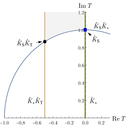
Refer to caption
Figure 3: Fixed points and curves in the moduli space of the Kähler modulus T=Re​T+i​Im​TT=\mathrm{Re}T+\mathrm{i}\,\mathrm{Im}T. The point ⟨T⟩=i\langle T\rangle=\mathrm{i} (blue square) is left fixed by the modular K^S\hat{K}_{\mathrm{S}} transformation, whereas K^S​K^T\hat{K}_{\mathrm{S}}\hat{K}_{\mathrm{T}} leaves ⟨T⟩=ω\langle T\rangle=\omega (black bullet) invariant. These points lie at the intersections of the curves left invariant by the GL⁡(2,ℤ)\mathrm{GL}(2,\mathbbm{Z}) elements indicated next to them. These curves build the boundary of the fundamental domain (shaded region) of the moduli space in the 𝕋2/ℤ3\mathbbm{T}^{2}/\mathbbm{Z}_{3} orbifold sector. We omit the K^S2\hat{K}_{\mathrm{S}}^{2} modular symmetry, which acts trivially on the whole moduli space and is included in the traditional flavor group.

Let us now spend a few words on the case of the 𝕋2/ℤ2\mathbbm{T}^{2}/\mathbbm{Z}_{2} orbifold sector. As detailed in ref. [19], in this case both TT and UU moduli are not fixed. However, one can choose special vevs (⟨T⟩,⟨U⟩)(\langle T\rangle,\langle U\rangle) that are left invariant by a modular stabilizer subgroup H(⟨T⟩,⟨U⟩)H_{(\langle T\rangle,\langle U\rangle)}, which, in contrast to H⟨T⟩H_{\langle T\rangle} in eq. (154), includes elements not only from SL​(2,ℤ)T\mathrm{SL}(2,\mathbbm{Z})_{T}, but from the whole modular group of the orbifold. Hence, the unified flavor symmetry in this case can be expressed analogously to eq. (160), replacing H⟨T⟩H_{\langle T\rangle} by H(⟨T⟩,⟨U⟩)H_{(\langle T\rangle,\langle U\rangle)}.

In the following, we illustrate the scheme of local flavor unification by assuming that the Kähler modulus is stabilized at various different points in moduli space of the 𝕋2/ℤ3\mathbbm{T}^{2}/\mathbbm{Z}_{3} orbifold sector. This moduli space is illustrated in figure 3. We explore first the resulting unified flavor symmetries at the boundaries of the moduli space, depicted by the curves in the figure, where we realize that a unique purely 𝒞​𝒫\mathcal{CP} enhancement of the flavor symmetry occurs. Then, we focus on two self-dual points ⟨T⟩=i\langle T\rangle=\mathrm{i} and ⟨T⟩=ω\langle T\rangle=\omega, displayed in the figure 3 as a (blue) square and a (black) bullet, respectively. Since we suppose the 𝕋2/ℤ3\mathbbm{T}^{2}/\mathbbm{Z}_{3} orbifold sector to be embedded in a six-dimensional orbifold, our starting point is the traditional flavor symmetry Δ′​(54,2,1)≅[162,44]≅Δ⁡(54)∪ℤ9R\Delta^{\prime}(54,2,1)\cong[162,44]\cong\Delta(54)\cup\mathbbm{Z}_{9}^{R}, cf. table 5. Depending on the value of ⟨T⟩\langle T\rangle in moduli space, different unbroken modular transformations contribute to enhance this traditional flavor group to various unified flavor symmetries contained in the full eclectic flavor group, Ω⁡(2)∪ℤ2𝒞​𝒫\Omega(2)\cup\mathbbm{Z}_{2}^{\mathcal{CP}}, which is of order 3,888. A brief summary of these findings is shown in table 6. Furthermore, we study the details of the twisted matter fields Φ−2/3i=(Xi,Yi,Zi)T\Phi_{\nicefrac{{-2}}{{3}}}^{i}=(X_{i},Y_{i},Z_{i})^{\mathrm{T}} and their superpotential eq. (131) compatible with the unbroken symmetries at the different points in moduli space.

6.1 Flavor enhancement at the boundary of the moduli space of 𝕋𝟐/ℤ𝟑\mathbbm{T}^{2}/\mathbbm{Z}_{3}

⟨T⟩\langle T\rangle stabilizer generators unified flavor symmetries
non 𝒞​𝒫\mathcal{CP}-like 𝒞​𝒫\mathcal{CP}-like without 𝒞​𝒫\mathcal{CP} with 𝒞​𝒫\mathcal{CP}
i\mathrm{i} K^S\hat{K}_{\mathrm{S}} K^∗\hat{K}_{*} Ξ⁡(2,2)≅[324,111]\Xi(2,2)\cong[324,111] [648,548][648,548]
ω\omega K^S​K^T\hat{K}_{\mathrm{S}}\hat{K}_{\mathrm{T}} K^∗​K^T\hat{K}_{*}\hat{K}_{\mathrm{T}} H⁡(3,2,1)≅[486,125]H(3,2,1)\cong[486,125] [972,469][972,469]
Re⁡⟨T⟩=0\re\langle T\rangle=0 K^∗\hat{K}_{*} Δ′​(54,2,1)≅[162,44]\Delta^{\prime}(54,2,1)\cong[162,44] [324,125][324,125]
Re⁡⟨T⟩=−1/2\re\langle T\rangle=\nicefrac{{-1}}{{2}} K^∗​K^T\hat{K}_{*}\hat{K}_{\mathrm{T}} Δ′​(54,2,1)≅[162,44]\Delta^{\prime}(54,2,1)\cong[162,44] [324,125][324,125]
|⟨T⟩|=1|\langle T\rangle|=1 K^S​K^∗\hat{K}_{\mathrm{S}}\hat{K}_{*} Δ′​(54,2,1)≅[162,44]\Delta^{\prime}(54,2,1)\cong[162,44] [324,125][324,125]
Table 6: Unified flavor symmetries at different Kähler modulus vevs ⟨T⟩\langle T\rangle of the 𝕋2/ℤ3\mathbbm{T}^{2}/\mathbbm{Z}_{3} orbifold sector embedded in a six-dimensional orbifold. The GL​(2,ℤ)T\mathrm{GL}(2,\mathbbm{Z})_{T} modular transformations that leave ⟨T⟩\langle T\rangle invariant (generating the so-called stabilizer modular subgroup) enhance the traditional flavor symmetry Δ′​(54,2,1)≅Δ⁡(54)∪ℤ9R\Delta^{\prime}(54,2,1)\cong\Delta(54)\cup\mathbbm{Z}_{9}^{R} of the orbifold sector to various large unified flavor symmetries, which generically include 𝒞​𝒫\mathcal{CP}-like transformations. Note that the unified flavor symmetry is unique at all curves depicted in figure 3 that build the boundary of the fundamental domain of the moduli space of TT. Furthermore, since (K^S)2(\hat{K}_{\mathrm{S}})^{2} already belongs to the traditional flavor symmetry, we do not list it here.

Let us begin the discussion of local flavor unification in the 𝕋2/ℤ3\mathbbm{T}^{2}/\mathbbm{Z}_{3} orbifold sector by studying the flavor symmetry enhancement at the various curves in figure 3, which describe the boundary of the fundamental domain in moduli space for the Kähler modulus TT. The three curves are defined by the constraints Re⁡⟨T⟩=0\re\langle T\rangle=0, Re⁡⟨T⟩=−1/2\re\langle T\rangle=\nicefrac{{-1}}{{2}} and |⟨T⟩|=1|\langle T\rangle|=1, respectively. We find that the stabilizer elements H⟨T⟩⊂GL​(2,ℤ)TH_{\langle T\rangle}\subset\mathrm{GL}(2,\mathbbm{Z})_{T} compatible with the previous conditions are generated in each case by

at Re⟨T⟩=0:\displaystyle\text{at }\re\langle T\rangle=0\hskip 14.22636pt: ⟨T⟩→K^∗−⟨T⟩¯=⟨T⟩,\displaystyle\langle T\rangle~\xrightarrow{\hat{K}_{*}}-\bar{\langle T\rangle}~=~\langle T\rangle\,, (161a)
at ​Re⁡⟨T⟩=−1/2:\displaystyle\text{at }\re\langle T\rangle=\nicefrac{{-1}}{{2}}\,: ⟨T⟩→K^∗−⟨T⟩¯→K^T−⟨T⟩¯−1=⟨T⟩,\displaystyle\langle T\rangle~\xrightarrow{\hat{K}_{*}}~-\bar{\langle T\rangle}~\xrightarrow{\hat{K}_{\mathrm{T}}}~-\bar{\langle T\rangle}-1~=~\langle T\rangle\,, (161b)
at |⟨T⟩|=1:\displaystyle\text{at }|\langle T\rangle|=1\hskip 22.76219pt: ⟨T⟩→K^S−1⟨T⟩→K^∗1⟨T⟩¯=⟨T⟩.\displaystyle\langle T\rangle~\xrightarrow{\hat{K}_{\mathrm{S}}}~-\frac{1}{\langle T\rangle}~\xrightarrow{\hat{K}_{*}}~\frac{1}{\bar{\langle T\rangle}}~=~\langle T\rangle\,. (161c)

Besides, we find the unbroken symmetry K^S2\hat{K}_{\mathrm{S}}^{2} that leaves the whole moduli space invariant and satisfies K^S2=C\hat{K}_{\mathrm{S}}^{2}=\mathrm{C}, becoming a symmetry generator already included in the traditional flavor group. Therefore, we find that the stabilizer subgroup is H⟨T⟩=ℤ2×ℤ2𝒞​𝒫H_{\langle T\rangle}=\mathbbm{Z}_{2}\times\mathbbm{Z}_{2}^{\mathcal{CP}}. Note that the stabilizer elements that can enhance the traditional flavor group include the 𝒞​𝒫\mathcal{CP}-like generator K^∗\hat{K}_{*} in all cases. Hence, there is no flavor enhancement without 𝒞​𝒫\mathcal{CP}-like transformations at a generic point on the boundary of the fundamental domain in TT moduli space. That is, ignoring the possibility of 𝒞​𝒫\mathcal{CP}, the traditional flavor symmetry Δ′​(54,2,1)≅Δ⁡(54)∪ℤ9R\Delta^{\prime}(54,2,1)\cong\Delta(54)\cup\mathbbm{Z}_{9}^{R} is not enhanced at the boundaries of the fundamental domain.

In order to figure out the flavor enhancements that the 𝒞​𝒫\mathcal{CP}-like stabilizer elements in eq. (161) induce, we must consider i) the matrix representations of these stabilizer elements when acting on the twisted matter fields Φ−2/3\Phi_{\nicefrac{{-2}}{{3}}} (and their 𝒞​𝒫\mathcal{CP}-conjugate Φ¯−2/3\bar{\Phi}_{\nicefrac{{-2}}{{3}}}), and ii) the automorphy factors associated with these transformations. The representations are obtained as products of ρ⁡(K^S)\rho(\hat{K}_{\mathrm{S}}) and ρ⁡(K^T)\rho(\hat{K}_{\mathrm{T}}) given in eq. (123), as well as ρ⁡(K^∗)\rho(\hat{K}_{*}) defined in eq. (148). Further, by using the 2×22\times 2 matrices that represent the GL​(2,ℤ)T\mathrm{GL}(2,\mathbbm{Z})_{T} generators K^S\hat{K}_{\mathrm{S}}, K^T\hat{K}_{\mathrm{T}} (see eq. (2)) and K^∗\hat{K}_{*} (see eq. (145)), we find that the automorphy factors are trivial for Re⁡⟨T⟩=0,−1/2\re\langle T\rangle=0,\nicefrac{{-1}}{{2}}, i.e.

Φ−2/3\displaystyle\Phi_{\nicefrac{{-2}}{{3}}} →K^∗\displaystyle\xrightarrow{\hat{K}_{*}} Φ¯−2/3,\displaystyle\bar{\Phi}_{\nicefrac{{-2}}{{3}}}\;, (162a)
Φ−2/3\displaystyle\Phi_{\nicefrac{{-2}}{{3}}} →K^∗​K^T\displaystyle\xrightarrow{\hat{K}_{*}\hat{K}_{\mathrm{T}}} ρ​(K^T)∗​Φ¯−2/3.\displaystyle\rho(\hat{K}_{\mathrm{T}})^{*}\,\bar{\Phi}_{\nicefrac{{-2}}{{3}}}\;. (162b)

At the points ⟨T⟩\langle T\rangle satisfying |⟨T⟩|=1|\langle T\rangle|=1, we have

Φ−2/3→K^S​K^∗Φ¯−2/3′=(⟨T¯⟩)−2/3​ρ​(K^S)​Φ¯−2/3.\Phi_{\nicefrac{{-2}}{{3}}}~\xrightarrow{\hat{K}_{\mathrm{S}}\hat{K}_{*}}~\bar{\Phi}^{\prime}_{\nicefrac{{-2}}{{3}}}~=~(\langle\bar{T}\rangle)^{\nicefrac{{-2}}{{3}}}\rho(\hat{K}_{\mathrm{S}})\,\bar{\Phi}_{\nicefrac{{-2}}{{3}}}\,. (163)

In all three cases, one can show easily that H⟨T⟩=ℤ2𝒞​𝒫H_{\langle T\rangle}=\mathbbm{Z}_{2}^{\mathcal{CP}} acts on the matter fields as a ℤ2\mathbbm{Z}_{2} symmetry.33 3 To verify this, one must use ρ⁡(K^T)​ρ​(K^T)∗=ρ⁡(K^S)​ρ​(K^S)∗=𝟙\rho(\hat{K}_{\mathrm{T}})\rho(\hat{K}_{\mathrm{T}})^{*}=\rho(\hat{K}_{\mathrm{S}})\rho(\hat{K}_{\mathrm{S}})^{*}=\mathbbm{1}. Thus, the order of the traditional flavor symmetry is enhanced by a factor of two, resulting in the unified flavor symmetry

Guf,⟨T⟩∈boundary≅Δ′​(54,2,1)∪ℤ2𝒞​𝒫≅[324,125]G_{\mathrm{uf},\langle T\rangle\in\mathrm{boundary}}~\cong~\Delta^{\prime}(54,2,1)\cup\mathbbm{Z}_{2}^{\mathcal{CP}}~\cong~[324,125] (164)

at a generic point on the boundary of the fundamental domain of the TT moduli space.

6.2 Flavor symmetry at ⟨𝑻⟩=𝐢\langle T\rangle=\mathrm{i} in moduli space of 𝕋𝟐/ℤ𝟑\mathbbm{T}^{2}/\mathbbm{Z}_{3}

As one can infer from figure 3, at ⟨T⟩=i\langle T\rangle=\mathrm{i} the stabilizer subgroup includes the SL​(2,ℤ)T\mathrm{SL}(2,\mathbbm{Z})_{T} transformation K^S\hat{K}_{\mathrm{S}},

⟨T⟩⟶K^S−1⟨T⟩=⟨T⟩at⟨T⟩=i,\langle T\rangle~\stackrel{{\scriptstyle\hat{K}_{\mathrm{S}}}}{{\longrightarrow}}~-\frac{1}{\langle T\rangle}~=~\langle T\rangle\quad\mathrm{at}\quad\langle T\rangle~=~\mathrm{i}\;, (165)

and the 𝒞​𝒫\mathcal{CP}-like generator K^∗\hat{K}_{*} because ⟨T⟩=i\langle T\rangle=\mathrm{i} satisfies eq. (161a). Since K^S4=𝟙\hat{K}_{\mathrm{S}}^{4}=\mathbbm{1}, the full stabilizer subgroup is Hi≅ℤ4×ℤ2𝒞​𝒫H_{\mathrm{i}}\cong\mathbbm{Z}_{4}\times\mathbbm{Z}_{2}^{\mathcal{CP}}, where the ℤ2⊂ℤ4\mathbbm{Z}_{2}\subset\mathbbm{Z}_{4} subgroup associated with K^S2=C\hat{K}_{\mathrm{S}}^{2}=\mathrm{C} (see eq. (130)) already belongs to the traditional flavor symmetry Δ⁡(54)⊂Δ′​(54,2,1)\Delta(54)\subset\Delta^{\prime}(54,2,1).

As the vev ⟨T⟩=i\langle T\rangle=\mathrm{i} of the modulus is invariant under HiH_{\mathrm{i}}, the coupling strengths Y^1​(⟨T⟩)\hat{Y}_{1}(\langle T\rangle) and Y^2​(⟨T⟩)\hat{Y}_{2}(\langle T\rangle) are also invariant. Using the general modular transformations eq. (119), this implies particularly that the K^S\hat{K}_{\mathrm{S}} transformation on the coupling strengths leads to

Y^𝟐′′(1)​(i)=(Y^1​(i)Y^2​(i))⟶K^S(Y^1​(−1i)Y^2​(−1i))=−13​(122−1)​(Y^1​(i)Y^2​(i))=(Y^1​(i)Y^2​(i)).\hat{Y}^{(1)}_{\boldsymbol{2}^{\prime\prime}}(\mathrm{i})~=~\begin{pmatrix}\hat{Y}_{1}(\mathrm{i})\\ \hat{Y}_{2}(\mathrm{i})\end{pmatrix}~\stackrel{{\scriptstyle\hat{K}_{\mathrm{S}}}}{{\longrightarrow}}~\begin{pmatrix}\hat{Y}_{1}\left(-\frac{1}{\mathrm{i}}\right)\\ \hat{Y}_{2}\left(-\frac{1}{\mathrm{i}}\right)\end{pmatrix}~=~-\frac{1}{\sqrt{3}}\,\begin{pmatrix}1&\sqrt{2}\\ \sqrt{2}&-1\end{pmatrix}\begin{pmatrix}\hat{Y}_{1}(\mathrm{i})\\ \hat{Y}_{2}(\mathrm{i})\end{pmatrix}~=~\begin{pmatrix}\hat{Y}_{1}(\mathrm{i})\\ \hat{Y}_{2}(\mathrm{i})\end{pmatrix}\;. (166)

Consequently, the doublet of couplings Y^𝟐′′(1)​(i)\hat{Y}^{(1)}_{\boldsymbol{2}^{\prime\prime}}(\mathrm{i}) is an eigenvector of the matrix ρ𝟐′′​(K^S)\rho_{\boldsymbol{2}^{\prime\prime}}(\hat{K}_{\mathrm{S}}) with eigenvalue i\mathrm{i}. Thus, eq. (166) amounts to the vev alignment

Y^𝟐′′(1)​(i)=Y^2​(i)​(−21+31),\hat{Y}^{(1)}_{\boldsymbol{2}^{\prime\prime}}(\mathrm{i})~=~\hat{Y}_{2}(\mathrm{i})\left(\begin{array}[]{c}-\frac{\sqrt{2}}{1+\sqrt{3}}\\ 1\end{array}\right)\;, (167)

which provides a nontrivial relation between Y^1​(i)\hat{Y}_{1}(\mathrm{i}) and Y^2​(i)\hat{Y}_{2}(\mathrm{i}). As a side remark, because of the vev alignment eq. (167), the T′T^{\prime} modular forms Y^𝟏(4)​(T)\hat{Y}^{(4)}_{\boldsymbol{1}}(T), Y^𝟏′(4)​(T)\hat{Y}^{(4)}_{\boldsymbol{1}^{\prime}}(T) and Y^𝟑(4)​(T)\hat{Y}^{(4)}_{\boldsymbol{3}}(T) of weight 44 given in ref. [3] get aligned at ⟨T⟩=i\langle T\rangle=\mathrm{i} as

Y^𝟏(4)​(i)=Y𝟏′(4)​(i)=3​(3−2​3)​Y^2​(i)4andY^𝟑(4)​(i)=3​(2−3)​Y^2​(i)4​(11−1).\hat{Y}^{(4)}_{\boldsymbol{1}}(\mathrm{i})~=~Y^{(4)}_{\boldsymbol{1}^{\prime}}(\mathrm{i})~=~3(3-2\sqrt{3})\,\hat{Y}_{2}(\mathrm{i})^{4}\quad\mathrm{and}\quad\hat{Y}^{(4)}_{\boldsymbol{3}}(\mathrm{i})~=~3(2-\sqrt{3})\,\hat{Y}_{2}(\mathrm{i})^{4}\left(\begin{array}[]{c}1\\ 1\\ -1\end{array}\right)\;. (168)

Furthermore, both modular forms, Y^1​(i)\hat{Y}_{1}(\mathrm{i}) and Y^2​(i)\hat{Y}_{2}(\mathrm{i}), are real at ⟨T⟩=i\langle T\rangle=\mathrm{i} (as one can also infer directly from eq. (149)) and we find

Y^1​(i)=−3​2​η3​(3​i)η⁡(i)≈−0.5234andY^2​(i)≈1.0112.\hat{Y}_{1}(\mathrm{i})~=~-3\sqrt{2}\frac{\eta^{3}(3\,\mathrm{i})}{\eta(\mathrm{i})}~\approx~-0.5234\quad\mathrm{and}\quad\hat{Y}_{2}(\mathrm{i})~\approx~1.0112\;. (169)

We can apply the vev alignment eq. (167) also to the trilinear superpotential eq. (131) of twisted matter fields Φ−2/3i=(Xi,Yi,Zi)T\Phi_{\nicefrac{{-2}}{{3}}}^{i}=(X_{i},Y_{i},Z_{i})^{\mathrm{T}}, i=1,2,3i=1,2,3. At ⟨T⟩=i\langle T\rangle=\mathrm{i}, it turns out that

𝒲⁡(i,Xi,Yi,Zi)\displaystyle\mathcal{W}(\mathrm{i},X_{i},Y_{i},Z_{i}) ⊃\displaystyle\supset c(1)Y^2(i)[(X1X2X3+Y1Y2Y3+Z1Z2Z3)\displaystyle c^{(1)}\,\hat{Y}_{2}(\mathrm{i})\Big[\big(X_{1}\,X_{2}\,X_{3}+Y_{1}\,Y_{2}\,Y_{3}+Z_{1}\,Z_{2}\,Z_{3}\big) (170b)
+11+3​(X1​Y2​Z3+X1​Y3​Z2+X2​Y1​Z3CLOSE\displaystyle+\frac{1}{1+\sqrt{3}}\big(X_{1}\,Y_{2}\,Z_{3}+X_{1}\,Y_{3}\,Z_{2}+X_{2}\,Y_{1}\,Z_{3}
+X3Y1Z2+X2Y3Z1+X3Y2Z1)].\displaystyle\hskip 44.10185pt+X_{3}\,Y_{1}\,Z_{2}+X_{2}\,Y_{3}\,Z_{1}+X_{3}\,Y_{2}\,Z_{1}\big)\Big]\;.

Under a modular K^S\hat{K}_{\mathrm{S}} transformation with its representation given by eq. (123), twisted matter fields transform, according to eq. (157), as

(XiYiZi)⟶K^S(Xi′Yi′Zi′)=i​(−i)−2/33​(1111ω2ω1ωω2)⏟=:ρ𝟑2,i​(K^S)(XiYiZi),\left(\begin{array}[]{c}X_{i}\\ Y_{i}\\ Z_{i}\end{array}\right)~\stackrel{{\scriptstyle\hat{K}_{\mathrm{S}}}}{{\longrightarrow}}~\left(\begin{array}[]{c}X_{i}^{\prime}\\ Y_{i}^{\prime}\\ Z_{i}^{\prime}\end{array}\right)~=~\underbrace{\frac{\mathrm{i}(-\mathrm{i})^{\nicefrac{{-2}}{{3}}}}{\sqrt{3}}\left(\begin{array}[]{ccc}1&1&1\\ 1&\omega^{2}&\omega\\ 1&\omega&\omega^{2}\end{array}\right)}_{=:~\rho_{\boldsymbol{3}_{2},\mathrm{i}}(\hat{K}_{\mathrm{S}})}\left(\begin{array}[]{c}X_{i}\\ Y_{i}\\ Z_{i}\end{array}\right)\;, (171)

where the multivalued factor (−i)−2/3(-\mathrm{i})^{\nicefrac{{-2}}{{3}}} can be fixed to −ω2=exp⁡(π​i/3)-\omega^{2}=\exp(\nicefrac{{\pi\mathrm{i}}}{{3}}) by the ℤ3\mathbbm{Z}_{3} point group symmetry, and the representation 𝒕=𝟑2\boldsymbol{t}=\boldsymbol{3}_{2} following the notation of eq. (157) corresponds to the triplet that the matter fields build in the resulting unified flavor symmetry at ⟨T⟩=i\langle T\rangle=\mathrm{i}. It then follows that K^S\hat{K}_{\mathrm{S}} acts on the superpotential evaluated at ⟨T⟩=i\langle T\rangle=\mathrm{i} as an RR-symmetry,

𝒲⁡(i,Xi,Yi,Zi)⟶K^S𝒲⁡(i,Xi′,Yi′,Zi′)=i​𝒲​(i,Xi,Yi,Zi),\mathcal{W}(\mathrm{i},X_{i},Y_{i},Z_{i})~\stackrel{{\scriptstyle\hat{K}_{\mathrm{S}}}}{{\longrightarrow}}~\mathcal{W}(\mathrm{i},X_{i}^{\prime},Y_{i}^{\prime},Z_{i}^{\prime})~=~\mathrm{i}\,\mathcal{W}(\mathrm{i},X_{i},Y_{i},Z_{i})\;, (172)

as one can also see directly from eq. (46a). Moreover, due to ρ𝟑2,i​(K^S)\rho_{\boldsymbol{3}_{2},\mathrm{i}}(\hat{K}_{\mathrm{S}}), the modular K^S\hat{K}_{\mathrm{S}} transformation at ⟨T⟩=i\langle T\rangle=\mathrm{i} generates a ℤ12≅ℤ4×ℤ3\mathbbm{Z}_{12}\cong\mathbbm{Z}_{4}\times\mathbbm{Z}_{3} traditional flavor symmetry when acting on matter fields, cf. eq. (171), where ℤ4×ℤ3\mathbbm{Z}_{4}\times\mathbbm{Z}_{3} can be generated by

(ρ𝟑2,i​(K^S))3=i3​(1111ωω21ω2ω)and(ρ𝟑2,i​(K^S))4=ω2​𝟙,\left(\rho_{\boldsymbol{3}_{2},\mathrm{i}}(\hat{K}_{\mathrm{S}})\right)^{3}~=~\frac{\mathrm{i}}{\sqrt{3}}\left(\begin{array}[]{ccc}1&1&1\\ 1&\omega&\omega^{2}\\ 1&\omega^{2}&\omega\end{array}\right)\qquad\mathrm{and}\qquad\left(\rho_{\boldsymbol{3}_{2},\mathrm{i}}(\hat{K}_{\mathrm{S}})\right)^{4}~=~\omega^{2}\mathbbm{1}\;, (173)

respectively. It is easy to see that the ℤ4\mathbbm{Z}_{4} factor generated by (ρ𝟑2,i​(K^S))3(\rho_{\boldsymbol{3}_{2},\mathrm{i}}(\hat{K}_{\mathrm{S}}))^{3} is an RR-symmetry, while the ℤ3\mathbbm{Z}_{3} factor generated by (ρ𝟑2,i​(K^S))4(\rho_{\boldsymbol{3}_{2},\mathrm{i}}(\hat{K}_{\mathrm{S}}))^{4} is equivalent to the point group symmetry (129a) of the orbifold sector.44 4 The transformation K^S3\hat{K}_{\mathrm{S}}^{3} at ⟨T⟩=i\langle T\rangle=\mathrm{i} acts as a ℤ4\mathbbm{Z}_{4} on bosons and on 𝒲\mathcal{W}. However, due to eq. (159), it is actually an ℤ8\mathbbm{Z}_{8} RR-symmetry when acting on fermions. Since discrete RR-symmetries are relevant for phenomenology [61, 62], it may be interesting to explore the consequences of this symmetry. Using that (ρ𝟑2,i​(K^S))6=ρ𝟑2​(C)(\rho_{\boldsymbol{3}_{2},\mathrm{i}}(\hat{K}_{\mathrm{S}}))^{6}=\rho_{\boldsymbol{3}_{2}}\!(\mathrm{C}), without including 𝒞​𝒫\mathcal{CP}-like transformations the traditional flavor symmetry is enhanced from

Δ′​(54,2,1)toΞ⁡(2,2)≅[324,111]at ​⟨T⟩=i.\Delta^{\prime}(54,2,1)\qquad\text{to}\qquad\Xi(2,2)~\cong~[324,111]\qquad\text{at }\langle T\rangle=\mathrm{i}\;. (174)

This is the largest traditional flavor group without 𝒞​𝒫\mathcal{CP} that can be obtained in the 𝕋2/ℤ3\mathbbm{T}^{2}/\mathbbm{Z}_{3} orbifold sector embedded in a higher-dimensional orbifold, and contains the group Σ⁡(36×3)≅[108,15]\Sigma(36\times 3)\cong[108,15] that results when the discrete ℤ9R\mathbbm{Z}_{9}^{R} RR-symmetry from SL​(2,ℤ)U\mathrm{SL}(2,\mathbbm{Z})_{U} is not considered [17, 18, 3]. Similarly to that case, the Ξ⁡(2,2)\Xi(2,2) group can be generated by the matrices ρ⁡(A)\rho(\mathrm{A}), ρ⁡(B)\rho(\mathrm{B}) given in eq. (127), the ℤ9R\mathbbm{Z}_{9}^{R} generator ρ⁡(R^1)\rho(\hat{\mathrm{R}}_{1}) eq. (139), and ρ𝟑2,i​(K^S)\rho_{\boldsymbol{3}_{2},\mathrm{i}}(\hat{K}_{\mathrm{S}}) in the faithful triplet representation 𝟑2\boldsymbol{3}_{2} of Ξ⁡(2,2)\Xi(2,2).

As a side remark, the relation ρ𝟑2,i​(K^S4)=(ρ𝟑2,i​(K^S))4=ω2​𝟙\rho_{\boldsymbol{3}_{2},\mathrm{i}}(\hat{K}_{\mathrm{S}}^{4})=(\rho_{\boldsymbol{3}_{2},\mathrm{i}}(\hat{K}_{\mathrm{S}}))^{4}=\omega^{2}\mathbbm{1} in eq. (173) is a consistent representation of K^S4=𝟙\hat{K}_{\mathrm{S}}^{4}=\mathbbm{1} (see eq. (1)) because the latter indicates that K^S4\hat{K}_{\mathrm{S}}^{4} must act trivially on the fields up to the action of the traditional flavor symmetry.

So far, we have not yet considered the ℤ2𝒞​𝒫\mathbbm{Z}_{2}^{\mathcal{CP}} 𝒞​𝒫\mathcal{CP}-like transformation K^∗\hat{K}_{*} at ⟨T⟩=i\langle T\rangle=\mathrm{i}. Using the 𝒞​𝒫\mathcal{CP}-like transformation (162a) of matter fields, one can explicitly show that

𝒲⁡(i,Xi,Yi,Zi)⟶K^∗𝒲⁡(i,X¯i,Y¯i,Z¯i)=(𝒲⁡(i,Xi,Yi,Zi))∗,\mathcal{W}(\mathrm{i},X_{i},Y_{i},Z_{i})~\stackrel{{\scriptstyle\hat{K}_{*}}}{{\longrightarrow}}~\mathcal{W}(\mathrm{i},\bar{X}_{i},\bar{Y}_{i},\bar{Z}_{i})~=~\big(\mathcal{W}(\mathrm{i},X_{i},Y_{i},Z_{i})\big)^{*}\;, (175)

using the superpotential eq. (170) with c(1)​Y^2​(i)∈ℝc^{(1)}\,\hat{Y}_{2}(\mathrm{i})\in\mathbbm{R} and the discussion on 𝒞​𝒫\mathcal{CP} from section 5.7. Consequently, if we stabilize the Kähler modulus TT at ⟨T⟩=i\langle T\rangle=\mathrm{i}, the trilinear superpotential eq. (170) respects 𝒞​𝒫\mathcal{CP}. Including 𝒞​𝒫\mathcal{CP}, the unified flavor group at ⟨T⟩=i\langle T\rangle=\mathrm{i} is given by

Guf,⟨T⟩=i≅[648,548]≅Δ′​(54,2,1)∪ℤ4∪ℤ2𝒞​𝒫,G_{\mathrm{uf},\langle T\rangle=\mathrm{i}}~\cong~[648,548]~\cong~\Delta^{\prime}(54,2,1)\cup\mathbbm{Z}_{4}\cup\mathbbm{Z}_{2}^{\mathcal{CP}}\;, (176)

where Ξ⁡(2,2)≅Δ′​(54,2,1)∪ℤ4\Xi(2,2)\cong\Delta^{\prime}(54,2,1)\cup\mathbbm{Z}_{4} is the maximal flavor subgroup of Guf,⟨T⟩=iG_{\mathrm{uf},\langle T\rangle=\mathrm{i}} which does not act 𝒞​𝒫\mathcal{CP}-like.

6.3 Flavor symmetry at ⟨𝑻⟩=𝝎\langle T\rangle=\omega in moduli space of 𝕋𝟐/ℤ𝟑\mathbbm{T}^{2}/\mathbbm{Z}_{3}

Let us now assume that the Kähler modulus is stabilized at ⟨T⟩=ω\langle T\rangle=\omega in moduli space. There, as illustrated in figure 3, the unbroken GL​(2,ℤ)T\mathrm{GL}(2,\mathbbm{Z})_{T} symmetries can be generated by the ℤ2𝒞​𝒫\mathbbm{Z}_{2}^{\mathcal{CP}} 𝒞​𝒫\mathcal{CP}-like transformation K^∗​K^T\hat{K}_{*}\hat{K}_{\mathrm{T}}, and the ℤ3\mathbbm{Z}_{3} modular transformation K^S​K^T\hat{K}_{\mathrm{S}}\hat{K}_{\mathrm{T}},

⟨T⟩⟶K^S−1⟨T⟩⟶K^T−1⟨T⟩+1=⟨T⟩.\langle T\rangle~\stackrel{{\scriptstyle\hat{K}_{\mathrm{S}}}}{{\longrightarrow}}~-\frac{1}{\langle T\rangle}~\stackrel{{\scriptstyle\hat{K}_{\mathrm{T}}}}{{\longrightarrow}}~-\frac{1}{\langle T\rangle+1}~=~\langle T\rangle\;. (177)

In addition, we have the ℤ2\mathbbm{Z}_{2} transformation K^S2=C\hat{K}_{\mathrm{S}}^{2}=\mathrm{C} that is already included in the traditional flavor group. The resulting stabilizer subgroup reads Hω≅ℤ3×ℤ2×ℤ2𝒞​𝒫H_{\omega}\cong\mathbbm{Z}_{3}\times\mathbbm{Z}_{2}\times\mathbbm{Z}_{2}^{\mathcal{CP}}.

At this point in moduli space, the coupling strengths governed by the modular forms Y^1​(⟨T⟩)\hat{Y}_{1}(\langle T\rangle) and Y^2​(⟨T⟩)\hat{Y}_{2}(\langle T\rangle) with modular weight nY=1n_{Y}=1 get aligned as

Y^𝟐′′(1)​(ω)=Y^2​(ω)​(12​ω1),whereY^2​(ω)≈0.97399899.\hat{Y}^{(1)}_{\boldsymbol{2}^{\prime\prime}}(\omega)~=~\hat{Y}_{2}(\omega)\left(\begin{array}[]{c}\frac{1}{\sqrt{2}}\omega\\ 1\end{array}\right)\,,\quad\mathrm{where}\quad\hat{Y}_{2}(\omega)~\approx~0.97399899\;. (178)

Incidentally, the vev alignment given by eq. (178) implies that the T′T^{\prime} modular forms Y^𝟏(4)​(T)\hat{Y}^{(4)}_{\boldsymbol{1}}(T), Y^𝟏′(4)​(T)\hat{Y}^{(4)}_{\boldsymbol{1}^{\prime}}(T) and Y^𝟑(4)​(T)\hat{Y}^{(4)}_{\boldsymbol{3}}(T) of weight 44 given in ref. [3] are aligned at ⟨T⟩=ω\langle T\rangle=\omega according to

Y^𝟏(4)​(ω)=0,Y^𝟏′(4)​(ω)=94​ω​Y^2​(ω)4andY^𝟑(4)​(ω)=32​Y^2​(ω)4​(1−12​ω−ω2).\hat{Y}^{(4)}_{\boldsymbol{1}}(\omega)~=~0\quad,\quad\hat{Y}^{(4)}_{\boldsymbol{1}^{\prime}}(\omega)~=~\frac{9}{4}\omega\hat{Y}_{2}(\omega)^{4}\quad\mathrm{and}\quad\hat{Y}^{(4)}_{\boldsymbol{3}}(\omega)~=~\frac{3}{2}\,\hat{Y}_{2}(\omega)^{4}\left(\begin{array}[]{c}1\\ -\frac{1}{2}\omega\\ -\omega^{2}\end{array}\right)\;. (179)

On the other hand, in this case the trilinear superpotential eq. (131) simplifies to

𝒲⁡(ω,Xi,Yi,Zi)\displaystyle\mathcal{W}(\omega,X_{i},Y_{i},Z_{i}) ⊃\displaystyle\supset c(1)Y^2(ω)[X1X2X3+Y1Y2Y3+Z1Z2Z3\displaystyle c^{(1)}\,\hat{Y}_{2}(\omega)\Big[X_{1}\,X_{2}\,X_{3}+Y_{1}\,Y_{2}\,Y_{3}+Z_{1}\,Z_{2}\,Z_{3} (180a)
−ω2​(X1​Y2​Z3+X1​Y3​Z2+X2​Y1​Z3CLOSE\displaystyle\hskip 45.5244pt-\frac{\omega}{2}\big(X_{1}\,Y_{2}\,Z_{3}+X_{1}\,Y_{3}\,Z_{2}+X_{2}\,Y_{1}\,Z_{3} (180b)
+X3Y1Z2+X2Y3Z1+X3Y2Z1)].\displaystyle\hskip 56.9055pt+\,X_{3}\,Y_{1}\,Z_{2}+X_{2}\,Y_{3}\,Z_{1}+X_{3}\,Y_{2}\,Z_{1}\big)\Big]\;.

Under a modular K^S​K^T\hat{K}_{\mathrm{S}}\,\hat{K}_{\mathrm{T}} transformation at ⟨T⟩=ω\langle T\rangle=\omega, the three triplets of twisted matter fields Φ−2/3i\Phi_{\nicefrac{{-2}}{{3}}}^{i} transform as

(XiYiZi)→K^S​K^T(Xi′Yi′Zi′)=i​(ω2)−2/33​(ω211ω2ω2ωω2ωω2)⏟=:ρ𝟑2,ω​(K^S​K^T)(XiYiZi),\left(\begin{array}[]{c}X_{i}\\ Y_{i}\\ Z_{i}\end{array}\right)~\xrightarrow{\hat{K}_{\mathrm{S}}\,\hat{K}_{\mathrm{T}}}~\left(\begin{array}[]{c}X_{i}^{\prime}\\ Y_{i}^{\prime}\\ Z_{i}^{\prime}\end{array}\right)=\underbrace{\frac{\mathrm{i}\left(\omega^{2}\right)^{\nicefrac{{-2}}{{3}}}}{\sqrt{3}}\left(\begin{array}[]{ccc}\omega^{2}&1&1\\ \omega^{2}&\omega^{2}&\omega\\ \omega^{2}&\omega&\omega^{2}\end{array}\right)}_{=:~\rho_{\boldsymbol{3}_{2},\omega}(\hat{K}_{\mathrm{S}}\,\hat{K}_{\mathrm{T}})}\left(\begin{array}[]{c}X_{i}\\ Y_{i}\\ Z_{i}\end{array}\right)\;, (181)

where 𝒕=𝟑2\boldsymbol{t}=\boldsymbol{3}_{2} denotes the triplet representation of the twisted matter fields Φ−2/3i\Phi_{\nicefrac{{-2}}{{3}}}^{i} under the unified flavor symmetry at ⟨T⟩=ω\langle T\rangle=\omega. We used eq. (123) for ρ⁡(K^S)\rho(\hat{K}_{\mathrm{S}}) and ρ⁡(K^T)\rho(\hat{K}_{\mathrm{T}}), and the automorphy factor (−⟨T⟩−1)−2/3=(ω2)−2/3(-\langle T\rangle-1)^{\nicefrac{{-2}}{{3}}}=(\omega^{2})^{\nicefrac{{-2}}{{3}}} for γT=K^S​K^T\gamma_{T}=\hat{K}_{\mathrm{S}}\,\hat{K}_{\mathrm{T}} evaluated at ⟨T⟩=ω\langle T\rangle=\omega in moduli space, see eq. (157). Note that the multivalued factor (ω2)−2/3\left(\omega^{2}\right)^{\nicefrac{{-2}}{{3}}} can be fixed to exp⁡(2​π​i​ 2/9)\exp(\nicefrac{{2\pi\mathrm{i}\,2}}{{9}}) by the ℤ3(P​G)\mathbbm{Z}_{3}^{(PG)} point group symmetry of the 𝕋2/ℤ3\mathbbm{T}^{2}/\mathbbm{Z}_{3} orbifold sector, see eq. (129a). Due to this phase, ρ𝟑2,ω​(K^S​K^T)\rho_{\boldsymbol{3}_{2},\omega}(\hat{K}_{\mathrm{S}}\,\hat{K}_{\mathrm{T}}) generates a ℤ9\mathbbm{Z}_{9} symmetry that contains the ℤ3(P​G)\mathbbm{Z}_{3}^{(PG)} point group symmetry as a subgroup,

(ρ𝟑2,ω​(K^S​K^T))3=ω2​𝟙.(\rho_{\boldsymbol{3}_{2},\omega}(\hat{K}_{\mathrm{S}}\,\hat{K}_{\mathrm{T}}))^{3}~=~\omega^{2}\mathbbm{1}\;. (182)

Thus, even though ρ𝟑2,ω​(K^S​K^T)\rho_{\boldsymbol{3}_{2},\omega}(\hat{K}_{\mathrm{S}}\,\hat{K}_{\mathrm{T}}) has order 9, the traditional flavor symmetry (without 𝒞​𝒫\mathcal{CP}) is only enhanced from

Δ′​(54,2,1)≅[162,44]toH⁡(3,2,1)≅[486,125]at ​⟨T⟩=ω,\Delta^{\prime}(54,2,1)\cong[162,44]\qquad\mathrm{to}\qquad H(3,2,1)\cong[486,125]\qquad\text{at }\langle T\rangle=\omega\;, (183)

i.e. the order increases by a factor of three (see ref. [51] for the nomenclature).

It follows that the ℤ9⊂H⁡(3,2,1)\mathbbm{Z}_{9}\subset H(3,2,1) transformation eq. (181) acts on the superpotential eq. (180) as

𝒲⁡(ω,Xi,Yi,Zi)→K^S​K^T𝒲⁡(ω,Xi′,Yi′,Zi′)=ω​𝒲​(ω,Xi,Yi,Zi).\mathcal{W}(\omega,X_{i},Y_{i},Z_{i})~\xrightarrow{\hat{K}_{\mathrm{S}}\,\hat{K}_{\mathrm{T}}}~\mathcal{W}(\omega,X_{i}^{\prime},Y_{i}^{\prime},Z_{i}^{\prime})~=~\omega\,\mathcal{W}(\omega,X_{i},Y_{i},Z_{i})\;. (184)

This is expected due to the automorphy factor (−⟨T⟩−1)−1=ω(-\langle T\rangle-1)^{-1}=\omega of the superpotential 𝒲\mathcal{W} for γT=K^S​K^T\gamma_{T}=\hat{K}_{\mathrm{S}}\,\hat{K}_{\mathrm{T}} evaluated at the point ⟨T⟩=ω\langle T\rangle=\omega in moduli space. Thus, the ℤ9\mathbbm{Z}_{9} symmetry enhancement yields a discrete RR-symmetry.

Let us now consider also the 𝒞​𝒫\mathcal{CP}-like transformation K^∗​K^T\hat{K}_{*}\hat{K}_{\mathrm{T}} included in HωH_{\omega}. Under K^∗​K^T\hat{K}_{*}\hat{K}_{\mathrm{T}}, twisted matter fields Φ−2/3i\Phi_{\nicefrac{{-2}}{{3}}}^{i} transform according to eq. (162b), which in terms of the component fields reads (Xi,Yi,Zi)T→K^∗​K^T(ω​X¯i,Y¯i,Z¯i)T(X_{i},Y_{i},Z_{i})^{\mathrm{T}}\xrightarrow{\hat{K}_{*}\hat{K}_{\mathrm{T}}}(\omega\bar{X}_{i},\bar{Y}_{i},\bar{Z}_{i})^{\mathrm{T}}. Then, we find that the superpotential at ⟨T⟩=ω\langle T\rangle=\omega, eq. (180), respects 𝒞​𝒫\mathcal{CP}-like transformations, i.e.

𝒲⁡(ω,Xi,Yi,Zi)→K^∗​K^T𝒲⁡(ω,ω​X¯i,Y¯i,Z¯i)=(𝒲⁡(ω,Xi,Yi,Zi))∗.\mathcal{W}(\omega,X_{i},Y_{i},Z_{i})~\xrightarrow{\hat{K}_{*}\hat{K}_{\mathrm{T}}}~\mathcal{W}(\omega,\omega\bar{X}_{i},\bar{Y}_{i},\bar{Z}_{i})~=~\big(\mathcal{W}(\omega,X_{i},Y_{i},Z_{i})\big)^{*}\;. (185)

This can be easily confirmed by applying the identities

Y^1​(ω)​ω=(Y^1​(ω))∗andY^2​(ω)=(Y^2​(ω))∗,\hat{Y}_{1}(\omega)\omega~=~\left(\hat{Y}_{1}(\omega)\right)^{*}\quad\mathrm{and}\quad\hat{Y}_{2}(\omega)~=~\left(\hat{Y}_{2}(\omega)\right)^{*}\;, (186)

which follow from eqs. (119) and (149). Finally, we find that this 𝒞​𝒫\mathcal{CP} enhancement leads to the unified flavor symmetry given by

Guf,⟨T⟩=ω≅[972,469]≅Δ′​(54,2,1)∪ℤ9∪ℤ2𝒞​𝒫,G_{\mathrm{uf},\langle T\rangle=\omega}~\cong~[972,469]~\cong~\Delta^{\prime}(54,2,1)\cup\mathbbm{Z}_{9}\cup\mathbbm{Z}_{2}^{\mathcal{CP}}\;, (187)

where H⁡(3,2,1)≅Δ′​(54,2,1)∪ℤ9H(3,2,1)\cong\Delta^{\prime}(54,2,1)\cup\mathbbm{Z}_{9} is the maximal flavor subgroup of Guf,⟨T⟩=ωG_{\mathrm{uf},\langle T\rangle=\omega} which does not act 𝒞​𝒫\mathcal{CP}-like.

6.4 Gauge symmetry enhancement at ⟨𝑻⟩=𝝎\langle T\rangle=\omega

Let us analyze the “accidental” continuous symmetries of the superpotential eq. (180) at ⟨T⟩=ω\langle T\rangle=\omega in moduli space. We assume that the twisted matter fields Φ−2/3i=(Xi,Yi,Zi)T\Phi_{\nicefrac{{-2}}{{3}}}^{i}=(X_{i},Y_{i},Z_{i})^{\mathrm{T}} transform identically for i∈{1,2,3}i\in\{1,2,3\} (typically the three copies of twisted matter fields Φ−2/3i\Phi_{\nicefrac{{-2}}{{3}}}^{i} differ in some other gauge charges, such that there is no flavor symmetry that mixes i∈{1,2,3}i\in\{1,2,3\}). To identify continuous symmetries, we define a general infinitesimal U⁡(3)\mathrm{U}(3) transformation

(XiYiZi)⟶U⁡(3)(𝟙3+i​αa​Ta)​(XiYiZi),\begin{pmatrix}X_{i}\\ Y_{i}\\ Z_{i}\end{pmatrix}~\stackrel{{\scriptstyle\mathrm{U}(3)}}{{\longrightarrow}}~\left(\mathbbm{1}_{3}+\mathrm{i}\,\alpha_{a}\,\mathrm{T}_{a}\right)\,\begin{pmatrix}X_{i}\\ Y_{i}\\ Z_{i}\end{pmatrix}\;, (188)

where summation over a=1,…,9a=1,\ldots,9 is implied and the 3×33\times 3 matrices Ta\mathrm{T}_{a} denote the Hermitian generators of the U⁡(3)\mathrm{U}(3) Lie algebra. By demanding invariance of the superpotential eq. (180) at leading order in the parameters αa\alpha_{a}, we obtain two linear independent generators ta\mathrm{t}_{a} that we choose as

t1:=13​2​(0ω2ω2ω01ω10)andt2:=i3​2​(0ω2−ω2−ω01ω−10).\mathrm{t}_{1}~:=~\frac{1}{3\sqrt{2}}\begin{pmatrix}0&\omega^{2}&\omega^{2}\\ \omega&0&1\\ \omega&1&0\end{pmatrix}\quad\mathrm{and}\quad\mathrm{t}_{2}~:=~\frac{\mathrm{i}}{3\sqrt{2}}\begin{pmatrix}0&\omega^{2}&-\omega^{2}\\ -\omega&0&1\\ \omega&-1&0\end{pmatrix}\;. (189)

Note that t1​t2=t2​t1\mathrm{t}_{1}\,\mathrm{t}_{2}=\mathrm{t}_{2}\,\mathrm{t}_{1}. Hence, we found a U⁡(1)×U⁡(1)\mathrm{U}(1)\times\mathrm{U}(1) symmetry of the superpotential eq. (180) at ⟨T⟩=ω\langle T\rangle=\omega. In a full string discussion (see e.g. [41]), one can show that this “accidental” symmetry is actually an exact gauge symmetry, where the U⁡(1)\mathrm{U}(1) gauge bosons correspond to certain winding strings that become massless at the self-dual point ⟨T⟩=ω\langle T\rangle=\omega in moduli space.

Next, we diagonalize the U⁡(1)\mathrm{U}(1) generators eq. (189) simultaneously by performing a (unitary) basis change in field space, i.e.

(XigYigZig):=Mg​(XiYiZi)whereMg:=13​(1ω2ω211ω1ω1),\begin{pmatrix}X^{\mathrm{g}}_{i}\\ Y^{\mathrm{g}}_{i}\\ Z^{\mathrm{g}}_{i}\end{pmatrix}~:=~M^{\mathrm{g}}\,\begin{pmatrix}X_{i}\\ Y_{i}\\ Z_{i}\end{pmatrix}\quad\mathrm{where}\quad M^{\mathrm{g}}~:=~\frac{1}{\sqrt{3}}\begin{pmatrix}1&\omega^{2}&\omega^{2}\\ 1&1&\omega\\ 1&\omega&1\end{pmatrix}\;, (190)

where the superscript character “g” labels the “gauge” basis, in which the U⁡(1)\mathrm{U}(1) generators are diagonal. In this basis, the U⁡(1)\mathrm{U}(1) generators tag:=Mg​ta​(Mg)−1\mathrm{t}^{\mathrm{g}}_{a}:=M^{\mathrm{g}}\,\mathrm{t}_{a}\,(M^{\mathrm{g}})^{-1} for a∈{1,2}a\in\{1,2\} read

t1g=13​2​(2000−1000−1)andt2g=16​(00001000−1).\mathrm{t}^{\mathrm{g}}_{1}~=~\frac{1}{3\sqrt{2}}\begin{pmatrix}2&0&0\\ 0&-1&0\\ 0&0&-1\end{pmatrix}\quad\mathrm{and}\quad\mathrm{t}^{\mathrm{g}}_{2}~=~\frac{1}{\sqrt{6}}\begin{pmatrix}0&0&0\\ 0&1&0\\ 0&0&-1\end{pmatrix}\;. (191)

This reproduces the U⁡(1)\mathrm{U}(1) charges of ℤ3\mathbbm{Z}_{3} twisted strings (M1,M2,M3)(M_{1},M_{2},M_{3}) computed using a ℤ3\mathbbm{Z}_{3} shift orbifold, see ref. [41] and especially table 2 therein. Next, we change the basis for the generators ρ⁡(A)\rho(\mathrm{A}), ρ⁡(B)\rho(\mathrm{B}) and ρ⁡(C)\rho(\mathrm{C}) of the traditional flavor group Δ⁡(54)\Delta(54) given in eqs. (127) and (130). We obtain

ρg(A):=(00ω2ω00010),ρg(B):=(010001100)andρg(C):=−(100001010).\rho^{\mathrm{g}}(\mathrm{A})~:=~\begin{pmatrix}0&0&\omega^{2}\\ \omega&0&0\\ 0&1&0\end{pmatrix}\;,\quad\rho^{\mathrm{g}}(\mathrm{B})~:=~\begin{pmatrix}0&1&0\\ 0&0&1\\ 1&0&0\end{pmatrix}\quad\mathrm{and}\quad\rho^{\mathrm{g}}(\mathrm{C})~:=~-\begin{pmatrix}1&0&0\\ 0&0&1\\ 0&1&0\end{pmatrix}\;. (192)

Using this, one can show easily that the ℤ3×ℤ3\mathbbm{Z}_{3}\times\mathbbm{Z}_{3} subgroup of Δ⁡(54)\Delta(54), generated by the diagonal representation matrices

ρg​(A)​ρg​(B)=(ω2000ω0001)andρg​(B)​ρg​(A)=(ω0001000ω2),\rho^{\mathrm{g}}(\mathrm{A})\,\rho^{\mathrm{g}}(\mathrm{B})~=~\begin{pmatrix}\omega^{2}&0&0\\ 0&\omega&0\\ 0&0&1\end{pmatrix}\quad\mathrm{and}\quad\rho^{\mathrm{g}}(\mathrm{B})\,\rho^{\mathrm{g}}(\mathrm{A})~=~\begin{pmatrix}\omega&0&0\\ 0&1&0\\ 0&0&\omega^{2}\end{pmatrix}\,, (193)

is contained in the continuous U⁡(1)×U⁡(1)\mathrm{U}(1)\times\mathrm{U}(1) symmetry generated by eq. (191),

ρg​(A)​ρg​(B)\displaystyle\rho^{\mathrm{g}}(\mathrm{A})\,\rho^{\mathrm{g}}(\mathrm{B}) =\displaystyle= exp⁡(2​π​i​(+2​t1g−23​t2g)),\displaystyle\exp\left(2\pi\mathrm{i}\left(+\sqrt{2}\,\mathrm{t}^{\mathrm{g}}_{1}-\sqrt{\frac{2}{3}}\,\mathrm{t}^{\mathrm{g}}_{2}\right)\right)\;, (194a)
ρg​(B)​ρg​(A)\displaystyle\rho^{\mathrm{g}}(\mathrm{B})\,\rho^{\mathrm{g}}(\mathrm{A}) =\displaystyle= exp⁡(2​π​i​(−2​t1g−23​t2g)).\displaystyle\exp\left(2\pi\mathrm{i}\left(-\sqrt{2}\,\mathrm{t}^{\mathrm{g}}_{1}-\sqrt{\frac{2}{3}}\,\mathrm{t}^{\mathrm{g}}_{2}\right)\right)\;. (194b)

The elements ρg​(B)\rho^{\mathrm{g}}(\mathrm{B}) and ρg​(C)\rho^{\mathrm{g}}(\mathrm{C}) generate an S3S_{3} permutation group, which is an RR-symmetry since its generator C\mathrm{C} is defined as a 180∘180^{\circ} rotation in extra dimensions. This S3S_{3} does not commute with the continuous U⁡(1)×U⁡(1)\mathrm{U}(1)\times\mathrm{U}(1) symmetry. Hence, one can show that the traditional flavor symmetry Δ⁡(54)\Delta(54) gets enhanced at ⟨T⟩=ω\langle T\rangle=\omega in moduli space to

(U⁡(1)×U⁡(1))⋊S3R,\big(\mathrm{U}(1)\times\mathrm{U}(1)\big)\rtimes S_{3}^{R}\;, (195)

see ref. [41]. This is further enhanced by ℤ9R\mathbbm{Z}_{9}^{R} (if the orbifold sector is embedded in a higher-dimensional orbifold) and by the unbroken SL​(2,ℤ)T\mathrm{SL}(2,\mathbbm{Z})_{T} modular transformation K^S​K^T\hat{K}_{\mathrm{S}}\,\hat{K}_{\mathrm{T}} as discussed in section 6.3. In the new field basis, eq. (181) yields

ρ𝟑2,ωg​(K^S​K^T):=Mg​ρ𝟑2,ω​(K^S​K^T)​(Mg)−1=exp⁡(2​π​i​ 2/9)​(ω200010001).\rho^{\mathrm{g}}_{\boldsymbol{3}_{2},\omega}(\hat{K}_{\mathrm{S}}\,\hat{K}_{\mathrm{T}})~:=~M^{\mathrm{g}}\,\rho_{\boldsymbol{3}_{2},\omega}(\hat{K}_{\mathrm{S}}\,\hat{K}_{\mathrm{T}})\,(M^{\mathrm{g}})^{-1}~=~\exp(\nicefrac{{2\pi\mathrm{i}\,2}}{{9}})\begin{pmatrix}\omega^{2}&0&0\\ 0&1&0\\ 0&0&1\end{pmatrix}\;. (196)

Finally, we can perform the basis change in field space eq. (190) for the superpotential eq. (131) and obtain

𝒲(T,Xig,Yig,Zig)=c(1)3[(Y^2(T)−2ω2Y^1(T))(X1gX2gX3g+Y1gY2gY3g+Z1gZ2gZ3g)\displaystyle\mathcal{W}(T,X^{\mathrm{g}}_{i},Y^{\mathrm{g}}_{i},Z^{\mathrm{g}}_{i})~=~\frac{c^{(1)}}{\sqrt{3}}\,\Big[\left(\hat{Y}_{2}(T)-\sqrt{2}\,\omega^{2}\,\hat{Y}_{1}(T)\right)\,\left(X^{\mathrm{g}}_{1}X^{\mathrm{g}}_{2}X^{\mathrm{g}}_{3}+Y^{\mathrm{g}}_{1}Y^{\mathrm{g}}_{2}Y^{\mathrm{g}}_{3}+Z^{\mathrm{g}}_{1}Z^{\mathrm{g}}_{2}Z^{\mathrm{g}}_{3}\right) (197)
+(Y^2(T)+ω22Y^1(T))(X1g(Y2gZ3g+Y3gZ2g)+X2g(Y1gZ3g+Y3gZ1g)+X3g(Y1gZ2g+Y2gZ1g))].\displaystyle+\left(\hat{Y}_{2}(T)+\frac{\omega^{2}}{\sqrt{2}}\,\hat{Y}_{1}(T)\right)\,\left(X^{\mathrm{g}}_{1}(Y^{\mathrm{g}}_{2}Z^{\mathrm{g}}_{3}+Y^{\mathrm{g}}_{3}Z^{\mathrm{g}}_{2})+X^{\mathrm{g}}_{2}(Y^{\mathrm{g}}_{1}Z^{\mathrm{g}}_{3}+Y^{\mathrm{g}}_{3}Z^{\mathrm{g}}_{1})+X^{\mathrm{g}}_{3}(Y^{\mathrm{g}}_{1}Z^{\mathrm{g}}_{2}+Y^{\mathrm{g}}_{2}Z^{\mathrm{g}}_{1})\right)\Big]\;.

By using the U⁡(1)×U⁡(1)\mathrm{U}(1)\times\mathrm{U}(1) generators defined in eq. (191), we see that the terms from the first line of eq. (197), such as Y1g​Y2g​Y3gY^{\mathrm{g}}_{1}Y^{\mathrm{g}}_{2}Y^{\mathrm{g}}_{3}, break this symmetry, whereas the terms from the second line preserve it. On the other hand, at the point ⟨T⟩=ω\langle T\rangle=\omega in moduli space, the couplings align as

Y^1​(ω)=ω2​Y^2​(ω),\hat{Y}_{1}(\omega)~=~\frac{\omega}{\sqrt{2}}\,\hat{Y}_{2}(\omega)\;, (198)

see eq. (178). This alignment leads to a vanishing coefficient in the first line of eq. (197) and we are left with

𝒲⁡(ω,Xig,Yig,Zig)=c⁡(X1g​(Y2g​Z3g+Y3g​Z2g)+X2g​(Y1g​Z3g+Y3g​Z1g)+X3g​(Y1g​Z2g+Y2g​Z1g)),\mathcal{W}(\omega,X^{\mathrm{g}}_{i},Y^{\mathrm{g}}_{i},Z^{\mathrm{g}}_{i})~=~c\,\Big(X^{\mathrm{g}}_{1}(Y^{\mathrm{g}}_{2}Z^{\mathrm{g}}_{3}+Y^{\mathrm{g}}_{3}Z^{\mathrm{g}}_{2})+X^{\mathrm{g}}_{2}(Y^{\mathrm{g}}_{1}Z^{\mathrm{g}}_{3}+Y^{\mathrm{g}}_{3}Z^{\mathrm{g}}_{1})+X^{\mathrm{g}}_{3}(Y^{\mathrm{g}}_{1}Z^{\mathrm{g}}_{2}+Y^{\mathrm{g}}_{2}Z^{\mathrm{g}}_{1})\Big)\;, (199)

where c:=3/2​c(1)​Y^2​(ω)c:=\nicefrac{{\sqrt{3}}}{{2}}\,c^{(1)}\,\hat{Y}_{2}(\omega). This superpotential at ⟨T⟩=ω\langle T\rangle=\omega is clearly invariant under the U⁡(1)×U⁡(1)\mathrm{U}(1)\times\mathrm{U}(1) transformations generated by eq. (191).

6.5 Summary

Let us now highlight the main results of this section. Unified flavor symmetries Guf,⟨T⟩G_{\mathrm{uf},\langle T\rangle} are enhancements of the traditional flavor symmetry that occur at different self-dual points ⟨T⟩\langle T\rangle and loci in moduli space of 𝕋2/ℤKi\mathbbm{T}^{2}/\mathbbm{Z}_{K_{i}} orbifold sectors, where some modular transformations are linearly realized. The new flavor symmetries include SL​(2,ℤ)T\mathrm{SL}(2,\mathbbm{Z})_{T} (and in the case of Ki=2K_{i}=2 SL​(2,ℤ)U\mathrm{SL}(2,\mathbbm{Z})_{U}) transformations as well as 𝒞​𝒫\mathcal{CP}-like symmetries. Thus, in this scenario Guf,⟨T⟩G_{\mathrm{uf},\langle T\rangle} (and 𝒞​𝒫\mathcal{CP}) breakdown is triggered by moving away from the self-dual loci in moduli space. We have illustrated this in the 𝕋2/ℤ3\mathbbm{T}^{2}/\mathbbm{Z}_{3} orbifold sector. At a generic point in moduli space, this orbifold exhibits a Δ′​(54,2,1)≅Δ⁡(54)∪ℤ9R\Delta^{\prime}(54,2,1)\cong\Delta(54)\cup\mathbbm{Z}_{9}^{R} traditional flavor symmetry, when embedded in a higher-dimensional orbifold. At the points depicted in figure 3, we find the following unified flavor symmetries:

Δ′​(54,2,1)\displaystyle\Delta^{\prime}(54,2,1) →K^∗​or​K^∗​K^T​or​K^S​K^∗\displaystyle\xrightarrow{\hat{K}_{*}\mathrm{\ or\ }\hat{K}_{*}\hat{K}_{\mathrm{T}}\mathrm{\ or\ }\hat{K}_{\mathrm{S}}\hat{K}_{*}} Guf,⟨T⟩∈boundary≅[324,125],see​section​6.1\displaystyle G_{\mathrm{uf},\langle T\rangle\in\mathrm{boundary}}\cong[324,125]\,,\quad\mathrm{\small see\ section~\ref{sec:vevT@boundary}}
Δ′​(54,2,1)\displaystyle\Delta^{\prime}(54,2,1) →K^SΞ⁡(2,2)→K^∗\displaystyle\xrightarrow{\hat{K}_{\mathrm{S}}}\hskip 21.33955pt\Xi(2,2)\hskip 21.33955pt\xrightarrow{\hat{K}_{*}} Guf,⟨T⟩=i≅[648,548],see​section​6.2\displaystyle G_{\mathrm{uf},\langle T\rangle=\mathrm{i}}\cong[648,548]\,,\hskip 42.67912pt\mathrm{\small see\ section~\ref{sec:vevT=i}}
Δ′​(54,2,1)\displaystyle\Delta^{\prime}(54,2,1) →K^S​K^TH⁡(3,2,1)→K^∗​K^T\displaystyle\xrightarrow{\hat{K}_{\mathrm{S}}\hat{K}_{\mathrm{T}}}~H(3,2,1)~\xrightarrow{\hat{K}_{*}\hat{K}_{\mathrm{T}}} Guf,⟨T⟩=ω≅[972,469],see​section​6.3\displaystyle G_{\mathrm{uf},\langle T\rangle=\omega}\cong[972,469]\,,\hskip 39.83385pt\mathrm{\small see\ section~\ref{sec:vevT=omega}}

where we indicate the unbroken modular transformations that are linearly realized. In these cases, we have studied how the value of ⟨T⟩\langle T\rangle induces an alignment mechanism on the couplings, which in turn sets the structure of the superpotential of the theory. Finally, in section 6.4 we observe that the traditional flavor symmetry is further enhanced to (continuous) gauge symmetries at self-dual points of the theory. In particular, by inspecting the (accidental) symmetries of the superpotential at ⟨T⟩=ω\langle T\rangle=\omega, we have shown that the Δ⁡(54)\Delta(54) flavor symmetry is enhanced to (U⁡(1)×U⁡(1))⋊S3R(\mathrm{U}(1)\times\mathrm{U}(1))\rtimes S_{3}^{R}, which is broken spontaneously elsewhere in moduli space.

7 Conclusions and outlook

In this paper we have presented a new step of the eclectic approach towards ten-dimensional string theory. This discussion goes beyond previous studies in D=2D=2 that concentrated on the modular transformations SL​(2,ℤ)T\mathrm{SL}(2,\mathbbm{Z})_{T} of a single Kähler modulus TT. We now include a detailed analysis of SL​(2,ℤ)U\mathrm{SL}(2,\mathbbm{Z})_{U} of the complex structure modulus UU. In the orbifolds 𝕋2/ℤK\mathbbm{T}^{2}/\mathbbm{Z}_{K} with K=3,4,6K=3,4,6 the UU-modulus is fixed because of the orbifold twist. We show that even in the case of frozen UU we encounter remnant symmetries of SL​(2,ℤ)U\mathrm{SL}(2,\mathbbm{Z})_{U} in form of RR-symmetries that extend the eclectic group. When embedded in D=6D=6 compact dimensions these symmetries are relevant as sublattice rotations. We illustrate the full eclectic picture in the case of 𝕋2/ℤ3\mathbbm{T}^{2}/\mathbbm{Z}_{3}, where we obtain Gecl=Δ⁡(54)∪T′∪ℤ9R∪ℤ2𝒞​𝒫G_{\mathrm{ecl}}=\Delta(54)\cup T^{\prime}\cup\mathbbm{Z}_{9}^{R}\cup\mathbbm{Z}_{2}^{\mathcal{CP}}, a discrete symmetry group of order 3, 888.

In a next step towards D=6D=6 we shall have to consider more than one unconstrained modulus beyond TT. The simplest case with two unconstrained moduli (TT and UU) is the 𝕋2/ℤ2\mathbbm{T}^{2}/\mathbbm{Z}_{2} orbifold that has already been discussed in ref. [19]. There, it was shown that the remnants of the full modular group Oη^​(2,2,ℤ)O_{\hat{\eta}}(2,2,\mathbbm{Z}) (that contains SL​(2,ℤ)T×SL​(2,ℤ)U\mathrm{SL}(2,\mathbbm{Z})_{T}\times\mathrm{SL}(2,\mathbbm{Z})_{U}) lead to the finite modular group ((S3×S3)⋊ℤ4)×ℤ2𝒞​𝒫((S_{3}\times S_{3})\rtimes\mathbbm{Z}_{4})\times\mathbbm{Z}_{2}^{\mathcal{CP}}, where mirror symmetry acts as a ℤ4\mathbbm{Z}_{4} on the level of matter fields but only as a ℤ2\mathbbm{Z}_{2} permutation of TT and UU, and ℤ2𝒞​𝒫\mathbbm{Z}_{2}^{\mathcal{CP}} is a 𝒞​𝒫\mathcal{CP}-like transformation [19]. Together with the traditional flavor group (D8×D8)/ℤ2(D_{8}\times D_{8})/\mathbbm{Z}_{2} this leads to an eclectic group with 4,6084,608 elements. The full technical details of the analysis of ref. [19] will be presented in ref. [63]. This includes a discussion of modular forms with more than one unconstrained modulus, such as e.g. Siegel modular forms. Incidentally, in a recent work of Ding, Feruglio and Liu [64] such a situation has been discussed from the bottom-up perspective, including the aforementioned finite modular group (S3×S3)⋊ℤ2(S_{3}\times S_{3})\rtimes\mathbbm{Z}_{2} (on the level of the moduli and without 𝒞​𝒫\mathcal{CP}). It will be interesting to see how our top-down approach from string theory can make contact with the bottom-up discussion of ref. [64].

After having control of the 𝕋2/ℤ2\mathbbm{T}^{2}/\mathbbm{Z}_{2} case, all of the relevant building blocks for the D=6D=6 case are at our disposal. A discussion of the generic case with D=6D=6 will be too difficult to be analyzed in detail. Simpler cases can be found in models of elliptic fibrations of D=6D=6 compact space. Sublattice rotations of the various D=2D=2 sectors would be relevant for the eclectic group. Finally, the next step would require the selection of specific string models that could successfully describe the flavor structure of quarks and leptons to make connections to the bottom-up constructions (see e.g. [65] and references therein).

Acknowledgments

The work of S.R.-S. was partly supported by CONACyT grants F-252167 and 278017. The work of P.V. is supported by the Deutsche Forschungsgemeinschaft (SFB1258).

References

  • [1] F. Feruglio, Are neutrino masses modular forms?, From My Vast Repertoire …: Guido Altarelli’s Legacy (A. Levy, S. Forte, and G. Ridolfi, eds.), 2019, arXiv:1706.08749 [hep-ph], pp. 227–266.
  • [2] H. P. Nilles, S. Ramos-Sánchez, and P. K. S. Vaudrevange, Eclectic Flavor Groups, JHEP 02 (2020), 045, arXiv:2001.01736 [hep-ph].
  • [3] H. P. Nilles, S. Ramos-Sánchez, and P. K. S. Vaudrevange, Lessons from eclectic flavor symmetries, Nucl. Phys. B 957 (2020), 115098, arXiv:2004.05200 [hep-ph].
  • [4] T. Kobayashi, S. Nagamoto, and S. Uemura, Modular symmetry in magnetized/intersecting D-brane models, PTEP 2017 (2017), no. 2, 023B02, arXiv:1608.06129 [hep-th].
  • [5] T. Kobayashi, S. Nagamoto, S. Takada, S. Tamba, and T. H. Tatsuishi, Modular symmetry and non-Abelian discrete flavor symmetries in string compactification, Phys. Rev. D97 (2018), no. 11, 116002, arXiv:1804.06644 [hep-th].
  • [6] T. Kobayashi and S. Tamba, Modular forms of finite modular subgroups from magnetized D-brane models, Phys. Rev. D99 (2019), no. 4, 046001, arXiv:1811.11384 [hep-th].
  • [7] Y. Kariyazono, T. Kobayashi, S. Takada, S. Tamba, and H. Uchida, Modular symmetry anomaly in magnetic flux compactification, Phys. Rev. D100 (2019), no. 4, 045014, arXiv:1904.07546 [hep-th].
  • [8] H. Ohki, S. Uemura, and R. Watanabe, Modular Flavor Symmetry on Magnetized Torus, Phys. Rev. D 102 (2020), no. 8, 085008, arXiv:2003.04174 [hep-th].
  • [9] S. Kikuchi, T. Kobayashi, S. Takada, T. H. Tatsuishi, and H. Uchida, Revisiting modular symmetry in magnetized torus and orbifold compactifications, Phys. Rev. D 102 (2020), no. 10, 105010, arXiv:2005.12642 [hep-th].
  • [10] S. Kikuchi, T. Kobayashi, H. Otsuka, S. Takada, and H. Uchida, Modular symmetry by orbifolding magnetized T2×T2T^{2}\times T^{2}: realization of double cover of ΓN\Gamma_{N}, JHEP 11 (2020), 101, arXiv:2007.06188 [hep-th].
  • [11] K. Ishiguro, T. Kobayashi, and H. Otsuka, Spontaneous CP violation and symplectic modular symmetry in Calabi-Yau compactifications, (2020), arXiv:2010.10782 [hep-th].
  • [12] H. P. Nilles, S. Ramos-Sánchez, and P. K. S. Vaudrevange, Eclectic flavor scheme from ten-dimensional string theory – I. Basic results, Phys. Lett. B 808 (2020), 135615, arXiv:2006.03059 [hep-th].
  • [13] K. Narain, New Heterotic String Theories in Uncompactified Dimensions <10<10, Phys. Lett. B 169 (1986), 41–46.
  • [14] K. Narain, M. Sarmadi, and E. Witten, A Note on Toroidal Compactification of Heterotic String Theory, Nucl. Phys. B 279 (1987), 369–379.
  • [15] K. Narain, M. Sarmadi, and C. Vafa, Asymmetric Orbifolds, Nucl. Phys. B 288 (1987), 551.
  • [16] S. Groot Nibbelink and P. K. S. Vaudrevange, T-duality orbifolds of heterotic Narain compactifications, JHEP 04 (2017), 030, arXiv:1703.05323 [hep-th].
  • [17] A. Baur, H. P. Nilles, A. Trautner, and P. K. S. Vaudrevange, Unification of Flavor, CP, and Modular Symmetries, Phys. Lett. B795 (2019), 7–14, arXiv:1901.03251 [hep-th].
  • [18] A. Baur, H. P. Nilles, A. Trautner, and P. K. S. Vaudrevange, A String Theory of Flavor and 𝒞​𝒫\mathcal{CP}, Nucl. Phys. B947 (2019), 114737, arXiv:1908.00805 [hep-th].
  • [19] A. Baur, M. Kade, H. P. Nilles, S. Ramos-Sanchez, and P. K. S. Vaudrevange, The eclectic flavor symmetry of the ℤ𝟐\boldsymbol{\mathbb{Z}_{2}} orbifold, JHEP 02 (2021), 018, arXiv:2008.07534 [hep-th].
  • [20] L. E. Ibáñez, H. P. Nilles, and F. Quevedo, Orbifolds and Wilson Lines, Phys. Lett. B187 (1987), 25–32.
  • [21] R. Lutowski, Finite outer automorphism groups of crystallographic groups, Experimental Mathematics 22 (2013), no. 4, 456–464.
  • [22] L. E. Ibáñez and D. Lüst, Duality anomaly cancellation, minimal string unification and the effective low-energy Lagrangian of 4-D strings, Nucl. Phys. B 382 (1992), 305–361, hep-th/9202046.
  • [23] Y. Olguín-Trejo and S. Ramos-Sánchez, Kähler potential of heterotic orbifolds with multiple Kähler moduli, J. Phys. Conf. Ser. 912 (2017), no. 1, 012029, arXiv:1707.09966 [hep-th].
  • [24] X.-G. Liu and G.-J. Ding, Neutrino Masses and Mixing from Double Covering of Finite Modular Groups, JHEP 08 (2019), 134, arXiv:1907.01488 [hep-ph].
  • [25] L. J. Dixon, V. Kaplunovsky, and J. Louis, On Effective Field Theories Describing (2,2) Vacua of the Heterotic String, Nucl. Phys. B329 (1990), 27–82.
  • [26] J. Wess and J. Bagger, Supersymmetry and supergravity, Princeton University Press, Princeton, NJ, USA, 1992.
  • [27] M.-C. Chen, S. Ramos-Sánchez, and M. Ratz, A note on the predictions of models with modular flavor symmetries, Phys. Lett. B801 (2020), 135153, arXiv:1909.06910 [hep-ph].
  • [28] A. Love, W. Sabra, and S. Thomas, Background symmetries in orbifolds with discrete Wilson lines, Nucl. Phys. B 427 (1994), 181–202, hep-th/9405198.
  • [29] M. Fischer, M. Ratz, J. Torrado, and P. K. S. Vaudrevange, Classification of symmetric toroidal orbifolds, JHEP 01 (2013), 084, arXiv:1209.3906 [hep-th].
  • [30] T. Kobayashi, S. Raby, and R.-J. Zhang, Searching for realistic 4d string models with a Pati-Salam symmetry: Orbifold grand unified theories from heterotic string compactification on a Z(6) orbifold, Nucl. Phys. B 704 (2005), 3–55, hep-ph/0409098.
  • [31] N. G. Cabo Bizet, T. Kobayashi, D. K. Mayorga Peña, S. L. Parameswaran, M. Schmitz, and I. Zavala, R-charge Conservation and More in Factorizable and Non-Factorizable Orbifolds, JHEP 05 (2013), 076, arXiv:1301.2322 [hep-th].
  • [32] H. P. Nilles, S. Ramos-Sánchez, M. Ratz, and P. K. S. Vaudrevange, A note on discrete RR symmetries in ℤ6\mathbbm{Z}_{6}-II\mathrm{II} orbifolds with Wilson lines, Phys. Lett. B726 (2013), 876–881, arXiv:1308.3435 [hep-th].
  • [33] N. G. Cabo Bizet, T. Kobayashi, D. K. Mayorga Peña, S. L. Parameswaran, M. Schmitz, and I. Zavala, Discrete R-symmetries and Anomaly Universality in Heterotic Orbifolds, JHEP 02 (2014), 098, arXiv:1308.5669 [hep-th].
  • [34] H. P. Nilles, Stringy Origin of Discrete R-symmetries, PoS CORFU2016 (2017), 017, arXiv:1705.01798 [hep-ph].
  • [35] W. Buchmüller, K. Hamaguchi, O. Lebedev, and M. Ratz, Supersymmetric standard model from the heterotic string, Phys. Rev. Lett. 96 (2006), 121602, hep-ph/0511035.
  • [36] O. Lebedev, H. P. Nilles, S. Raby, S. Ramos-Sánchez, M. Ratz, P. K. S. Vaudrevange, and A. Wingerter, A Mini-landscape of exact MSSM spectra in heterotic orbifolds, Phys. Lett. B 645 (2007), 88–94, hep-th/0611095.
  • [37] T. Dent, CP violation and modular symmetries, Phys. Rev. D 64 (2001), 056005, hep-ph/0105285.
  • [38] P. Novichkov, J. Penedo, S. Petcov, and A. Titov, Generalised CP Symmetry in Modular-Invariant Models of Flavour, JHEP 07 (2019), 165, arXiv:1905.11970 [hep-ph].
  • [39] A. Strominger and E. Witten, New Manifolds for Superstring Compactification, Commun. Math. Phys. 101 (1985), 341.
  • [40] T. Kobayashi, H. P. Nilles, F. Plöger, S. Raby, and M. Ratz, Stringy origin of non-Abelian discrete flavor symmetries, Nucl. Phys. B768 (2007), 135–156, arXiv:hep-ph/0611020 [hep-ph].
  • [41] F. Beye, T. Kobayashi, and S. Kuwakino, Gauge Origin of Discrete Flavor Symmetries in Heterotic Orbifolds, Phys. Lett. B 736 (2014), 433–437, arXiv:1406.4660 [hep-th].
  • [42] J. Lauer, J. Mas, and H. P. Nilles, Duality and the Role of Nonperturbative Effects on the World Sheet, Phys. Lett. B226 (1989), 251–256.
  • [43] W. Lerche, D. Lüst, and N. P. Warner, Duality Symmetries in N=2N=2 Landau-Ginzburg Models, Phys. Lett. B231 (1989), 417–424.
  • [44] J. Lauer, J. Mas, and H. P. Nilles, Twisted sector representations of discrete background symmetries for two-dimensional orbifolds, Nucl. Phys. B351 (1991), 353–424.
  • [45] H. Ishimori, T. Kobayashi, H. Ohki, Y. Shimizu, H. Okada, and M. Tanimoto, Non-Abelian Discrete Symmetries in Particle Physics, Prog. Theor. Phys. Suppl. 183 (2010), 1–163, arXiv:1003.3552 [hep-th].
  • [46] B. Carballo-Pérez, E. Peinado, and S. Ramos-Sánchez, Δ⁡(54)\Delta(54) flavor phenomenology and strings, JHEP 12 (2016), 131, arXiv:1607.06812 [hep-ph].
  • [47] S. Hamidi and C. Vafa, Interactions on Orbifolds, Nucl. Phys. B279 (1987), 465–513.
  • [48] L. J. Dixon, D. Friedan, E. J. Martinec, and S. H. Shenker, The Conformal Field Theory of Orbifolds, Nucl. Phys. B282 (1987), 13–73.
  • [49] S. Ramos-Sánchez and P. K. S. Vaudrevange, Note on the space group selection rule for closed strings on orbifolds, JHEP 01 (2019), 055, arXiv:1811.00580 [hep-th].
  • [50] M.-C. Chen, M. Ratz, and A. Trautner, Non-Abelian discrete R symmetries, JHEP 09 (2013), 096, arXiv:1306.5112 [hep-ph].
  • [51] D. Jurčiukonis and L. Lavoura, GAP listing of the finite subgroups of U(3) of order smaller than 2000, PTEP 2017 (2017), no. 5, 053A03, arXiv:1702.00005 [math.RT].
  • [52] T. Kobayashi and H. Otsuka, Challenge for spontaneous C​PCP violation in Type IIB orientifolds with fluxes, Phys. Rev. D 102 (2020), no. 2, 026004, arXiv:2004.04518 [hep-th].
  • [53] P. P. Novichkov, J. T. Penedo, S. T. Petcov, and A. V. Titov, Modular S4 models of lepton masses and mixing, JHEP 04 (2019), 005, arXiv:1811.04933 [hep-ph].
  • [54] M.-C. Chen, M. Fallbacher, K. T. Mahanthappa, M. Ratz, and A. Trautner, CP Violation from Finite Groups, Nucl. Phys. B883 (2014), 267–305, arXiv:1402.0507 [hep-ph].
  • [55] H. P. Nilles, M. Ratz, A. Trautner, and P. K. S. Vaudrevange, 𝒞​𝒫\mathcal{CP} Violation from String Theory, Phys. Lett. B786 (2018), 283–287, arXiv:1808.07060 [hep-th].
  • [56] T. Kobayashi, Y. Shimizu, K. Takagi, M. Tanimoto, and T. H. Tatsuishi, A4A_{4} lepton flavor model and modulus stabilization from S4S_{4} modular symmetry, Phys. Rev. D100 (2019), no. 11, 115045, arXiv:1909.05139 [hep-ph], [Erratum: Phys. Rev.D101,no.3,039904(2020)].
  • [57] T. Kobayashi, Y. Shimizu, K. Takagi, M. Tanimoto, T. H. Tatsuishi, and H. Uchida, C​PCP violation in modular invariant flavor models, Phys. Rev. D 101 (2020), no. 5, 055046, arXiv:1910.11553 [hep-ph].
  • [58] F. Diamond and J. Shurman, A first course in modular forms, Graduate Texts in Mathematics, Springer New York, 2006.
  • [59] P. P. Novichkov, S. T. Petcov, and M. Tanimoto, Trimaximal Neutrino Mixing from Modular A4 Invariance with Residual Symmetries, Phys. Lett. B793 (2019), 247–258, arXiv:1812.11289 [hep-ph].
  • [60] G.-J. Ding, S. F. King, X.-G. Liu, and J.-N. Lu, Modular S4S_{4} and A4A_{4} symmetries and their fixed points: new predictive examples of lepton mixing, JHEP 12 (2019), 030, arXiv:1910.03460 [hep-ph].
  • [61] R. Kappl, H. P. Nilles, S. Ramos-Sánchez, M. Ratz, K. Schmidt-Hoberg, and P. K. S. Vaudrevange, Large hierarchies from approximate R symmetries, Phys. Rev. Lett. 102 (2009), 121602, arXiv:0812.2120 [hep-th].
  • [62] H. M. Lee, S. Raby, M. Ratz, G. G. Ross, R. Schieren, K. Schmidt-Hoberg, and P. K. S. Vaudrevange, A unique ℤ4R\mathbbm{Z}_{4}^{R} symmetry for the MSSM, Phys. Lett. B694 (2011), 491–495, arXiv:1009.0905 [hep-ph].
  • [63] A. Baur, M. Kade, H. P. Nilles, S. Ramos-Sánchez, and P. K. S. Vaudrevange, Completing the eclectic flavor scheme of the ℤ2\mathbb{Z}_{2} orbifold, (2021), arXiv:2104.03981 [hep-th].
  • [64] G.-J. Ding, F. Feruglio, and X.-G. Liu, Automorphic Forms and Fermion Masses, JHEP 01 (2021), 037, arXiv:2010.07952 [hep-th].
  • [65] F. Feruglio and A. Romanino, Neutrino Flavour Symmetries, (2019), arXiv:1912.06028 [hep-ph].