Generation of minimum energy entangled states
Abstract
Quantum technologies exploiting bipartite entanglement could be made more efficient by using states having the minimum amount of energy for a given entanglement degree. Here, we study how to generate these states in the case of a bipartite system of arbitrary finite dimension either by applying a unitary transformation to its ground state or through a zero-temperature thermalization protocol based on turning on and off a suitable interaction term between the subsystems. In particular, we explicitly identify three possible unitary operators and five possible interaction terms. On one hand, two of the three unitary transformations turn out to be easily decomposable in terms of local elementary operations and a single nonlocal one, making their implementation easier. On the other hand, since the thermalization procedures can be easily adapted to generate many different states, we numerically show that, for each degree of entanglement, generating minimum-energy entangled states costs, in general, less than generating the vast majority of the other states.
I Introduction
Entanglement, apart from playing a crucial conceptual role in quantum mechanics Einstein et al. 1935; Bell 1964, is widely considered a resource for quantum technologies since it enables various genuinely quantum protocols Horodecki et al. 2009; Nielsen and Chuang 2010. Accordingly, the study of suitable protocols to generate entangled states in a great variety of physical setups has attracted much attention in recent decades Plenio et al. 1999; Braun 2002; Bellomo et al. 2008; Sarlette et al. 2011; Krauter et al. 2011; Bellomo and Antezza 2013; Bellomo and Antezza 2015; Bellomo et al. 2017; Luo et al. 2017; Çakmak et al. 2019; Goldberg and James 2019; Castellini et al. 2019; Egger et al. 2019; Katz et al. 2020. However, generating quantum states with a certain amount of entanglement usually requires converting other resources into it, such as coherence Xi et al. 2019; Korzekwa et al. 2019, nonequilibrium thermal resources Korzekwa et al. 2019, and energy Piccione et al. 2020. Among these resources, energy is one of the most important with regard to the evaluation of the generation cost. Recently, some studies dealt with the energy cost of quantum operations Ikonen et al. 2017, including the generation of correlations Bakhshinezhad et al. 2019 and entanglement Galve and Lutz 2009; Bény et al. 2018; Hackl and Jonsson 2019; Piccione et al. 2020. In particular, in Ref. Piccione et al. 2020 we found the bounds on the local energy of a bipartite system of arbitrary finite dimension imposed by having a certain amount of entanglement. Moreover, we have also identified the states saturating these bounds. We call any state saturating the lower bound a “minimum energy entangled state” (MEES).
Protocols to generate entangled states typically exploit unitary processes Egger et al. 2019; Çakmak et al. 2019; Goldberg and James 2019 and, possibly, measurements Castellini et al. 2019; Çakmak et al. 2019; Katz et al. 2020. On the other hand, dissipative processes have been also identified as possible sources of entangled states, e.g, when the steady states of the dissipative dynamics are entangled Braun 2002; Bellomo et al. 2008; Sarlette et al. 2011; Krauter et al. 2011; Bellomo and Antezza 2013; Bellomo and Antezza 2015. In particular, entangled states can be obtained through zero-temperature thermalization protocols (such as those studied in Ref. Piccione et al. 2019) requiring the implementation of suitable interaction terms such that the ground state of the total Hamiltonian is the desired entangled state.
Although the majority of quantum information protocols rely on two-level systems Nielsen and Chuang 2010, -level systems (qudits) may be more powerful for information processing Bechmann-Pasquinucci and Peres 2000; Bullock et al. 2005; Lanyon et al. 2009; Yan et al. 2019; Kiktenko et al. 2020. Logical operations for qudits have already been implemented in systems like molecular magnet transistors Godfrin et al. 2017, superconducting systems Blok et al. 2021, and integrated optics Kues et al. 2017; Reimer et al. 2019; Imany et al. 2019. In particular, single-qudit gates connected to the generalized CNOT gate Wilmott 2011, also called controlled-SUM Blok et al. 2021, have already been experimentally implemented Gao et al. 2019; Isdrailă et al. 2019. Moreover, universal quantum computation based on trapped ions qudits has been suggested to be feasible Low et al. 2020. In this context, efficient ways to generate MEESs of arbitrary dimensions are desirable.
In this paper, we present various proposals to generate MEESs efficiently, through unitary or dissipative dynamics. Regarding the unitary approaches, we provide explicit unitary operators connecting the separable ground state of the bipartite system to the desired MEES, whatever the dimensions of the subsystems are. Remarkably, in the two approaches that we will denote as mostly single-system gates (MSSG) ones, these unitary operators can be decomposed in elementary two-level rotation gates and a local change of phase acting on only one subsystem, and, as last gate, a generalized CNOT one, possibly making their implementation easier. Regarding the dissipative approaches, we find five classes of suitable Hamiltonians for zero-temperature thermalization and compare them. For all classes, we show that the energetic cost generation for the MEESs is practically the minimum one. Our calculations also show that, for generating MEESs, some interaction Hamiltonians always perform better than others. Even if our aim is to generate MEESs, our proposals can be easily adapted to generate a large class of states. In particular, both for the unitary and dissipative scenarios, some proposals are specific for states having a structure similar to that of MEESs, while the other proposals could work for any target state.
The paper is organized as follows. In Sec. II we recall the definition and properties of MEESs, while in Sec. III the unitary transformation approach to the generation of these states is discussed. In Sec. IV, a different approach based on zero-temperature thermalization processes is explored. In Sec. V we present a detailed comparison of the various methods based on thermalization focusing on a system. Finally, in Sec. VI we give some conclusive remarks, while we provide details of our analysis and explicit calculations in several appendices.
II Minimal background on minimum energy entangled states
Let us consider an arbitrary finite bipartite system composed of subsystems and , whose dimensions and satisfy . Their Hamiltonians, and , have the following structure:
| (1) |
where . The free Hamiltonian of the bipartite system is then and the dimension of the whole Hilbert space is .
In the case of pure states, the standard entanglement quantifier is the entropy of entanglement Vidal 2000; Plenio and Virmani 2007; Horodecki et al. 2009, that is, the Von Neumann entropy of one of the reduced states,
| (2) |
where . For mixed states various quantifiers exist, but a standard requirement is that they coincide with the entropy of entanglement when applied to pure states Plenio and Virmani 2007.
In Ref. Piccione et al. 2020 we showed that, for a given degree of entanglement , with the condition , where is the minimum between the ground-energy degeneracy of the Hamiltonians and , the states minimizing the average of are pure states of the form
| (3) |
where is a normalization factor, , , are arbitrary phase factors, and is the positive solution of the equation
| (4) |
The energy of the MEESs can be easily calculated as
| (5) |
It is worth mentioning that the form of the MEESs is such that the parameter is equal to the partition function of a thermal state. This is one of the properties of the MEESs. Among these properties, we also cite that MEESs are connected through local operations and classical communication, they naturally appear in some many-body systems, and they can be used in various ways to improve the energetic efficiencies of quantum protocols relying on entanglement. More details about all these facts are given in Ref. Piccione et al. 2020. We finally observe that in the trivial case the minimum energy is and minimum-energy pure states can be searched in the ground-energy eigenspace of .
The aim of this paper is to present possible strategies to generate states of the form of Eq. (3). In particular, we will focus on generation protocols based, respectively, on the application of unitary transformations to the nondegenerate ground state (hereafter we assume that and ), and on the dissipative dynamics associated to zero-temperature thermalizations. The state is the most natural choice for the starting state since, in many cases, it can be easily obtained as the result of an approximate zero-temperature thermalization. Indeed, if the energy gap between the ground and the first excited level of the Hamiltonian is much higher than , where is the Boltzmann constant and is the temperature of the bath, the steady state of the dynamics, i.e., the thermal state at temperature is a very good approximation of the ground state.
III The unitary transformation approach
In this section, we provide three explicitly constructed unitary operators that can be easily decomposed into other ones. Despite the fact that these three operators share a similar mathematical structure, they strongly differ in their physical implementation because the first one can be decomposed as a product of nonlocal simple operators whereas the other two and are compositions of simple local unitary operators and a single generalized CNOT gate Wilmott 2011 applied as last operation.
III.1 A global unitary transformation
We obtain the operator as a change of basis between the eigenbasis of the Hamiltonian and a new basis obtained by applying the Gram-Schmidt orthogonalization process to the set of linearly independent vectors , where has the form
| (6) |
The rest of the basis, i.e., all the vectors with , are left unchanged. By varying the state , a family of unitary operators is obtained. This procedure, presented in detail in Appendix A for a more general case, here leads to the vectors
| (7) |
where , , and .
Denoting , the unitary operator takes the form
| (8) |
By choosing , this family of operators provides an explicit construction for an operator making the transition.
Interestingly, the operator can be decomposed as the product of simple nonlocal operators (see Appendix A for the proof)
| (9) |
where, for ,
| (10) |
while, for ,
| (11) |
being
| (12) |
the identity operator on the subspace perpendicular to the one spanned by and , and the identity operator in the whole Hilbert space. From a practical point of view, this may not be the best way to decompose the operator , as it implies the application of two-qudit gates, followed by a phase change. However, a similar decomposition is very fruitful for the MSSG unitary operators described in the next subsection. Since each component of the above decomposed form of the operator acts on the whole Hilbert space of system , we refer to it as the global unitary operator, as opposed to the MSSG ones.
Even if in this paper we concentrate on the generation of MEESs for a fixed entanglement, we remark that by applying the Gram-Schmidt procedure to the set , the resulting family of operators can describe any transition from to almost any state of the Hilbert space of system . A solvable exception is the case when the target state is orthogonal to the initial state 11 1 The states which have zero projection on can indeed be obtained by means of simple modifications of the method. See the relevant discussion in Appendix A.. Anyway, the simple form of the MEESs allow the unitary operators to be simpler when connecting to one of them compared to when the target state is arbitrary. Indeed, the Schmidt decomposition of a MEES involves only the states , as in Eq. (6), where every coefficient is a simple function of the same parameter . Moreover, the target MEES can be chosen with all the phases equal to zero. In general, in the case of an arbitrary target state the resulting unitary operator is represented by a matrix of nontrivial elements as opposed to the smaller number of nontrivial elements of the matrix associated to Eq. (8) which holds for target states like those of Eq. (6). The possibility to generate practically every state will be used in Sec. V to compare the behavior of the MEESs to all the other states in the zero-temperature thermalization approach.
III.2 Mostly single-system gates (MSSG) unitary transformations
Another unitary transformation mapping to an arbitrary state of the form of Eq. (6) is the one composed as follows (as a particular case, is obtained when ). A local unitary operator acts as the previous operator of Eq. (8) but on system , i.e.,
| (13) |
where each is equal to of Eq. (7) with the substitution . Applying to induces the following transition
| (14) |
Exactly like , even can be decomposed as a sequence of elementary two-dimensional rotations followed by a local phase change
| (15) |
where, for ,
| (16) |
while, for ,
| (17) |
After having obtained , a single instance of the generalized CNOT gate Wilmott 2011 can be applied to obtain . For the CNOT gate we use the following form 22 2 In Ref. Wilmott 2011 the CNOT gate is given for a bipartite system composed of two qubits with the same dimensions. Here, we have used what seemed to us the most natural extension of the CNOT gate operator, i.e., using system as a qudit of dimension . Therefore, we apply the CNOT gate such that it involves only the first levels of both systems.
| (18) |
where . Therefore, the final unitary operator is given by . The main advantage of using this technique is that, being local, only a single standard two-qudit gate has to be used to construct . Moreover, we have provided an explicit decomposition of in terms of elementary operations.
A similar procedure can be implemented by applying on system a local unitary operator acting on system analogously to how acts on system 33 3 Indeed, the operator acts as on the first levels of system , while leaving unvaried the others. and then using a CNOT gate, , defined analogously to by reversing the role of qudits and , i.e.,
| (19) |
In this case, the final unitary operator is given by . We remark that, contrarily to (or its modified form for target states orthogonal to , detailed in Appendix A), the operators and do not allow to move from to any other state . In fact, by construction, only states such as those of Eq. (6) can be obtained (also here the procedure should be modified in the case of target states orthogonal to ).
The implementation of and in quantum circuits is expected to be largely simplified by the fact that they are given in terms of simple two-level local rotations and a local change of phase on a subsystem, and, subsequently, of a generalized CNOT gate on the total system.
We finally observe that the decompositions of the three unitary operators provided in this section are given in terms of operators that never lower the energy of system . This could be useful towards an efficient implementation of these operators since the apparatus implementing the unitary operators never has to recover energy from system during the process. Moreover, we remark that these unitary protocols can be used even if the starting state is not exactly the ground state but a good approximation of it, i.e., such that the fidelity is very near one, where the fidelity for two arbitrary states and , in the case when at least one of them is pure, is equal to . Indeed, one can easily check that for any suitable unitary operator generating the requested state , the final fidelity is equal to the initial one since .
IV The zero-temperature thermalization approach
In this section, we consider a different way to generate the states exploiting a zero-temperature thermalization protocol. This protocol consists in turning on a suitable interaction between systems and , each of which had already thermalized to its own thermal state (ground state at ), whereas they are also weakly coupled to a common bath at zero temperature. After the thermalization takes place the coupling with the bath is suppressed and the interaction between and is turned off. In particular, here we make the assumption that the phases of turning on and off the interaction are so rapid that the state of the system is practically constant during the corresponding time intervals. If one wants that after the generation protocol the state does not change in time, one can also assume that after the thermalization the coupling with the bath is suppressed.
We considered this kind of protocols in the thermodynamic context of work extraction from a resource in Ref. Piccione et al. 2019 where the efficiency of such protocols has been discussed. At zero temperature, the ideal efficiency and the expended energy of this protocol is given by Piccione et al. 2019
| (20) |
where is the interaction term that we turn on and off and is the ground state of the Hamiltonian . In the above formula for , the numerator represents the energy stored in system at the end of the protocol minus the initial one, whereas the denominator is the minimum amount of expended energy to turn on and off the interaction. Therefore, we can call the denominator alone , standing for “expended energy”. If our only concern is to maximize the entanglement production with respect to the used energy, then it is more important to minimize instead of maximizing . We stress that this quantity represent the minimum energy required to perform the thermalization protocol. It corresponds to the actual amount of expended energy only in the ideal case when all energy losses take place only during the thermalization of the system.
To produce a MEES, , we need to find an interaction Hamiltonians making the ground state of the Hamiltonian . In the following two subsections, we deal with the problem of finding some suitable interaction Hamiltonians leading to the desired ground state through methods that can work for any bipartite system.
IV.1 A simple and a modified simple approach
The easiest total Hamiltonian leading to the desired MEES through a zero-temperature thermalization is
| (21) |
where . This Hamiltonian has as nondegenerate ground state and a degenerate excited subspace of dimension . The interaction term needed to obtain this Hamiltonian is
| (22) |
From the mathematical point of view, the parameter can assume any positive value. However, absolute zero temperature is never physically attainable. Therefore, must be high enough so that, for a sufficiently low temperature, the energy gap between the ground state and the excited states is high enough to make good the zero-temperature approximation. In particular, with this Hamiltonian one also has to consider the high-degeneration of the excited level. In the thermal state, the population ratio between the ground state and the degenerate excited level is
| (23) |
where , is the Boltzmann constant, and is the temperature of the bath. Therefore, the larger the subsystems and are the higher has to be in order to make the above ratio sufficiently small, consistently with the zero-temperature approximation.
The Hamiltonian of Eq. (21) can be improved by considering that has not all the components in the bare basis, but only components. For simplicity, let us consider that and . Then, one could use the following interaction term:
| (24) |
where . By using this interaction term, the total Hamiltonian has again as its ground state but the degeneracy of the first excited level is only .
Let us define . Now, we make the assumption that the first excited level of is nondegenerate and that the other excited levels are enough higher than the first one so that the condition implies that the zero-temperature approximation for is valid. The value of (where depending on which case is analyzed) such that the population ratio between the ground and first excited level is the same for and for [cfr. Eq. (23)] results equal to
| (25) |
where had been already defined as , and . When has such value, we can be certain that the zero-temperature approximation holds also after having turned on the interaction term.
When using this interaction term to enable the protocol (again with for simplicity), its efficiency and the expended energy for the generation of a MEES are easily obtained from Eq. (20) as
| (26) |
where we recall that the energy of the MEESs is given in Eq. (5) and where can be computed from Eq. (3). For the generation of states having the form of Eq. (6), Eq. (26) holds by replacing with the energy of the state and using for its actual value for this state.
We notice that, using Eq. (22), any arbitrary state of system can be generated as the result of the thermalization by replacing with the desired state . Therefore, it is possible to compare how MEESs behave with respect to all the other states. We already know from Ref. Piccione et al. 2020 that, for a fixed amount of entanglement, is minimized by . On the other hand, for a fixed entanglement, is minimized by taking the largest possible value of . Therefore, from a mathematical point of view, the states which minimize for a given entanglement are not the MEESs. However, in all the simulations we have run, as in the example shown in Sec. V, the associated to the MEESs result to be very close to the real minima of so that in practical applications one can directly choose to generate the MEESs if the aim is to minimize the expended energy. Specializing to the case of Eq. (24), the analytical solution for the states minimizing can be found, as shown in Appendix B. We also remark that using this simple modified approach, only states like those of Eq. (6) can be obtained by replacing with in Eq. (24).
IV.2 A unitary transformation approach
Another way to obtain a new Hamiltonian having as its ground state is to apply a transformation of the kind to the original Hamiltonian , with a unitary operator such that . This has the advantage that when both systems and can be considered in their ground state, i.e., the zero-temperature approximation is well satisfied for both of them, then it will be valid also after the turning on of the interaction term since a unitary transformation does not change the spectrum of the Hamiltonian . It follows that the zero-temperature thermalization will bring the system to the new ground state . Within this approach, the interaction term assumes the form:
| (27) |
We already know three different unitary operators assuring the requested transition, , from Sec. III. In the next two subsections we describe the interaction Hamiltonians that they generate.
IV.2.1 from the global unitary operator
Applying the unitary operator of Eq. (8) in Eq. (27), one can obtain the explicit form of . This is done in Appendix C for a general target state . Here, we report the results in the case of a target state of the form of Eq. (6) by only focusing on the terms that are non trivial, i.e., all the terms of the kind . The remaining part of the matrix is just filled with zeroes. Denoting , where
| (28) |
| (29) |
for , and , we arrive at the matrix of ,
| (30) |
where .
Using Eqs. (7), (8), (20), and (27), and setting , the efficiency of the thermalization protocol for target states like those of Eq. (6) results to be equal to (for more details, see Appendix D, where the computation is performed for an arbitrary state )
| (31) |
One can also show that the expended energy cannot be higher than (see Appendix D for the derivation of this inequality in a more general case).
IV.2.2 from the MSSG unitary operators
Other two interaction terms can be obtained by the application of the local unitaries and of Sec. III.2, together with the, respective, generalized CNOT gate. Since the two MSSG operations have the same structure, we will concentrate on the case of .
The operator acts on as acts on , therefore one can write the matrix as [see Eqs. (27) and (30)]
| (32) |
where refers to the correspondent of the matrix of Eq. (30) with all the replaced by [the coefficients remain the same, even for the case of Eq. (3)], is the Kronecker , and
| (33) |
Then, applying the generalized CNOT gate and subtracting the original Hamiltonian , we obtain
| (34) |
Even for this approach, we can calculate the efficiency of the thermalization protocol and the expended energy for target states like those of Eq. (6) (see Appendix E for the calculations). Setting , we get
| (35) |
Notice that the MSSG approach based on is always more efficient than the global one when aiming at the same state, since
| (36) |
while the numerators of the efficiencies are the same in the two cases. This conclusion also holds for the MSSG approach based on , for which a formula analogous to the one of Eq. (35) applies where the quantities and are swapped.
With regard to which approach is more efficient between the two possible MSSG approaches, the answer is model dependent as it strongly depends on the spectra of both local Hamiltonians. In this case, the difference is given by
| (37) |
As we will see in the example of Sec. V, which of the two approaches requires more energy depends also on how much entanglement is demanded.
V Analysis of the thermalization protocols for a three by four system
The simpler system to which we could apply the thermalization protocol is a system composed of two qubits. However, the two-level structure makes most results trivial and not meaningful in general so that the analysis of this section is devoted to a bigger system case. For completeness, in Appendix F we report all the explicit formulas for a two-qubit system.
In Ref. Piccione et al. 2020 we analyzed a system with spectra and in arbitrary units. In this section, we analyze the thermalization protocol applied to the same system, focusing on the behaviour of the MEESs with respect to all the other states that every specific interaction Hamiltonian we devised could produce.

Let us start from analyzing the simple case interaction of Eq. (22). Since in Eq. (21) can be replaced by any state of system , any state can be obtained through a zero-temperature thermalization associated to . Figure 1 shows two plots relating the entanglement of randomly generated states to, respectively, their generation efficiency and their energy cost . The MEESs, represented by the blue lines, are not the best ones with respect to the efficiency, but, in general, they cost much less than the vast majority of the all the possible pure states that can be generated. In effect, even if they are not the states mathematically minimizing the expended energy, numerical solutions of the minimization problem show, in all systems that we have simulated, that they are very close to them.
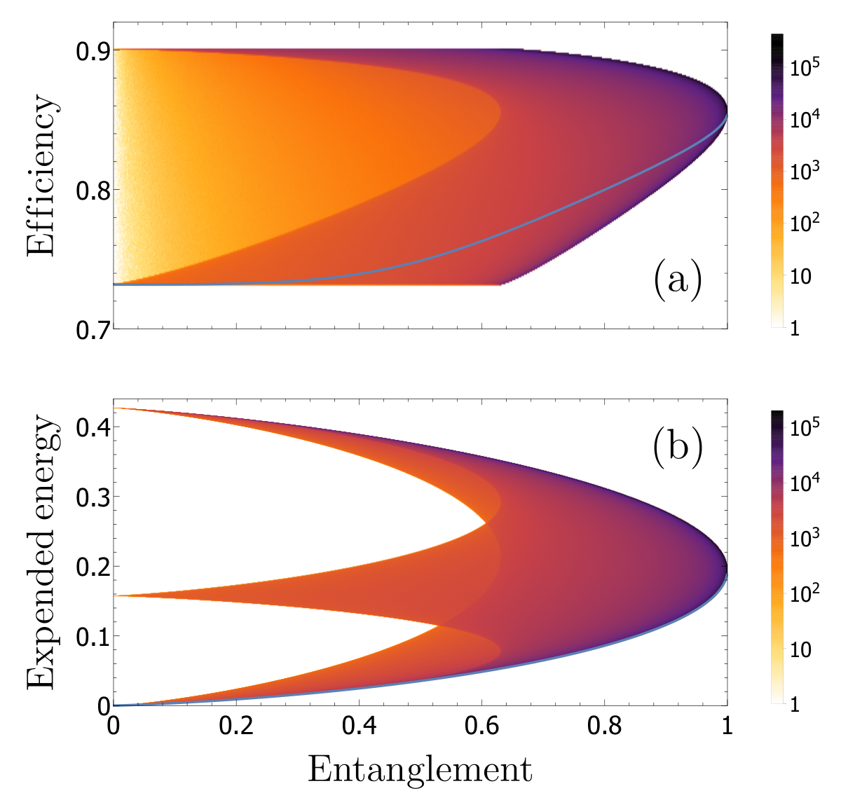
With the interaction Hamiltonian of the modified simple approach of Eq. (24), since [see Eq. (25)], we get an higher efficiency compared to the one we could get by reaching the same states with the nonmodified simple approach. However, the modified simple approach lets us to obtain only states like those of Eq. (6). Figure 2 shows the same two plots of Fig. 1 but using a sample of randomly generated states that can be obtained through the modified simple approach. Indeed, the difference of the sample set is the main responsible for the great difference between the distributions of Fig. 1 and Fig. 2. Even in this case, the MEESs, represented by the blue lines, are not the best ones with respect to the efficiency. Regarding the expended energy, they are still among the cheapest states, but the distribution accumulates on the boundaries contrarily to the case of Fig. 1(b). By zooming enough in the graph, it is possible to see (using a thinner line for the MEESs) that some of the generated states are cheaper than the MEESs. We recall that, in this case only, we were able to find a simple analytical solution of the minimization problem, reported in Appendix B. As in the simple approach case of Fig. 1, the solutions of the minimization problem show, in all systems that we have simulated, that MEESs are very close to the states minimizing the expended energy. We also notice that the maximum value of the efficiency with respect to the normalized entanglement starts to change around . This is probably due to the fact that to obtain a certain degree of entanglement without involving all three states (, and ) is not possible when .

Moving to the results of the unitary approach, Fig. 3 shows the same two plots of Fig. 1 but in the case when the interaction Hamiltonian is obtained through . Notice how the state distribution of Fig. 3 is qualitatively similar to that of Fig. 1. This is due to the fact that the plots in the two figures have been made based on the same kind of sample set. In general, a comparison with all the other figures of this section suggests that the global unitary approach is the less performing.
Figure 4 shows the same plots of previous figures in the case when the interaction is obtained through . As for the modified simple approach, only states with a Schmidt decomposition in the basis can be obtained through this approach [see Eq. (6)]. Indeed, again for this reason, the distribution is completely different with respect to approaches that can give any state as result. In general, the efficiencies are higher compared to the ones obtained with the global approach. This is probably connected to the fact, proved analytically, that when the MSSG and global unitary approaches generate the same state, the MSSG ones are more efficient [see Eq. (36)]. However, even in this case, the MEESs are not among the best ones but they lie very near the lower border of the distribution.


The same plots for the unitary approach on system , reported in Fig. 5, give different results for the efficiency but similar for the expended energy. We can deal with this case by using directly the operator derived in Sec. III.2, even if we did not report explicitly the interaction Hamiltonian needed for implementing the thermalization protocol in Sec. IV.2.2. In this case, for low entanglement, the efficiencies of the MEESs are practically the highest ones. Other simulations suggest that this probably depends on the fact that between the two subsystems and , system is the one with the lowest energy gap between the ground and the first excited state and the highest energy gap between the first and the second excited states. In fact, within the MSSG unitary approaches, the energy spectrum of the local system of interest is more important than the energy spectrum of the other one [see Eq. (35)]. Since for low entanglement, two states in the decomposition are sufficient, we can (heuristically) expect that the weight of the third state has to be marginal. Indeed, considering the spectrum of system and the weights implied by a thermal distribution, the second excited state in MEESs is very low populated for low entanglement, thus leading to high efficiencies. As for the modified simple approach, we can also see in Fig. 4 and 5 that the maximum of the efficiency with respect to the entanglement starts declining roughly at , we think, for the same reasons given in the case of Fig. 2.
Finally, Fig. 6 shows both efficiency and expended energy for all of the analyzed processes but focusing only on the generation of MEESs. Here, we can see that at low entanglement values the most efficient approach to produce a certain MEES is the MSSG unitary approach based on . For higher entanglement values, the best approach seems to be given by the modified simple one. The plots also make clear that the two simple approaches behave the same for MEESs, with the difference originating only from . We also notice that the two MSSG approaches cross at a certain point. This is probably due to the fact the, towards higher entanglement values, the second excited level of both subsystems becomes more important. Therefore, the only positive term in the sum of Eq. (37), i.e., the last one becomes higher. As predicted analytically, the global unitary approach always performs worse than the MSSG ones.
VI Conclusions
In this paper we have proposed several protocols to generate MEESs, i.e., states having the minimum energy for any given amount of entanglement, in a bipartite system made by two noninteracting parts of arbitrary finite dimensions. Some of these protocols are based on the direct use of unitary operators, while the others exploit a zero-temperature thermalization for their realization.
Firstly, we have provided three different unitary operators connecting the ground state of to an arbitrary MEES. While the first operator, , can be decomposed as the product of nonlocal operators, the others, and , can be decomposed as the product of simple two-level local rotations and a local change of phase on a subsystem, and, subsequently, a generalized CNOT gate on the bipartite system. Therefore, the implementation of these unitary transformations in quantum circuits should be easier with respect to the case of .
Secondly, we have identified five different interaction Hamiltonians that, added to the free ones, make possible to generate MEESs by means of a zero-temperature thermalization process. Two of these processes are based on what we have called a simple and a modified simple approach, whereas the others are based on the unitary operators previously identified, , , and .
We have then compared the efficiency of these zero-temperature generation processes as well as the expended energy to run them, both in general and in the case of a specific system, complex enough to unveil the difference between the various protocols. In doing so, we have exploited the relevant fact that our protocols can be also applied to generate states different from the MEESs. In particular, some methods can be used to reach any state of system (with proper modifications when needed), whereas others can only give states the Schmidt decomposition of which is in the basis [cfr. Eq. (6)]. By means of a detailed comparison, we have identified, in the specific system, which are the best-performing protocols. Depending on how much entanglement is required and the spectra of the systems, the better approaches are, in general, one between those based on and , or the modified simple one. Even if the MEESs are not the states minimizing the expended energy to run the generation protocol, we have numerically found, in all systems that we have simulated, that they are very close to them, so that, they are, in general, cheaper to generate than the vast majority of other states. Concerning an experimental implementation of the corresponding interaction Hamiltonians, one can easily find the matrix for all five approaches and realize which is the easiest one to implement.
Appendix A Construction of the unitary operator in the general case
1.
Be a basis for an dimensional Hilbert space and be an arbitrary normalized state with , , and . The following states, together with , form another basis:
| (38) |
where , , and .
Proof.
First we prove that any two states of the set are orthogonal. We start by considering :
| (39) |
Indeed, the same holds for . In the same manner, it is easy to show that . Lastly, we prove that the states are normalized:
| (40) |
∎
We remark that when , .
Theorem 1 lets us write down a unitary operator connecting two arbitrary states. Suppose we want to obtain state from state . As first step, we define the operator
| (41) |
which maps the state to . If , the state (and possibly others) cannot be properly defined since, e.g., . However, we can write the target state with respect to the basis in which and , where is any index value such that , while for , . Accordingly, we write the states of Theorem 1 and the corresponding new with respect to this new basis. Then, before , we apply another unitary operator, , which swaps the states and . In this way, when , we can define as , thus assuring the transition .
By applying the same reasoning to , i.e., , with the proper modification if for the state , , one gets
| (42) |
The transition from to can be obtained in another way, i.e., by exploiting the composition of elementary two-dimensional rotations. We can write
| (43) |
where, for (hereafter we drop the argument to lighten the notation),
| (44) |
while, for ,
| (45) |
To compute the action of we first compute the action of its constituents () for and :
| (46) | ||||
Let us start by studying the action of on the state . By applying the first matrices [i.e., with going from to in Eq. (43)], the amplitude of goes to while that of remains zero. Then, the application of the matrix makes the amplitude of go to and that of from zero to
| (47) |
which is the final amplitude of in the state , and will remain unvaried by the action of the subsequent unitaries with . The application of all unitaries but brings the amplitude of to . Therefore, since correctly changes the phase of , it follows that .
We can also calculate . First, we notice that
| (48) |
since the application of the first matrices make no effect. Then,
| (49) |
This last term can be computed too:
| (50) |
Eventually, we get (also using )
| (51) |
which is equal to Eq. (38). Therefore, we have just shown how the matrix is explicitly decomposable as a product of elementary two-dimensional rotations, i.e., .
Appendix B Minimization of the expended energy in the modified simple thermalization protocol
Here, we show how to find the states minimizing for a fixed entanglement in the modified simple approach of Sec. IV.1 using the interaction Hamiltonian of Eq. (24). Since this Hamiltonian can only generate states belonging to the subspace generated by the kets , any target state has the form of Eq. (6). Therefore, we can rewrite the formula of [cfr. Eq. (26)] as follows (setting for simplicity of notation):
| (52) |
The minimization problem can be now easily solved by considering the coefficients as the coefficients of a thermal state with respect to a fictitious Hamiltonian with eigenvalues and (see also Sec. I and Sec. II of the Supplemental Material of Ref. Piccione et al. 2020). By doing so we get
| (53) |
where is obtained by requiring that
| (54) |
Appendix C Construction of the interaction matrix obtained through a unitary transformation
In the zero-temperature limit, dissipation can be used to generate pure states. If a system is described by a Hamiltonian with a nondegenerate lowest eigenvalue, dissipation due to the interaction with a zero-temperature bath will generally lead to the ground state of the system Breuer and Petruccione 2007. Let us call an eigenbasis for . For any desired state (for simplicity, we only consider states with ), by using a proper unitary operator defined as in Eq. (41), it is possible to write an Hermitian operator such that is the ground state of :
| (55) |
where runs over all the eigenvalues of , i.e., with respect to the notation of Sec. II, is a shorthand for all combinations of , for all and , and with . Writing (we drop the explicit dependence on to lighten the notation), we obtain
| (56) |
We can explicitly find the coefficients of the Hamiltonian by calculating [cfr. Eq. (41)]. For , using Eq. (38), we get:
| (57) |
Let us start from the diagonal elements. For we get
| (58) |
while for we have
| (59) |
Since is an Hermitian matrix, it suffices to continue the calculations by analyzing the case. For we get
| (60) |
whereas for we have
| (61) |
Appendix D Efficiency and expended energy for the global unitary approach
In this Appendix, we obtain the general formulas for the efficiency and expended energy of the global unitary approach by using their definition of Eq. (20).
By using Eqs. (55), (56), and (57) in Eq. (20), we get
| (62) |
If we set , which can always be done by adding a constant term to , we get
| (63) |
which makes clear that , as it should be. When considering target states like those of Eq. (6), the efficiency of Eq. (63) and the denominator therein appearing become, respectively, the efficiency and the energy expense reported in Eq. (31).
Now, we prove that [see Eq. (20)] cannot be higher than in the global unitary approach:
| (64) |
where the last inequality comes from the invariance of the spectrum for unitary transformations.
Appendix E Efficiency and expended energy in the MSSG unitary approaches
Here, we want to calculate the quantities of Eq. (20) in the case of the states obtainable within the MSSG unitary approaches, i.e., states of the form of Eq. (6). In these approaches, a state is obtained by applying or to and then the corresponding generalized CNOT gate [see Eqs. (18) and (19)] is applied to the resulting state on system . Let us focus on the case, where
| (65) |
First, we notice that . Therefore, using also Eqs. (13) and (57) applied to the calculation of , we obtain
| (66) |
Then, we calculate
| (67) |
Eventually, the expended energy in this case is equal to
| (68) |
Now, we show that the expended energy within the global approach is higher that in the MSSG unitary approaches when they generate the same state . The expended energy in the global approach can be written as [cfr. Eq. (62) applied to a state ]
| (69) |
and the difference between and is equal to
| (70) |
Since we can set without changing the above quantity, we conclude that the MSSG version of the protocol based on always performs better than the global one. The derivation of is similar since, analogously to the previous case, , and leads to the same expression of Eq. (68) with the quantities and swapped between them.
To complete the analysis we also write the difference regarding the expended energy in the two MSSG approaches:
| (71) |
In this case, which approach is better depends both on the target state and the spectra of and .
Appendix F Explicit calculations for two qubits
In this Appendix, we explicitly calculate the three unitary transformations proposed in Sec. III and the interaction Hamiltonians proposed in Sec. IV for the archetypical example of a bipartite system composed of two qubits, having as free Hamiltonians
| (72) |
where is the -Pauli matrix of qubit (). As basis for we use , where, for each qubit, and . Let us define , then the MEES for a two qubit system, as reported in Piccione et al. 2020, and considering arbitrary phases, is given by
| (73) |
where .
Starting from Eqs. (8), (13), (18), and (19) [ is defined analogously to what done in Eq. (13)], straightforward calculations give for , , and :
| (74) |
| (75) |
and
| (76) |
We can see, explicitly, that the three unitary operators proposed in Sec. III are different.
Regarding the thermalization approach, we can immediately write down the interaction Hamiltonian obtained through the simple approach:
| (77) |
where and . For comparison, the modified simple approach leads to
| (78) |
which lacks the diagonal terms et .
Turning to the zero-temperature approach based on the global unitary transformation, the use of leads to
| (79) |
Even if this Hamiltonian is similar to that of Eq. (78), it is not the same one. This was predictable since the modified simple approach changes the spectrum of whereas all unitary ones do not. Moreover, it does not exist a number such that so that the two Hamiltonians cannot describe the same physics even with a rescaling of the energy.
Moving to the MSSG thermalization approaches, the use of leads to
| (80) |
whereas the use of to
| (81) |
Since all of these interaction Hamiltonians are different (even considering rescaling), we can conclude that the five methods give rise to physically different interactions.
In Ref. Piccione et al. 2020 the following interaction Hamiltonian was proposed to make the ground state
| (82) |
where are Pauli operators on system with . The matrix structure of this operator is
| (83) |
which lacks the diagonal terms present in all the general approaches we provided. Therefore, the methods that we presented in this paper cannot be used to obtain this empirical Hamiltonian that we found by hand in Ref. Piccione et al. 2020.
References
- Einstein et al. (1935) A. Einstein, B. Podolsky, and N. Rosen, Can Quantum-Mechanical Description of Physical Reality Be Considered Complete?, Phys. Rev. 47, 777 (1935).
- Bell (1964) J. S. Bell, On the Einstein Podolsky Rosen paradox, Phys. Phys. Fiz. 1, 195 (1964).
- Horodecki et al. (2009) R. Horodecki, P. Horodecki, M. Horodecki, and K. Horodecki, Quantum entanglement, Rev. Mod. Phys. 81, 865 (2009).
- Nielsen and Chuang (2010) M. A. Nielsen and I. L. Chuang, Quantum Computation and Quantum Information: 10th Anniversary Edition (Cambridge University Press, 2010).
- Plenio et al. (1999) M. B. Plenio, S. F. Huelga, A. Beige, and P. L. Knight, Cavity-loss-induced generation of entangled atoms, Phys. Rev. A 59, 2468 (1999).
- Braun (2002) D. Braun, Creation of entanglement by interaction with a common heat bath, Phys. Rev. Lett. 89, 277901 (2002).
- Bellomo et al. (2008) B. Bellomo, R. Lo Franco, S. Maniscalco, and G. Compagno, Entanglement trapping in structured environments, Phys. Rev. A 78, 060302(R) (2008).
- Sarlette et al. (2011) A. Sarlette, J. M. Raimond, M. Brune, and P. Rouchon, Stabilization of Nonclassical States of the Radiation Field in a Cavity by Reservoir Engineering, Phys. Rev. Lett. 107, 010402 (2011).
- Krauter et al. (2011) H. Krauter, C. A. Muschik, K. Jensen, W. Wasilewski, J. M. Petersen, J. I. Cirac, and E. S. Polzik, Entanglement Generated by Dissipation and Steady State Entanglement of Two Macroscopic Objects, Phys. Rev. Lett. 107, 080503 (2011).
- Bellomo and Antezza (2013) B. Bellomo and M. Antezza, Steady entanglement out of thermal equilibrium, Europhys. Lett. 104, 10006 (2013).
- Bellomo and Antezza (2015) B. Bellomo and M. Antezza, Nonequilibrium dissipation-driven steady many-body entanglement, Phys. Rev. A 91, 042124 (2015).
- Bellomo et al. (2017) B. Bellomo, R. Lo Franco, and G. Compagno, N identical particles and one particle to entangle them all, Phys. Rev. A 96, 022319 (2017).
- Luo et al. (2017) X.-Y. Luo, Y.-Q. Zou, L.-N. Wu, Q. Liu, M.-F. Han, M. K. Tey, and L. You, Deterministic entanglement generation from driving through quantum phase transitions, Science 355, 620 (2017).
- Çakmak et al. (2019) B. Çakmak, S. Campbell, B. Vacchini, Ö. E. Müstecaplıoğlu, and M. Paternostro, Robust multipartite entanglement generation via a collision model, Phys. Rev. A 99, 012319 (2019).
- Goldberg and James (2019) A. Z. Goldberg and D. F. V. James, Entanglement generation via diffraction, Phys. Rev. A 100, 042332 (2019).
- Castellini et al. (2019) A. Castellini, B. Bellomo, G. Compagno, and R. Lo Franco, Activating remote entanglement in a quantum network by local counting of identical particles, Phys. Rev. A 99, 062322 (2019).
- Egger et al. (2019) D. J. Egger, M. Ganzhorn, G. Salis, A. Fuhrer, P. Müller, P. Kl. Barkoutsos, N. Moll, I. Tavernelli, and S. Filipp, Entanglement Generation in Superconducting Qubits Using Holonomic Operations, Phys. Rev. Applied 11, 014017 (2019).
- Katz et al. (2020) O. Katz, R. Shaham, E. S. Polzik, and O. Firstenberg, Long-lived Entanglement Generation of Nuclear Spins Using Coherent Light, Phys. Rev. Lett. 124, 043602 (2020).
- Xi et al. (2019) Y. Xi, T. Zhang, Z.-J. Zheng, X. Li-Jost, and S.-M. Fei, Converting quantum coherence to genuine multipartite entanglement and nonlocality, Phys. Rev. A 100, 022310 (2019).
- Korzekwa et al. (2019) K. Korzekwa, C. T. Chubb, and M. Tomamichel, Avoiding Irreversibility: Engineering Resonant Conversions of Quantum Resources, Phys. Rev. Lett. 122, 110403 (2019).
- Piccione et al. (2020) N. Piccione, B. Militello, A. Napoli, and B. Bellomo, Energy bounds for entangled states, Phys. Rev. Research 2, 022057(R) (2020).
- Ikonen et al. (2017) J. Ikonen, J. Salmilehto, and M. Möttönen, Energy-efficient quantum computing, npj Quantum Inf. 3, 17 (2017).
- Bakhshinezhad et al. (2019) F. Bakhshinezhad, F. Clivaz, G. Vitagliano, P. Erker, A. Rezakhani, M. Huber, and N. Friis, Thermodynamically optimal creation of correlations, J. Phys. A Math. Theor. 52, 465303 (2019).
- Galve and Lutz (2009) F. Galve and E. Lutz, Energy cost and optimal entanglement production in harmonic chains, Phys. Rev. A 79, 032327 (2009).
- Bény et al. (2018) C. Bény, C. T. Chubb, T. Farrelly, and T. J. Osborne, Energy cost of entanglement extraction in complex quantum systems, Nat. Commun. 9, 3792 (2018).
- Hackl and Jonsson (2019) L. Hackl and R. H. Jonsson, Minimal energy cost of entanglement extraction, Quantum 3, 165 (2019).
- Piccione et al. (2019) N. Piccione, B. Militello, A. Napoli, and B. Bellomo, Simple scheme for extracting work with a single bath, Phys. Rev. E 100, 032143 (2019).
- Bechmann-Pasquinucci and Peres (2000) H. Bechmann-Pasquinucci and A. Peres, Quantum Cryptography with 3-State Systems, Phys. Rev. Lett. 85, 3313 (2000).
- Bullock et al. (2005) S. S. Bullock, D. P. O’Leary, and G. K. Brennen, Asymptotically Optimal Quantum Circuits for -Level Systems, Phys. Rev. Lett. 94, 230502 (2005).
- Lanyon et al. (2009) B. P. Lanyon, M. Barbieri, M. P. Almeida, T. Jennewein, T. C. Ralph, K. J. Resch, G. J. Pryde, J. L. O’Brien, A. Gilchrist, and A. G. White, Simplifying quantum logic using higher-dimensional Hilbert spaces, Nat. Phys. 5, 134 (2009).
- Yan et al. (2019) X.-Y. Yan, N.-R. Zhou, L.-H. Gong, Y.-Q. Wang, and X.-J. Wen, High-dimensional quantum key distribution based on qudits transmission with quantum Fourier transform, Quantum Inf. Process. 18, 271 (2019).
- Kiktenko et al. (2020) E. O. Kiktenko, A. S. Nikolaeva, P. Xu, G. V. Shlyapnikov, and A. K. Fedorov, Scalable quantum computing with qudits on a graph, Phys. Rev. A 101, 022304 (2020).
- Godfrin et al. (2017) C. Godfrin, A. Ferhat, R. Ballou, S. Klyatskaya, M. Ruben, W. Wernsdorfer, and F. Balestro, Operating Quantum States in Single Magnetic Molecules: Implementation of Grover’s Quantum Algorithm, Phys. Rev. Lett. 119, 187702 (2017).
- Blok et al. (2021) M. S. Blok, V. V. Ramasesh, T. Schuster, K. O’Brien, J. M. Kreikebaum, D. Dahlen, A. Morvan, B. Yoshida, N. Y. Yao, and I. Siddiqi, Quantum Information Scrambling on a Superconducting Qutrit Processor, Phys. Rev. X 11, 021010 (2021).
- Kues et al. (2017) M. Kues, C. Reimer, P. Roztocki, L. R. Cortés, S. Sciara, B. Wetzel, Y. Zhang, A. Cino, S. T. Chu, B. E. Little, et al., On-chip generation of high-dimensional entangled quantum states and their coherent control, Nature (London) 546, 622 (2017).
- Reimer et al. (2019) C. Reimer, S. Sciara, P. Roztocki, M. Islam, L. R. Cortés, Y. Zhang, B. Fischer, S. Loranger, R. Kashyap, A. Cino, et al., High-dimensional one-way quantum processing implemented on -level cluster states, Nat. Phys. 15, 148 (2019).
- Imany et al. (2019) P. Imany, J. A. Jaramillo-Villegas, M. S. Alshaykh, J. M. Lukens, O. D. Odele, A. J. Moore, D. E. Leaird, M. Qi, and A. M. Weiner, High-dimensional optical quantum logic in large operational spaces, npj Quantum Inf. 5, 59 (2019).
- Wilmott (2011) C. Wilmott, On swapping the states of two qudits, Int. J. Quantum Inf. 09, 1511 (2011).
- Gao et al. (2019) X. Gao, M. Krenn, J. Kysela, and A. Zeilinger, Arbitrary -dimensional Pauli gates of a flying qudit, Phys. Rev. A 99, 023825 (2019).
- Isdrailă et al. (2019) T.-A. Isdrailă, C. Kusko, and R. Ionicioiu, Cyclic permutations for qudits in dimensions, Sci. Rep. 9, 6337 (2019).
- Low et al. (2020) P. J. Low, B. M. White, A. A. Cox, M. L. Day, and C. Senko, Practical trapped-ion protocols for universal qudit-based quantum computing, Phys. Rev. Research 2, 033128 (2020).
- Vidal (2000) G. Vidal, Entanglement monotones, J. Mod. Opt. 47, 355 (2000).
- Plenio and Virmani (2007) M. B. Plenio and S. Virmani, An introduction to Entanglement Measures, Quantum Inf. Comput. 7, 1 (2007).
- (44) The states which have zero projection on can indeed be obtained by means of simple modifications of the method. See the relevant discussion in Appendix A.
- (45) In Ref. Wilmott 2011 the CNOT gate is given for a bipartite system composed of two qubits with the same dimensions. Here, we have used what seemed to us the most natural extension of the CNOT gate operator, i.e., using system as a qudit of dimension . Therefore, we apply the CNOT gate such that it involves only the first levels of both systems.
- (46) Indeed, the operator acts as on the first levels of system , while leaving unvaried the others.
- Breuer and Petruccione (2007) H.-P. Breuer and F. Petruccione, The Theory of Open Quantum Systems (Oxford University Press, New York, 2007).