Off-Policy Evaluation of Bandit Algorithm from Dependent Samples under Batch Update Policy
Abstract
The goal of off-policy evaluation (OPE) is to evaluate a new policy using historical data obtained via a behavior policy. However, because the contextual bandit algorithm updates the policy based on past observations, the samples are not independent and identically distributed (i.i.d.). This paper tackles this problem by constructing an estimator from a martingale difference sequence (MDS) for the dependent samples. In the data-generating process, we do not assume the convergence of the policy, but the policy uses the same conditional probability of choosing an action during a certain period. Then, we derive an asymptotically normal estimator of the value of an evaluation policy. As another advantage of our method, the batch-based approach simultaneously solves deficient support problem. Using benchmark and real-world datasets, we experimentally confirm the effectiveness of the proposed method.
1 Introduction
As an instance of sequential decision-making problems, the multi-armed bandit (MAB) algorithms have attracted significant attention in various applications, such as ad optimization, personalized medicine, search engines, and recommendation systems. Recently, various methods for evaluating a new policy using historical data obtained via the MAB algorithms (Beygelzimer & Langford 2009; Li et al. 2010) have emerged. The goal of off-policy evaluation (OPE) is to evaluate a new policy by estimating the expected reward obtained from the new policy (Dudík et al. 2011; Wang et al. 2017; Narita et al. 2019; Bibaut et al. 2019; Kallus & Uehara 2019; Oberst & Sontag 2019). Although an OPE algorithm estimates the expected reward from a new policy, most existing studies presume that the samples are independent and identically distributed (i.i.d.). However, the MAB algorithm policy updates the probability of choosing an action based on past observations, and samples are not i.i.d. owing to this update. In this case, such existing studies do not guarantee that their estimators have asymptotic normality and -consistency for a sample size . Therefore, there is a strong motivation to establish a novel method for OPE from dependent samples.
Several pioneering studies address OPE from dependent samples (van der Laan 2008; Hahn et al. 2011; van der Laan & Lendle 2014; Luedtke & van der Laan 2016; Hadad et al. 2019; Kato et al. 2020a). We can group the methods for deriving asymptotic normality into the following three groups: (a) van der Laan 2008, van der Laan & Lendle 2014, Hadad et al. 2019, and Kato et al. 2020a derive the asymptotic normality with the central limit theorem (CLT) of a martingale difference sequence (MDS) by assuming that the probability of choosing an action converges to a time-invariant probability; (b) Luedtke & van der Laan 2016 derives the asymptotic normality by standardizing a MDS, which is also used in the first group; (c) Hahn et al. 2011 apply asymptotic theory for the batched probability update process.
This paper focuses on an approach of the third group; that is, there are sufficiently large sample sizes in each batch. Compared with Hahn et al. 2011, our proposed method is more general and applicable in practical applications. Our method has the following three advantages compared with existing studies: (i) it does not assume convergence of the probability of choosing an action; (ii) it allows the probability of choosing an action to be for some actions in some batches; (iii) we can also use non-Donsker nuisance estimators as well as van der Laan & Lendle 2014.
This paper has three main contributions. First, we provide a solution for OPE from dependent samples obtained via the MAB algorithms. Second, under the batch update policy, the proposed estimator achieves the asymptotic normality with fewer assumptions. Third, the estimator also experimentally shows a lower mean squared error (MSE) in some cases.
2 Problem Setting
Here, we formulate OPE under a batch update.
2.1 Date-Generating Process
Let be an action taking variable in , the covariate observed by the decision maker when choosing an action , and the space of covariate. Let us denote a random variable of a reward at period as , where is a potential outcome11 1 We can express the DGP without using the potential outcome variable (Kato et al. 2020b).. In this paper, we have access to a dataset with the following data-generating process (DGP):
| (1) |
where denotes the history until period defined as with the space , denotes the density of the covariate , denotes the probability of choosing an action conditioned on and , and denotes the density of an outcome conditioned on and . We assume that and are invariant across periods, but can take different values across periods. Let us call a policy inducing a behavior policy.
2.2 Off-Policy Evaluation
This paper considers estimating the value of an evaluation policy using samples obtained under the behavior policy. Let an evaluation policy be a probability of choosing an action conditioned on a covariate . We are interested in estimating the expected reward from any pre-specified evaluation policy . Then, we define the expected reward under an evaluation policy as . For brevity, we also denote as . The goal of this paper is to estimate using dependent samples under a batch update policy. To identify , we assume overlaps in policy and the boundedness of the outcome.
Assumption 1.
There exists a constant such that .
Assumption 2.
There exists a constant such that .
Remark 1 (Existing Methods for OPE).
We review three types of standard estimators of under the case where in the DGP defined in (1). The first estimator is an inverse probability weighting (IPW) estimator given by (Rubin 1987; Hirano et al. 2003; Swaminathan & Joachims 2015). Although this estimator is unbiased when the behavior policy is known, it suffers from high variance. The second estimator is a direct method (DM) estimator , where is an estimator of (Hahn 1998). This estimator is known to be weak against model misspecification for . The third estimator is an augmented IPW (AIPW) defined as (Robins et al. 1994; Chernozhukov et al. 2018). Under certain conditions, it is known that this estimator achieves the efficiency bound (a.k.a semiparametric lower bound), which is the lower bound of the asymptotic MSE of OPE among regular -consistent estimators (van der Vaart 1998).
Remark 2 (Semiparametric Lower Bound).
The lower bound of the variance is defined for an estimator of under some posited models of the DGP. If this posited model is a parametric model, it is equal to the Cramér-Rao lower bound. When this posited model is a semiparametric model, we can define a corresponding Cramér-Rao lower bound Bickel et al. 1998. Narita et al. 2019 gives the semiparametric lower bound of the DGP (1) under as .
Notations:
Let us denote and as and , respectively. Let be the class of . Let be an estimator of constructed from , respectively. Let be the normal distribution with the mean and the variance . For a random variable and function , let be the -norm.
2.3 Patterns of Probability Update
In this paper, based on the update of , we classify the policies into two patterns, sequential update policy and batch update policy. For the sequential update policy, the policy updates at each period (van der Laan 2008; van der Laan & Lendle 2014; Kato et al. 2020a). Under the batch update policy, after the policy continues using a fixed probability for some periods without updates, the policy updates (Hahn et al. 2011; Narita et al. 2019). Although the sequential update is standard in the MAB problem, we often apply batch updates in industrial applications such as ad-optimization (Narita et al. 2019). For OPE under the sequential update, van der Laan 2008, van der Laan & Lendle 2014, Luedtke & van der Laan 2016, Hadad et al. 2019, and Kato et al. 2020a proposed estimators with the asymptotic normality. For instance, an adaptive AIPW (A2IPW) estimator (van der Laan & Lendle 2014; Hadad et al. 2019; Kato et al. 2020a) has asymptotic normality if the behavior policy converges. On the other hand, we consider OPE under a batch update. Let denote the number of updates and denotes the batch index. For , the probability is updated at a period , where , using samples , where and . Thus, in addition to the DGP (1), we assume
where denotes the assignment probability updated based on samples until the period .
2.4 Related Work
For the sequential update, van der Laan 2008, van der Laan & Lendle 2014, Hadad et al. 2019, and Kato et al. 2020a assume that the probability of choosing an action converges to a time-invariant function almost certainly; that is, , where . This assumption enables us to apply the CLT for MDS. van der Laan & Lendle 2014 proposed constructing step-wise nuisance estimators, which enables us to derive asymptotic normality without Donsker’s conditions of nuisance estimators. This technique is a generalization of sample-splitting, which is also called cross-fitting in a context of double/debiased machine learning (Klaassen 1987; Zheng & van der Laan 2011; Chernozhukov et al. 2018). For the A2IPW estimator, Hadad et al. 2019 proposed using an adaptive weight for stabilizing the behavior, and Kato et al. 2020a derived concentration inequality based on the law of iterated logarithms. On the other hand, we also construct an MDS and apply the CLT, but do not assume by using batch update policy. Instead, we assume a sufficient sample size for each batch.
For such a non-stationary setting, Luedtke & van der Laan 2016 also proposed an estimator with asymptotically normality for sequential update policy without using batch update policy. For deriving the asymptotic normality, Luedtke & van der Laan 2016 used standardization for an MDS. Although the method enables us to construct an asymptotically normal estimator for various estimators, the proposed estimator only has -consistency for another sample size , not , to estimate the variances of the MDS.
As other related work, in the MAB problem, Perchet et al. 2016 considered the setting of batch policy updates. In OPE, Narita et al. 2019 also discuss a similar problem setting, but they assume that samples are i.i.d. Independently, Zhang et al. 2020 provided a method for deriving a confidence interval of an ordinary least squares estimator, which is a different parameter of what we want to estimate.
3 OPE under Batch Update Policy
This section introduces a concept for conducting OPE under the batch update policy and a method based on the concept with its theoretical properties.
3.1 Strategy for OPE
For OPE under batch update policy, we consider asymptotic properties based on the assumption of as for fixed . Because is i.i.d., we can use the standard limit theorems for the partial sum of the samples to obtain an asymptotically normal estimator of . However, we also have the motivation to use all samples together to increase the efficiency of the estimator. Therefore, based on the idea of generalized method of moments (GMM), we propose an estimator of considering the sample averages of each block as an empirical moment conditions. The main difference from the standard GMM is the assumption that the samples are not i.i.d. However, for the case under the batch update, we can apply the central limit theorems (CLT) for the martingale difference sequences (MDS) by appropriately constructing an estimator. We describe the proposed method as follows.
3.2 Estimator for OPE
We propose an estimator of based on a idea of GMM. For an index of batch , a function such that and an evaluation policy , we define as , where and
Let us note that, for , , , and , the sequence is an MDS: for , by , we have
Let us also define
Then, the sequence is an MDS with respect to ; that is, . Using the sequence , we define an estimator of OPE as
| (2) |
where and is a data-dependent -dimensional positive semi-definite matrix. Let us note that the estimator defined in Eq. (2) is an application of GMM with the moment condition . For the minimization problem defined in Eq. (2), we can analytically calculate the minimizer as , where is an -dimensional vector such that , and is
We call the estimator a Batch-based Adaptive AIPW (BA2IPW) estimator. In Appendix B, we discuss the GMM perspective in more detail.
3.3 Asymptotic Properties
Here, we show the consistency and asymptotic normality of the proposed BA2IPW estimator .
Theorem 1 (Consistency of the BA2IPW Estimator).
Proof.
Theorem 2 (Asymptotic Distribution of the BA2IPW Estimator).
The proof is shown in Appendix C. Readers might consider that the use of MDS for deriving the asymptotic normality is unnecessary. We discuss the necessity of MDS in Appendix D. We can also define a corresponding Batch-based Adaptive IPW (BAdaIPW). For the BAdaIPW estimator, the variance of a batch is .
Remark 3 (Construction of and Donsker Condition).
As well as the cross-fitting of double/debiased machine learning proposed by Klaassen 1987,Zheng & van der Laan 2011,van der Laan & Lendle 2014, and Chernozhukov et al. 2018, the proposed estimator does not require Donsker’s condition for asymptotic normality. This property comes from the MDS as pointed by van der Laan & Lendle 2014. On the other hand, because the samples are not independent, we cannot use the standard regression to obtain a consistent estimator of . For example, Yang & Zhu 2002 propose a nonparametric method for the bandit process under some mild conditions.
3.4 Weight of the Proposed Estimator
Next, we discuss the choice of weight .
Equal Weight:
A naive choice is weighting the moment conditions equality; that is, . In this case, the proposed estimator boils down to , which is almost the same as the A2IPW estimator. Although the estimator itself is similar to the A2IPW estimator, the theoretical guarantee for the asymptotic normality is different. While the A2IPW estimator uses the assumption that the policy converges to a time-invariant policy, the proposed BA2IPW estimator uses the assumption of the batch update. We call the BA2IPW estimator with the equal weight a Plain BA2IPW (PBA2IPW) estimator.
Efficient Weight:
First, we consider an efficient weight that minimizes the asymptotic variance of . As well as the standard GMM, the -th element of the efficient weight is given as (Hamilton 1994). Here, we use the orthogonality among moment conditions; that is, zero covariance. In this case, the asymptotic variance becomes . Therefore, for gaining efficiency, we use a weight , where is an estimator of . We call the BA2IPW estimator with the efficient weight an Efficient BA2IPW (EBA2IPW) estimator.
Remark 4 (Estimation of ).
If , we also have from the continuous mapping theorem. In this paper, we propose two estimators defined as and .
Weight for Numerical Stability:
As explained above, we can obtain an efficient weight that minimizes the asymptotic variance. However, as Hadad et al. 2019 pointed out, when using time-variance estimators , early variable might be unstable due to the existence of an inaccurate estimators at early stages. Hadad et al. 2019 proposed an adaptive weight that puts more weight on later variables in the estimator. In our problem setting, we can also introduce such weights. However, unlike the adaptive weight proposed by Hadad et al. 2019, which must be martingale, we do not require martingales on the weights. This property is a benefit of the batch update. For instance, for stabilization, we define a weight , where and is a constant. The first term is an efficient weight described above. The second term reflects the deviation between and , which would be more accurate because it uses more samples.
3.5 Main Algorithm
As discussed in Section 3.4, we can minimize the asymptotic variance of the proposed estimator by choosing appropriately. However, to obtain , which is the optimal weight that minimizes the asymptotic variance, we need a consistent estimator of , which is what we want to estimate. On the other hand, we have a consistent estimator of without using an optimal weight matrix . Based on these properties, we propose two-step estimation. First, using an arbitrary positive definite weight , such as the identity matrix, we obtain an initial estimate . Then, using , we construct . We can obtain an efficient estimator of , as discussed. More generally, we consider an algorithm with iteration such that after obtaining , we estimate and obtain a next estimator by using . We refer to this algorithm with -iterations as -step BA2IPW estimation. We can use sufficiently large because, at each iteration, we only calculate the weighted average of the moment conditions using , which is not time-consuming. Although the asymptotic properties of the iterated estimator are the same as those of the two-step estimator, we report that the iteration improves the empirical performance in some cases. For , we summarize the -Step BA2IPW Estimation in Algorithm 1. We can use any method to construct and as long as they are consistent for bandit data and satisfy some regularity conditions needed for Theorem 4.
4 Deficient Support Problem
As an application of BA2IPW, we consider an OPE without Assumption 1, which assumes that there exists such that . Instead of Assumption 3, we consider a situation in which we are allowed to change the support of actions in each batch. For example, in the first batch, we choose an action from a set with a probability larger than , but we choose an action from a set with a probability larger than in the second batch. In this case, the probability of choosing the action is in the first batch, while the probability of choosing the action is in the second batch. This situation is a common in practice and called deficient support problem (Sachdeva et al. 2020). For this problem, instead of Assumption 1, we use the following assumption.
Assumption 3.
For , there exist and such that .
Under this assumption, if for at least one batch, we are allowed to use for . With this assumption, we derive the asymptotic normality in Appendix E. Thus, our approach provides a new solution to this problem.
| Datasets | satimage | pendigits | mnist | letter | sensorless | connect-4 | ||||||
|---|---|---|---|---|---|---|---|---|---|---|---|---|
| Metrics | MSE | SD | MSE | SD | MSE | SD | MSE | SD | MSE | SD | MSE | SD |
| PBA2IPW | 0.038 | 0.002 | 0.129 | 0.047 | 0.173 | 0.104 | 0.331 | 0.547 | 0.146 | 0.089 | 0.021 | 0.021 |
| EBA2IPW | 0.050 | 0.006 | 0.190 | 0.030 | 0.191 | 0.025 | 0.398 | 0.062 | 0.182 | 0.028 | 0.025 | 0.022 |
| EBA2IPW’ | 0.044 | 0.003 | 0.182 | 0.029 | 0.102 | 0.012 | 0.389 | 0.064 | 0.177 | 0.027 | 0.025 | 0.024 |
| BAdaIPW | 0.077 | 0.010 | 0.178 | 0.082 | 0.200 | 0.111 | 0.333 | 0.537 | 0.160 | 0.093 | 0.027 | 0.027 |
| AdaDM | 0.141 | 0.010 | 0.493 | 0.034 | 0.434 | 0.036 | 0.476 | 0.023 | 0.413 | 0.031 | 0.142 | 0.024 |
| AIPW | 0.032 | 0.001 | 0.110 | 0.030 | 0.244 | 0.028 | 0.254 | 0.216 | 0.128 | 0.064 | 0.055 | 0.022 |
| DM | 0.099 | 0.004 | 0.452 | 0.025 | 0.282 | 0.028 | 0.459 | 0.023 | 0.395 | 0.025 | 0.086 | 0.018 |
| Datasets | satimage | pendigits | mnist | letter | sensorless | connect-4 | ||||||
|---|---|---|---|---|---|---|---|---|---|---|---|---|
| Metrics | MSE | SD | MSE | SD | MSE | SD | MSE | SD | MSE | SD | MSE | SD |
| PBA2IPW | 0.050 | 0.005 | 0.088 | 0.015 | 0.240 | 0.415 | 0.205 | 0.088 | 0.162 | 0.057 | 0.032 | 0.032 |
| EBA2IPW | 0.014 | 0.000 | 0.029 | 0.002 | 0.240 | 0.070 | 0.434 | 0.036 | 0.239 | 0.054 | 0.030 | 0.022 |
| EBA2IPW’ | 0.036 | 0.005 | 0.081 | 0.017 | 0.142 | 0.030 | 0.422 | 0.032 | 0.202 | 0.038 | 0.037 | 0.033 |
| BAdaIPW | 0.087 | 0.037 | 0.122 | 0.030 | 0.275 | 0.406 | 0.219 | 0.090 | 0.183 | 0.067 | 0.057 | 0.057 |
| AdaDM | 0.076 | 0.002 | 0.230 | 0.008 | 0.372 | 0.020 | 0.451 | 0.018 | 0.327 | 0.021 | 0.071 | 0.023 |
| AIPW | 0.036 | 0.003 | 0.058 | 0.012 | 0.136 | 0.007 | 0.170 | 0.043 | 0.134 | 0.038 | 0.022 | 0.012 |
| DM | 0.009 | 0.000 | 0.049 | 0.001 | 0.161 | 0.008 | 0.371 | 0.019 | 0.214 | 0.013 | 0.019 | 0.010 |
5 Estimation of the Behavior Policy
In the proposed BA2IPW method, we assume that the true behavior policy is known. However, in many real-world applications, the assumption does not hold. To solve this problem, by using an estimator of , which is constructed from as well as , we also propose a Batch-based Adaptive Doubly Robust (BADR) as , where is an -dimensional vector such that ,
and
For the BADR estimator, we show the asymptotic normality as follows. The proof is shown in Appendix F.
6 Off-Policy Learning
An important application of OPE is Off-Policy Learning (OPL), which attempts to determine the optimal policy maximizing the expected reward. Let us define the optimal policy as , where is a policy class. By applying each OPE estimator, we estimate the optimal policy as .
|
| Datasets | satimage | pendigits | mnist | letter | sensorless | connect-4 | ||||||
|---|---|---|---|---|---|---|---|---|---|---|---|---|
| Metrics | RWD | SD | RWD | SD | RWD | SD | RWD | SD | RWD | SD | RWD | SD |
| PBA2IPW | 0.812 | 0.020 | 0.690 | 0.072 | 0.493 | 0.298 | 0.172 | 0.090 | 0.264 | 0.131 | 0.665 | 0.030 |
| EBA2IPW | 0.813 | 0.022 | 0.717 | 0.063 | 0.519 | 0.313 | 0.135 | 0.073 | 0.289 | 0.126 | 0.679 | 0.024 |
| BAdaIPW | 0.815 | 0.023 | 0.697 | 0.089 | 0.515 | 0.312 | 0.150 | 0.078 | 0.313 | 0.145 | 0.677 | 0.024 |
| AdaDM | 0.777 | 0.033 | 0.478 | 0.076 | 0.191 | 0.151 | 0.046 | 0.026 | 0.190 | 0.091 | 0.654 | 0.023 |
| AIPW | 0.819 | 0.020 | 0.698 | 0.062 | 0.515 | 0.312 | 0.154 | 0.087 | 0.287 | 0.141 | 0.678 | 0.024 |
| DM | 0.791 | 0.034 | 0.544 | 0.071 | 0.247 | 0.174 | 0.057 | 0.036 | 0.210 | 0.090 | 0.654 | 0.023 |
7 Experiments
Using benchmark datasets and real-world logged data, we demonstrate the effectiveness of the BA2IPW estimator with an equal weight (PBA2IPW) and efficient weight using variance estimators (EBA2IPW) and (EBA2IPW’), and BAdaIPW estimator with an equal weight (BAdaIPW). Note that although the forms of the several estimators are the same as the existing studies, the theoretical guarantees are different.
7.1 Experiments with Benchmark Dataset
Following Dudík et al. 2011 and Farajtabar et al. 2018, we evaluate the proposed estimators using classification datasets by transforming them into contextual bandit data. From the LIBSVM repository, we use the satimage, pendigits, mnist, letter, sensorless, and connect-4 datasets 22 2 https://www.csie.ntu.edu.tw/~cjlin/libsvmtools/datasets/. For a batched update behavior policy, we use the random walk (RW) and LinearUCB (UCB) (Sutton & Barto 1998; Li et al. 2010; Chu et al. 2011) policies. When using the RW policy, we first decide the probability of choosing an action from uniform distribution. Then, we add a noise at each batch, i.e., the policy is a random walk. At each batch, we standardize the values of random walk to be probability, i.e., all values are positive and the sum is . When using the UCB policy, we choose an estimated best arm firstly. Then, we create an adaptive policy. Then, we construct a behavior policy as a policy that chooses with probability and the other arms with equal probability. While the probability of choosing an action of the UCB policy converges, that of the RW policy does not converge.
For each dataset, we compare the performances of the following estimators of policy value: PBA2IPW, EBA2IPW, EBA2IPW’, BAdaIPW, Adaptive DM estimator (AdaDM) defined as , an AIPW defined as , and DM estimator (DM) defined as . When estimating , we use the Nadaraya-Watson regression (NW) estimator (Yang & Zhu 2002).
MSEs:
To construct an evaluation policy, we create a deterministic policy by training a logistic regression classifier on historical data and set the output as . Through experiments, the behavior policy is assumed to be known. More details are in Appendix G.1. Let us construct the evaluation policy as a mixture of and the uniform random policy , defined as . We construct the evaluation policy as a mixture of and the uniform random policy defined as . We compare the MSEs of six estimators, the PBA2IPW, EBA2IPW, EBA2IPW’, BAdaIPW, AdaDM, AIPW, and DM estimators. For estimating the weights of EBA2IPW and EBA2IPW’ estimators, we iteratively estimate the wights and the value times. In each experiment, we have historical data with a sample size . When estimating , we use the Nadaraya-Watson regression (NW) estimator (Yang & Zhu 2002).
The resulting MSEs and their standard deviations (SDs) over replications of each experiment are shown in Tables 2 and 2. In many cases, the proposed methods show the preferable the existing methods. When using the RW policy, the policy does not converge to a time-invariant policy. Therefore, the proposed method is theoretically preferable for the situation. More importantly, we can construct confidence intervals from the proposed methods, but cannot construct it from the A2IPW estimator. On the other hand, when using the UCB policy, the policy converges to a time-invariant policy, but the proposed methods still show higher performance for various datasets in some cases. We consider that this result is based on the fact that, even though the policy approaches to a time-invariant policy, the update is only allowed in batch, and does not converge sufficiently. In Appendix G.1, we show the additional results.
Coverage Ratio of Confidence Interval:
In Table 3, we show the coverage ratio of the confidence intervals derived in the previous experiments together with the MSEs. The coverage ratio of the confidence interval is a percentage at which it covers the true value in the confidence interval. For the trials of the previous experiment, we calculate the coverage ratio (CR) of confidence interval, which is constructed as , where is an estimator of and is its estimated asymptotic variance. In the results, the PBA2IPW and BAdaIPW estimator shows CR close to in many cases. The BAdaIPW estimator does not require an estimator of . Therefore, compared with the other estimators, it shows more preferable performances. EBA2IPW estimator requires several variance estimators, and their estimation error worsen the results compared with the PBA2IPW and BAdaIPW estimators.
OPL:
In the experiments of OPL, we compare the performances of estimated policy maximizing expected reward obtained from the PBA2IPW, EBA2IPW, BAdaIPW, AdaDM, AIPW, and DM estimators. We conducted trials for each experiment with . The resulting expected rewards over the evaluation data (RWDs) and the SDs are shown in Table 4, where we highlight in bold the best two estimators.
7.2 Experiments with Real-World Data
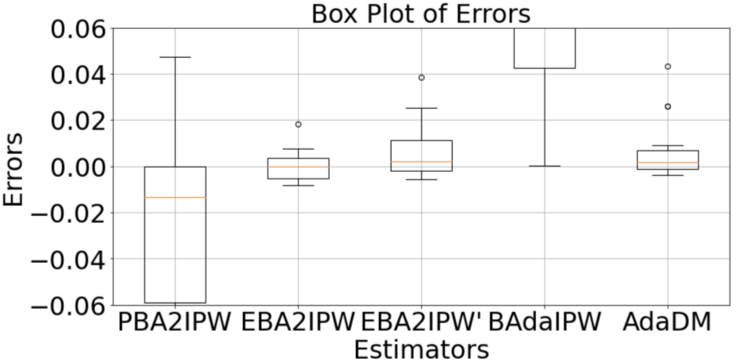
We apply our estimators to evaluate a policy using the real-world dataset in CyberAgent Inc., which is the second-largest Japanese advertisement company with about billion USD market capitalization (as of August 2020). This company simultaneously runs Thompson sampling and uniformly random sampling to determine the design of advertisements. The Thompson sampling updates the parameter every minute; therefore, there are batches with samples obtained during the minute. We use the logged data produced by the algorithms to confirm the empirical performance of the proposed estimators. To check the performance, we calculate the estimation error between the estimates of the value of the uniformly random sampling policy estimated from the dataset obtained by the Thompson sampling and the observed average reward of the uniformly random policy. More details are shown in Appendix G.2. We apply the PBA2IPW, EBA2IPW, EBA2IPW’, BAdaIPW, and AdaDM estimators. The results are shown in Table 5 and Figure 1. We show the Bias, MSE, and averaged confidence intervals. While the PBA2IPW and BAdaIPW estimators suffer the high variance, the EBA2IPW, EBA2IPW’, and AdaDM estimators show the preferable performances. Although the AdaDM estimator also shows the effectiveness for this dataset, the BA2IPW estimator is theoretically more robust because it is consistent even if does not converge to .
| Bias | MSE | ||
|---|---|---|---|
| PBA2IPW | -0.01766 | 8.25830e-02 | 8.25830e-02 |
| EBA2IPW | 0.00019 | 4.52574e-05 | 3.58261e-03 |
| EBA2IPW’ | 0.00095 | 4.03248e-05 | 2.92494e-03 |
| BAdaIPW | 0.14650 | 5.70524e-02 | 7.68610e-02 |
| AdaDM | 0.00714 | 2.26107e-04 | 2.23604e-05 |
8 Conclusion
This study presented solutions for causal inference from dependent samples obtained via a batch-based bandit algorithm. By using the asymptotic property in batch, we applied the CLT for an MDS to obtain the asymptotic normality without requiring the convergence of the assignment probability. Additionally, we showed that the proposed method is applicable when the support of arms is incomplete, which is a notorious problem in OPE. In experiments, the proposed batch-based estimators showed theoretically expected performances for benchmark and real-world datasets.
References
- Beygelzimer & Langford (2009) Beygelzimer, A. and Langford, J. The offset tree for learning with partial labels. In KDD, 2009.
- Bibaut et al. (2019) Bibaut, A., Malenica, I., Vlassis, N., and Van Der Laan, M. More efficient off-policy evaluation through regularized targeted learning. In ICML, 2019.
- Bickel et al. (1998) Bickel, P. J., Klaassen, C. A. J., Ritov, Y., and Wellner, J. A. Efficient and Adaptive Estimation for Semiparametric Models. Springer, 1998.
- Chernozhukov et al. (2018) Chernozhukov, V., Chetverikov, D., Demirer, M., Duflo, E., Hansen, C., Newey, W., and Robins, J. Double/debiased machine learning for treatment and structural parameters. Econometrics Journal, 21:C1–C68, 2018.
- Chu et al. (2011) Chu, W., Li, L., Reyzin, L., and Schapire, R. Contextual bandits with linear payoff functions. In AISTATS, 2011.
- Dudík et al. (2011) Dudík, M., Langford, J., and Li, L. Doubly Robust Policy Evaluation and Learning. In ICML, 2011.
- Farajtabar et al. (2018) Farajtabar, M., Chow, Y., and Ghavamzadeh, M. More robust doubly robust off-policy evaluation. ICML, 2018.
- Greene (2003) Greene, W. Econometric Analysis. Pearson Education, 2003.
- Hadad et al. (2019) Hadad, V., Hirshberg, D. A., Zhan, R., Wager, S., and Athey, S. Confidence intervals for policy evaluation in adaptive experiments. arXiv:1911.02768, 2019.
- Hahn (1998) Hahn, J. On the role of the propensity score in efficient semiparametric estimation of average treatment effects. Econometrica, 66:315–331, 1998.
- Hahn et al. (2011) Hahn, J., Hirano, K., and Karlan, D. Adaptive experimental design using the propensity score. Journal of Business and Economic Statistics, 29(1):96–108, 2011.
- Hall et al. (2014) Hall, P., Heyde, C., Birnbaum, Z., and Lukacs, E. Martingale Limit Theory and Its Application. Communication and Behavior. Elsevier Science, 2014.
- Hamilton (1994) Hamilton, J. Time series analysis. Princeton Univ. Press, 1994.
- Hirano et al. (2003) Hirano, K., Imbens, G. W., and Ridder, G. Efficient estimation of average treatment effects using the estimated propensity score. Econometrica, 71(4):1161–1189, 2003.
- Kallus & Uehara (2019) Kallus, N. and Uehara, M. Intrinsically efficient, stable, and bounded off-policy evaluation for reinforcement learning. arXiv:1906.03735, 2019.
- Kato et al. (2020a) Kato, M., Ishihara, T., Honda, J., and Narita, Y. Adaptive experimental design for efficient treatment effect estimation: Randomized allocation via contextual bandit algorithm. arXiv:2002.05308, 2020a.
- Kato et al. (2020b) Kato, M., Uehara, M., and Yasui, S. Off-policy evaluation and learning for external validity under a covariate shift. arXiv:2002.11642, 2020b.
- Klaassen (1987) Klaassen, C. A. J. Consistent estimation of the influence function of locally asymptotically linear estimators. Ann. Statist., 1987.
- Li et al. (2010) Li, L., Chu, W., Langford, J., and Schapire, R. E. A contextual-bandit approach to personalized news article recommendation. In WWW, 2010.
- Loeve (1977) Loeve, M. Probability Theory. Graduate Texts in Mathematics. Springer, 1977.
- Luedtke & van der Laan (2016) Luedtke, A. R. and van der Laan, M. J. Statistical inference for the mean outcome under a possibly non-unique optimal treatment strategy. Annals of statistics, 2016.
- Narita et al. (2019) Narita, Y., Yasui, S., and Yata, K. Efficient counterfactual learning from bandit feedback. In AAAI, volume 33, 2019.
- Oberst & Sontag (2019) Oberst, M. and Sontag, D. Counterfactual off-policy evaluation with gumbel-max structural causal models. In ICML, volume 97, pp. 4881–4890, 2019.
- Perchet et al. (2016) Perchet, V., Rigollet, P., Chassang, S., and Snowberg, E. Batched bandit problems. Ann. Statist., 44(2):660–681, 04 2016.
- Robins et al. (1994) Robins, J. M., Rotnitzky, A., and Zhao, L. P. Estimation of regression coefficients when some regressors are not always observed. Journal of the American Statistical Association, 89:846–866, 1994.
- Rubin (1987) Rubin, D. B. Multiple Imputation for Nonresponse in Surveys. Wiley, New York, 1987.
- Sachdeva et al. (2020) Sachdeva, N., Su, Y., and Joachims, T. Off-policy bandits with deficient support. In KDD, 2020.
- Sutton & Barto (1998) Sutton, R. S. and Barto, A. G. Reinforcement Learning: An Introduction. MIT Press, 1998.
- Swaminathan & Joachims (2015) Swaminathan, A. and Joachims, T. Batch learning from logged bandit feedback through counterfactual risk minimization. JMLR, 16:1731–1755, 2015.
- van der Laan (2008) van der Laan, M. J. The construction and analysis of adaptive group sequential designs. U.C. Berkeley Division of Biostatistics Working Paper Series, 2008.
- van der Laan & Lendle (2014) van der Laan, M. J. and Lendle, S. D. Online targeted learning. 2014.
- van der Vaart (1998) van der Vaart, A. W. Asymptotic statistics. Cambridge University Press, Cambridge, UK, 1998.
- Wang et al. (2017) Wang, Y.-X., Agarwal, A., and Dudik, M. Optimal and adaptive off-policy evaluation in contextual bandits. In ICML, 2017.
- Yang & Zhu (2002) Yang, Y. and Zhu, D. Randomized allocation with nonparametric estimation for a multi-armed bandit problem with covariates. Annals of statistics, 30(1):100–121, 02 2002.
- Zhang et al. (2020) Zhang, K. W., Janson, L., and Murphy, S. A. Inference for batched bandits. arXiv:2002.032172, 2020.
- Zheng & van der Laan (2011) Zheng, W. and van der Laan, M. J. Cross-validated targeted minimum-loss-based estimation. In Targeted Learning: Causal Inference for Observational and Experimental Data, Springer Series in Statistics. 2011.
Appendix A Preliminaries
A.1 Mathematical Tools
Proposition 1.
[Slutsky Theorem, Greene 2003, Theorem D. 16 1, p. 1117] If and , then
Definition 1.
[Uniformly Integrable, Hamilton 1994, p. 191] A sequence is said to be uniformly integrable if for every there exists a number such that
for all .
Proposition 2.
[Sufficient Conditions for Uniformly Integrable, Hamilton 1994, Proposition 7.7, p. 191] (a) Suppose there exist and such that for all . Then is uniformly integrable. (b) Suppose there exist and such that for all . If with , then is uniformly integrable.
Proposition 3 ( Convergence Theorem, Loeve 1977).
Let , suppose that for all and that as . The following are equivalent:
-
(i) in as ;
-
(ii) as ;
-
(iii) is uniformly integrable.
A.2 Martingale Limit Theorems
Proposition 4.
[Weak Law of Large Numbers for Martingale, Hall et al. 2014] Let be a martingale and a sequence of positive constants with as . Then, writing , , we have that as if
- (i)
-
;
- (ii)
-
, and;
- (iii)
-
.
Remark 5.
The weak law of large numbers for martingale holds when the random variable is bounded by a constant.
Proposition 5.
[Central Limit Theorem for a Martingale Difference Sequence, Hamilton 1994, Proposition 7.9, p. 194] Let be an -dimensional vector martingale difference sequence with . Suppose that (a) , a positive definite matrix with , a positive definite matrix; (b) for all and all , and (including ), where is the -th element of vector ; and (c) . Then .
Appendix B Generalized Method of Martingale Difference Moments
In this section, using martingale difference sequences, we establish a frameworks of GMM with samples with dependency. Let be a sample with the domain , be the space of a parameter , and be the number of moment conditions. For a vector-valued function and a parameter , let be a martingale difference sequence, i.e.,
| (3) |
Then, let be the moment condition defined as . For the parameter , the moment condition is zero from (3), i.e.,
Using samples , we approximate the moment condition by . Then, we define a GMM-like estimator as follows:
where is a positive definite weight matrix constructed from samples. Compared with the standard GMM, we do not assume that the samples are not i.i.d. However, from the assumption that is a martingale difference sequence, we can derive the following results on the consistency and asymptotic normality of under appropriate regularity conditions. We refer this method as Generalized Method of Martingale Difference Moments (GMMDM).
For brevity, let us denote as . Using the sequence , we define an estimator of OPE as
where . Note that we can consider that the estimator defined in (2) is an application of GMMDM with the moment condition
For the minimization problem defined in (2), we can analytically calculate the minimizer as
where is an -dimensional vector such that and is
Appendix C Proof of Theorem 4
Instead of , from the original formulation Eq. (2), we consider an estimator , where is a -dimensional positive-definite matrix. Let us note that . We prove the following theorem, which is a generalized statement of Theorem C.
Theorem 4 (Asymptotic Distribution the BA2IPW Estimator).
Proof.
For
where
we show that
where is a diagonal matrix such that the -element is
Then, from Slutsky Theorem (Proposition 1 in Appendix), we can show that
Step 1: Condition (a)
From
the matrix becomes a diagonal matrix such that the -element is
For and such that ,
Because , there exists a constant such that
Then, there exist constants such that
Here, from the assumption that for , and is bounded for , we can use convergence theorem (Proposition 3 in Appendix A). First, to use convergence theorem, we use boundedness of and Proposition 2 to derive the uniform integrability of for . Then, from convergence theorem, we have as . Using this results, we can show that, as (this also means ),
Therefore, as (),
Then, by using , , and ,
In addition, the variance does not depend on . We represent the independence by omitting the subscript , i.e.,
Therefore, we have
Thus, the matrix converges to a diagonal matrix as , where the -element of is
Step 2: Condition (b)
Because we assume that all variables are bounded, this condition holds.
Step 3: Condition (c)
Here, we check that . The -element of the matrix is
The part
converges in probability to because . The term
converges in probability to
from the weak law of large numbers for i.i.d. samples as because the samples are i.i.d. between and . ∎
Appendix D Necessity of Martingale Difference Sequences
In the proposed method, we construct a moment condition using martingale difference sequences. On the other hand, for some readers, using martingale difference sequences may look unnecessary because samples are i.i.d in each block between and . Therefore, such readers also might feel that we can use , which is an estimator of using samples until -th period, without going through constructing several estimators . However, in that case, it is difficult to guarantee the asymptotic normality of the proposed estimator. For example, we can consider Cramér-Wold theorem, which is stated as follows.
Proposition 6.
Let and be -dimensional random vectors. Then, for all ,
Let be
where is an estimator of using samples until -th period, i.e., all samples. Then, we consider the asymptotic property of . From Cramér-Wold theorem, there exists a random vector such that if and only if . Here, for , we can calculate as
Because of the existence of , the samples in the sum of the above equation have correlation each other. Therefore, in general, it is difficult to derive the asymptotic distribution of . As far as we know, it is not guaranteed that there exists the asymptotic distribution of , and it is an open problem. If there does not exist the asymptotic distribution of , we also cannot derive the asymptotic distribution of .
More intuitively, even thought random variables and follow normal distribution and they are uncorrelated, it does not guarantee follows normal distribution when they are dependent.
Appendix E BA2IPW with Incomplete Support of Actions
As an application of BA2IPW, we consider an OPE without Assumption 1, which assumes that there exists such that . In stead of Assumption 1, we consider a situation in which we are allowed to change the support of actions in each batch. For example, in the first batch, we choose an action from a set with probability larger than , but we choose an action from a set with probability larger than in the second batch. In this case, the probability of an action is in the first batch while the probability of an action is in the second batch. We often face such a kind of situation in practice. For dealing with this situation, instead of Assumption 1, we put Assumption 3. Under this assumption, if for at least one batch, we are allowed to use for .
For ease of discussion, we assume Assumption 1 for defining an estimator. The following estimator is a generalization of a BA2IPW estimator. Then, we explain the estimator still works only with Assumption 3 instead of Assumption 1. We call the estimator BA2IPW with Incomplete Support (BA2IPWIS). First, let us define
Then, let us define
As well as Theorem 4, we have
where is the variance covariance matrix of
Then, for , let us define the estimator as
where is a data-dependent -dimensional vector such that . As well as Theorem 4, we have the following corollary.
Corollary 1.
Under the same assumptions of Theorem 4,
Proof.
From the constraint of , we have
Then,
∎
Next, we consider an efficient weight that minimizes . The efficient weight can be defined as the solution of the following constraint optimization problem:
Appendix F Proof of Theorem 3
Proof.
Because the BADR estimator can be decomposed as
The last term is a special case of the BA2IPW estimator and has the asymptotic normality if , and , and Assumptions 1 and 2 hold. Then, we want to show that
Because the is fixed, we only have to consider
Here, for
we have
In the following parts, we separately show that
| (4) | ||||
and
| (5) | ||||
F.1 Proof of (4)
For any , to show that
we show that the mean is and the variance of the component converges to . Then, from the Chebyshev’s inequality, this result yields the statement.
The mean is calculated as
Because the mean is , the variance is calculated as
Then, we can decompose the variance as
For , we can vanish the covariance terms as
where . Therefore, the variance is calculated as
Then, by considering the conditional expectation,
Then, we want to show
Here, we can use
| (6) |
and
| (7) |
The first equation (F.1) is proved by
where is a constant. Here, we have used a parallelogram law from the second line to the third line. We have use , and and convergence rate conditions, from the third line to the fourth line. The second equation (F.1) is proved by Jensen’s inequality.
Besides, we can also use
| (8) |
This is proved by
where is a constant. Here, we used Hölder’s inequality and
Therefore, from the convergence theorem (Proposition 3) and the boundedness of the random variables, we can show that as ,
Therefore, for any , there exists a constant such that
Thus, the variance also converges to . Then, from Chebyshev’s inequality,
F.2 Proof of (5)
∎
Appendix G Experiments
G.1 Additional Experimental Results
In this section, we show the additional experimental results using different sample sizes, nonparametric estimator, and the numbers of batches.
In Table 6, we show the results of OPE with samples under batches using nonparametric NW regression. The upper graph shows the results with the RW policy. The lower graph shows the results with the UCB policy.
In Table 7, we show the results of OPE with samples under batches using nonparametric NW regression. The upper graph shows the results with the RW policy. The lower graph shows the results with the UCB policy.
In Table 8, we show the results of OPE with samples under batches using k-nearest neighbor (k-NN) regression. The upper graph shows the results with the RW policy. The lower graph shows the results with the UCB policy.
In Table 9, we show the results of OPE with samples under batches using nonparametric NW regression. The upper graph shows the results with the RW policy. The lower graph shows the results with the UCB policy.
In Table 10, we show the results of OPE with samples under batches using nonparametric NW regression. The upper graph shows the results with the RW policy. The lower graph shows the results with the UCB policy.
In Table 11, we show the results of OPL with samples under the UCB policy.
The best two methods are highlighted in bold.
G.2 Details of Experiments with CyberAgent Dataset
We use a logged dataset of advertisement selection. In the Cyberagent, the Thompson sampling and random sampling are simultaneously used as the behavior policies for selecting a video advertisement. An advertisement is selected as follows. First, after receiving a bid request for a user with the covariate in an online advertisement auction, we choose an advertisement campaign, which contains several video advertisements. Then, we choose a behavior policy from Thompson sampling and random sampling. At each period, the Thomson sampling is chosen with probability; otherwise, the random sampling is chosen. Following the chosen behavior policy, we select a video advertisement () from the candidates to maximize the click rate, . The Thomson sampling is updated for every minute. Each batch consists of about samples.
For the experiment, we create a new dataset from the original dataset. By combining some batches, we make datasets with samples and about batches in each dataset. We apply the OPE estimators to the dataset generated from the Thompson sampling and estimate the policy value of the random sampling. We regard the observed result of random sampling as the true policy value. The estimation error between the estimated policy value and the observed (true) policy value is reported.
| Datasets | satimage | pendigits | mnist | letter | sensorless | connect-4 | ||||||
|---|---|---|---|---|---|---|---|---|---|---|---|---|
| Metrics | MSE | SD | MSE | SD | MSE | SD | MSE | SD | MSE | SD | MSE | SD |
| PBA2IPW | 0.062 | 0.006 | 0.209 | 0.196 | 0.128 | 0.035 | 0.265 | 0.197 | 0.114 | 0.018 | 0.035 | 0.035 |
| EBA2IPW | 0.065 | 0.008 | 0.232 | 0.045 | 0.244 | 0.041 | 0.399 | 0.056 | 0.208 | 0.038 | 0.035 | 0.030 |
| EBA2IPW’ | 0.065 | 0.008 | 0.212 | 0.039 | 0.131 | 0.022 | 0.386 | 0.059 | 0.201 | 0.034 | 0.034 | 0.032 |
| BAdaIPW | 0.161 | 0.138 | 0.277 | 0.278 | 0.180 | 0.105 | 0.284 | 0.221 | 0.135 | 0.028 | 0.046 | 0.046 |
| AdaDM | 0.163 | 0.017 | 0.500 | 0.046 | 0.496 | 0.045 | 0.438 | 0.027 | 0.380 | 0.032 | 0.145 | 0.030 |
| AIPW | 0.046 | 0.005 | 0.155 | 0.069 | 0.293 | 0.034 | 0.214 | 0.118 | 0.104 | 0.014 | 0.057 | 0.036 |
| DM | 0.101 | 0.008 | 0.450 | 0.038 | 0.339 | 0.031 | 0.421 | 0.026 | 0.357 | 0.029 | 0.090 | 0.024 |
| Datasets | satimage | pendigits | mnist | letter | sensorless | connect-4 | ||||||
|---|---|---|---|---|---|---|---|---|---|---|---|---|
| Metrics | MSE | SD | MSE | SD | MSE | SD | MSE | SD | MSE | SD | MSE | SD |
| PBA2IPW | 0.070 | 0.015 | 0.125 | 0.042 | 0.160 | 0.039 | 0.331 | 0.287 | 0.257 | 0.467 | 0.053 | 0.053 |
| EBA2IPW | 0.020 | 0.001 | 0.058 | 0.006 | 0.320 | 0.061 | 0.426 | 0.028 | 0.268 | 0.055 | 0.035 | 0.031 |
| EBA2IPW’ | 0.050 | 0.005 | 0.146 | 0.033 | 0.152 | 0.023 | 0.414 | 0.025 | 0.237 | 0.038 | 0.050 | 0.048 |
| BAdaIPW | 0.108 | 0.036 | 0.176 | 0.071 | 0.237 | 0.079 | 0.372 | 0.454 | 0.304 | 0.667 | 0.081 | 0.080 |
| AdaDM | 0.089 | 0.004 | 0.275 | 0.013 | 0.442 | 0.027 | 0.431 | 0.022 | 0.319 | 0.025 | 0.099 | 0.033 |
| AIPW | 0.034 | 0.002 | 0.056 | 0.005 | 0.206 | 0.011 | 0.275 | 0.196 | 0.246 | 0.447 | 0.026 | 0.023 |
| DM | 0.012 | 0.000 | 0.070 | 0.002 | 0.231 | 0.012 | 0.375 | 0.024 | 0.211 | 0.018 | 0.018 | 0.018 |
| Datasets | satimage | pendigits | mnist | letter | sensorless | connect-4 | ||||||
|---|---|---|---|---|---|---|---|---|---|---|---|---|
| Metrics | MSE | SD | MSE | SD | MSE | SD | MSE | SD | MSE | SD | MSE | SD |
| PBA2IPW | 0.038 | 0.002 | 0.147 | 0.066 | 0.114 | 0.038 | 0.269 | 0.218 | 0.106 | 0.026 | 0.019 | 0.019 |
| EBA2IPW | 0.050 | 0.006 | 0.173 | 0.023 | 0.154 | 0.019 | 0.358 | 0.058 | 0.172 | 0.021 | 0.022 | 0.021 |
| EBA2IPW’ | 0.046 | 0.006 | 0.162 | 0.021 | 0.105 | 0.029 | 0.346 | 0.059 | 0.167 | 0.021 | 0.025 | 0.025 |
| BAdaIPW | 0.071 | 0.007 | 0.194 | 0.118 | 0.164 | 0.101 | 0.277 | 0.220 | 0.131 | 0.043 | 0.029 | 0.029 |
| AdaDM | 0.144 | 0.012 | 0.488 | 0.034 | 0.385 | 0.030 | 0.496 | 0.022 | 0.444 | 0.026 | 0.138 | 0.022 |
| AIPW | 0.032 | 0.002 | 0.117 | 0.026 | 0.203 | 0.015 | 0.207 | 0.078 | 0.101 | 0.022 | 0.054 | 0.014 |
| DM | 0.103 | 0.007 | 0.455 | 0.026 | 0.235 | 0.019 | 0.482 | 0.022 | 0.426 | 0.019 | 0.085 | 0.013 |
| Datasets | satimage | pendigits | mnist | letter | sensorless | connect-4 | ||||||
|---|---|---|---|---|---|---|---|---|---|---|---|---|
| Metrics | MSE | SD | MSE | SD | MSE | SD | MSE | SD | MSE | SD | MSE | SD |
| PBA2IPW | 0.045 | 0.003 | 0.073 | 0.011 | 0.145 | 0.099 | 0.282 | 0.236 | 0.120 | 0.047 | 0.038 | 0.038 |
| EBA2IPW | 0.013 | 0.000 | 0.030 | 0.003 | 0.143 | 0.016 | 0.435 | 0.051 | 0.192 | 0.042 | 0.024 | 0.019 |
| EBA2IPW’ | 0.023 | 0.001 | 0.055 | 0.009 | 0.091 | 0.010 | 0.404 | 0.049 | 0.159 | 0.023 | 0.027 | 0.024 |
| BAdaIPW | 0.067 | 0.008 | 0.106 | 0.030 | 0.199 | 0.105 | 0.299 | 0.249 | 0.111 | 0.020 | 0.069 | 0.069 |
| AdaDM | 0.071 | 0.002 | 0.206 | 0.006 | 0.322 | 0.013 | 0.458 | 0.020 | 0.334 | 0.019 | 0.070 | 0.018 |
| AIPW | 0.029 | 0.001 | 0.038 | 0.003 | 0.088 | 0.004 | 0.203 | 0.084 | 0.112 | 0.049 | 0.020 | 0.012 |
| DM | 0.007 | 0.000 | 0.039 | 0.001 | 0.109 | 0.005 | 0.356 | 0.021 | 0.216 | 0.013 | 0.017 | 0.008 |
| Datasets | satimage | pendigits | mnist | letter | sensorless | connect-4 | ||||||
|---|---|---|---|---|---|---|---|---|---|---|---|---|
| Metrics | MSE | SD | MSE | SD | MSE | SD | MSE | SD | MSE | SD | MSE | SD |
| PBA2IPW | 0.073 | 0.024 | 0.150 | 0.075 | 0.165 | 0.074 | 0.205 | 0.079 | 0.120 | 0.057 | 0.028 | 0.028 |
| EBA2IPW | 0.056 | 0.007 | 0.151 | 0.021 | 0.219 | 0.041 | 0.354 | 0.049 | 0.155 | 0.020 | 0.030 | 0.027 |
| EBA2IPW’ | 0.061 | 0.009 | 0.181 | 0.128 | 0.202 | 0.035 | 0.341 | 0.050 | 0.146 | 0.020 | 0.028 | 0.025 |
| BAdaIPW | 0.099 | 0.041 | 0.197 | 0.127 | 0.196 | 0.092 | 0.215 | 0.084 | 0.152 | 0.079 | 0.037 | 0.036 |
| AdaDM | 0.117 | 0.013 | 0.327 | 0.033 | 0.540 | 0.039 | 0.441 | 0.024 | 0.303 | 0.025 | 0.135 | 0.025 |
| AIPW | 0.048 | 0.008 | 0.108 | 0.035 | 0.133 | 0.021 | 0.182 | 0.046 | 0.106 | 0.030 | 0.021 | 0.021 |
| DM | 0.057 | 0.007 | 0.198 | 0.020 | 0.456 | 0.035 | 0.415 | 0.023 | 0.238 | 0.020 | 0.123 | 0.015 |
| Datasets | satimage | pendigits | mnist | letter | sensorless | connect-4 | ||||||
|---|---|---|---|---|---|---|---|---|---|---|---|---|
| Metrics | MSE | SD | MSE | SD | MSE | SD | MSE | SD | MSE | SD | MSE | SD |
| PBA2IPW | 0.058 | 0.007 | 0.116 | 0.038 | 0.149 | 0.057 | 0.208 | 0.064 | 0.119 | 0.049 | 0.041 | 0.041 |
| EBA2IPW | 0.014 | 0.000 | 0.021 | 0.001 | 0.322 | 0.104 | 0.400 | 0.040 | 0.168 | 0.047 | 0.030 | 0.022 |
| EBA2IPW’ | 0.043 | 0.007 | 0.113 | 0.043 | 0.309 | 0.072 | 0.380 | 0.038 | 0.133 | 0.022 | 0.036 | 0.024 |
| BAdaIPW | 0.082 | 0.011 | 0.140 | 0.048 | 0.197 | 0.055 | 0.255 | 0.161 | 0.164 | 0.109 | 0.058 | 0.058 |
| AdaDM | 0.056 | 0.002 | 0.108 | 0.004 | 0.454 | 0.019 | 0.409 | 0.023 | 0.205 | 0.015 | 0.070 | 0.024 |
| AIPW | 0.038 | 0.004 | 0.049 | 0.011 | 0.126 | 0.077 | 0.168 | 0.049 | 0.065 | 0.005 | 0.038 | 0.037 |
| DM | 0.013 | 0.000 | 0.048 | 0.001 | 0.264 | 0.009 | 0.301 | 0.023 | 0.060 | 0.004 | 0.011 | 0.011 |
| Datasets | satimage | pendigits | mnist | letter | sensorless | connect-4 | ||||||
|---|---|---|---|---|---|---|---|---|---|---|---|---|
| Metrics | MSE | SD | MSE | SD | MSE | SD | MSE | SD | MSE | SD | MSE | SD |
| PBA2IPW | 0.046 | 0.005 | 0.127 | 0.059 | 0.138 | 0.064 | 0.243 | 0.184 | 0.141 | 0.083 | 0.022 | 0.022 |
| EBA2IPW | 0.049 | 0.006 | 0.123 | 0.018 | 0.140 | 0.023 | 0.241 | 0.055 | 0.122 | 0.018 | 0.023 | 0.022 |
| EBA2IPW’ | 0.048 | 0.005 | 0.117 | 0.017 | 0.113 | 0.019 | 0.233 | 0.055 | 0.136 | 0.047 | 0.023 | 0.022 |
| BAdaIPW | 0.081 | 0.011 | 0.171 | 0.088 | 0.154 | 0.066 | 0.244 | 0.182 | 0.161 | 0.090 | 0.034 | 0.034 |
| AdaDM | 0.138 | 0.015 | 0.496 | 0.040 | 0.439 | 0.044 | 0.479 | 0.021 | 0.413 | 0.030 | 0.143 | 0.026 |
| AIPW | 0.034 | 0.003 | 0.100 | 0.016 | 0.249 | 0.026 | 0.172 | 0.038 | 0.107 | 0.050 | 0.061 | 0.023 |
| DM | 0.098 | 0.007 | 0.460 | 0.032 | 0.289 | 0.030 | 0.465 | 0.022 | 0.397 | 0.025 | 0.090 | 0.019 |
| Datasets | satimage | pendigits | mnist | letter | sensorless | connect-4 | ||||||
|---|---|---|---|---|---|---|---|---|---|---|---|---|
| Metrics | MSE | SD | MSE | SD | MSE | SD | MSE | SD | MSE | SD | MSE | SD |
| PBA2IPW | 0.061 | 0.007 | 0.143 | 0.082 | 0.133 | 0.045 | 0.276 | 0.222 | 0.154 | 0.065 | 0.073 | 0.073 |
| EBA2IPW | 0.023 | 0.001 | 0.068 | 0.021 | 0.168 | 0.034 | 0.401 | 0.079 | 0.185 | 0.048 | 0.028 | 0.028 |
| EBA2IPW’ | 0.047 | 0.011 | 0.080 | 0.022 | 0.117 | 0.015 | 0.384 | 0.072 | 0.171 | 0.036 | 0.032 | 0.031 |
| BAdaIPW | 0.081 | 0.018 | 0.198 | 0.129 | 0.199 | 0.082 | 0.290 | 0.258 | 0.149 | 0.042 | 0.101 | 0.100 |
| AdaDM | 0.108 | 0.006 | 0.286 | 0.012 | 0.409 | 0.021 | 0.464 | 0.019 | 0.357 | 0.026 | 0.100 | 0.030 |
| AIPW | 0.037 | 0.004 | 0.060 | 0.009 | 0.155 | 0.008 | 0.229 | 0.140 | 0.127 | 0.052 | 0.017 | 0.017 |
| DM | 0.012 | 0.000 | 0.071 | 0.001 | 0.178 | 0.009 | 0.385 | 0.022 | 0.244 | 0.018 | 0.012 | 0.012 |
| Datasets | satimage | pendigits | mnist | letter | sensorless | connect-4 | ||||||
|---|---|---|---|---|---|---|---|---|---|---|---|---|
| Metrics | MSE | SD | MSE | SD | MSE | SD | MSE | SD | MSE | SD | MSE | SD |
| PBA2IPW | 0.045 | 0.004 | 0.139 | 0.065 | 0.163 | 0.077 | 0.376 | 0.328 | 0.162 | 0.076 | 0.058 | 0.058 |
| EBA2IPW | 0.051 | 0.005 | 0.274 | 0.035 | 0.248 | 0.029 | 0.467 | 0.044 | 0.265 | 0.044 | 0.032 | 0.024 |
| EBA2IPW’ | 0.051 | 0.006 | 0.267 | 0.035 | 0.162 | 0.077 | 0.460 | 0.041 | 0.258 | 0.037 | 0.032 | 0.031 |
| BAdaIPW | 0.089 | 0.013 | 0.193 | 0.089 | 0.213 | 0.103 | 0.399 | 0.396 | 0.188 | 0.100 | 0.076 | 0.075 |
| AdaDM | 0.144 | 0.012 | 0.492 | 0.033 | 0.434 | 0.037 | 0.476 | 0.022 | 0.412 | 0.027 | 0.139 | 0.023 |
| AIPW | 0.057 | 0.021 | 0.109 | 0.024 | 0.234 | 0.018 | 0.282 | 0.127 | 0.150 | 0.062 | 0.073 | 0.057 |
| DM | 0.101 | 0.003 | 0.447 | 0.024 | 0.265 | 0.022 | 0.457 | 0.021 | 0.389 | 0.021 | 0.083 | 0.015 |
| Datasets | satimage | pendigits | mnist | letter | sensorless | connect-4 | ||||||
|---|---|---|---|---|---|---|---|---|---|---|---|---|
| Metrics | MSE | SD | MSE | SD | MSE | SD | MSE | SD | MSE | SD | MSE | SD |
| PBA2IPW | 0.052 | 0.006 | 0.089 | 0.019 | 0.131 | 0.053 | 0.372 | 1.023 | 0.117 | 0.057 | 0.037 | 0.037 |
| EBA2IPW | 0.013 | 0.000 | 0.021 | 0.001 | 0.223 | 0.015 | 0.446 | 0.037 | 0.194 | 0.025 | 0.030 | 0.017 |
| EBA2IPW’ | 0.035 | 0.002 | 0.099 | 0.013 | 0.140 | 0.065 | 0.428 | 0.028 | 0.206 | 0.028 | 0.035 | 0.028 |
| BAdaIPW | 0.071 | 0.011 | 0.125 | 0.033 | 0.194 | 0.091 | 0.387 | 1.065 | 0.138 | 0.071 | 0.055 | 0.055 |
| AdaDM | 0.054 | 0.002 | 0.197 | 0.006 | 0.350 | 0.016 | 0.444 | 0.023 | 0.310 | 0.025 | 0.066 | 0.021 |
| AIPW | 0.034 | 0.003 | 0.044 | 0.004 | 0.131 | 0.006 | 0.306 | 0.593 | 0.090 | 0.022 | 0.024 | 0.012 |
| DM | 0.011 | 0.000 | 0.041 | 0.001 | 0.151 | 0.007 | 0.359 | 0.023 | 0.196 | 0.016 | 0.020 | 0.010 |
| Datasets | satimage | pendigits | mnist | letter | sensorless | connect-4 | ||||||
|---|---|---|---|---|---|---|---|---|---|---|---|---|
| Metrics | RWD | SD | RWD | SD | RWD | SD | RWD | SD | RWD | SD | RWD | SD |
| PBA2IPW | 0.806 | 0.024 | 0.656 | 0.145 | 0.743 | 0.028 | 0.156 | 0.048 | 0.317 | 0.062 | 0.645 | 0.030 |
| EBA2IPW | 0.810 | 0.026 | 0.463 | 0.100 | 0.653 | 0.054 | 0.099 | 0.046 | 0.312 | 0.075 | 0.668 | 0.030 |
| BAdaIPW | 0.811 | 0.021 | 0.511 | 0.107 | 0.656 | 0.070 | 0.126 | 0.038 | 0.275 | 0.071 | 0.665 | 0.024 |
| AdaDM | 0.786 | 0.029 | 0.407 | 0.053 | 0.191 | 0.078 | 0.055 | 0.023 | 0.207 | 0.039 | 0.653 | 0.030 |
| AIPW | 0.819 | 0.015 | 0.419 | 0.099 | 0.644 | 0.101 | 0.120 | 0.040 | 0.290 | 0.057 | 0.666 | 0.028 |
| DM | 0.798 | 0.026 | 0.387 | 0.035 | 0.212 | 0.080 | 0.089 | 0.036 | 0.220 | 0.045 | 0.653 | 0.030 |