跳到论文正文
W Papers独立论文阅读器 arXiv:2010.13495 论文正文 计算阅读时间 · 0%
引用这篇论文根据当前论文元数据生成,正式投稿前建议核对。


License: arXiv.org perpetual non-exclusive license
arXiv:2010.13495v3 [gr-qc] 24 Dec 2020

Mimetic Inflation

Seyed Ali Hosseini Mansoori a Note: shosseini@shahroodut.ac.ir    Alireza Talebian b Note: talebian@ipm.ir    Hassan Firouzjahi b Note: firouz@ipm.ir
Abstract

We study inflationary solution in an extension of mimetic gravity with the higher derivative interactions coupled to gravity. Because of the higher derivative interactions the setup is free from the ghost and gradient instabilities while it hosts a number of novel properties. The dispersion relation of scalar perturbations develop quartic momentum correction similar to the setup of ghost inflation. Furthermore, the tilt of tensor perturbations can take either signs with a modified consistency relation between the tilt and the amplitude of tensor perturbations. Despite the presence of higher derivative interactions coupled to gravity the tensor perturbations propagate with the speed equal to the speed of light as required by the LIGO observations. Furthermore, the higher derivative interactions induce non-trivial interactions in cubic Hamiltonian, generating non-Gaussianities in various shapes such as the equilateral, orthogonal and squeezed configurations with observable amplitudes.

1 Introduction

Mimetic gravity is a novel scalar-tensor theory proposed by Chamseddine and Mukhanov Chamseddine:2013kea as a modification of General Relativity (GR). The idea is to express the physical metric gμ​νg_{\mu\nu} in the Einstein-Hilbert action by performing a conformal transformation gμ​ν=−(g~α​β​∂αϕ​∂βϕ)​g~μ​νg_{\mu\nu}=-(\tilde{g}^{\alpha\beta}\partial_{\alpha}\phi\partial_{\beta}\phi)\tilde{g}_{\mu\nu} from an auxiliary metric g~μ​ν\tilde{g}_{\mu\nu} in which ϕ\phi is a scalar field. As a result, the longitudinal mode of gravity becomes dynamical even in the absence of any matter source. The above transformation can also be considered as a singular limit of the general disformal transformation where the transformation is not invertible Deruelle:2014zza; Yuan:2015tta. With the physical metric, the scalar field is subject to the constraint11 1 We use the mostly positive signature for the metric.,

gμ​ν​∂μϕ​∂νϕ=−1.g^{\mu\nu}\partial_{\mu}\phi\partial_{\nu}\phi=-1. (1)

As a consequence of this constraint, the theory mimics the roles of cold dark matter in cosmic expansion, hence the theory is dubbed as the mimetic dark matter. The original mimetic model was then extended to inflation, dark energy and also theories with non-singular cosmological and black hole solutions Chamseddine:2014vna; Chamseddine:2016uef; Chamseddine:2016ktu. See also Refs. Mirzagholi:2014ifa; Myrzakulov:2015kda; Arroja:2015yvd; Sebastiani:2016ras; Dutta:2017fjw; Saadi:2014jfa; Firouzjahi:2018xob; Gorji:2019rlm; Matsumoto:2015wja; Momeni:2015aea; Astashenok:2015qzw; Sadeghnezhad:2017hmr; Nozari:2019esz; Solomon:2019qgf; Shen:2019nyp; Ganz:2019vre; deCesare:2019pqj; Nozari:2019shm; deCesare:2018cts; Ganz:2018mqi; Ganz:2018vzg; Sheykhi:2019gvk; Sheykhi:2020dkm; Sheykhi:2020fqf; Nojiri:2014zqa; Astashenok:2015haa; Nojiri:2016ppu; Nojiri:2017ygt; Nojiri:2016vhu; Odintsov:2018ggm; Casalino:2018wnc for further theoretical developments in mimetic gravity.

The original version of the mimetic theory is free from instabilities Barvinsky:2013mea; Chaichian:2014qba, but there is no nontrivial dynamics for scalar-type fluctuations. In order to circumvent this problem, the higher derivative term (□​ϕ)2(\Box\phi)^{2} is added to the original action which generates a dynamical scalar degree of freedom propagating with a nonzero sound speed Chamseddine:2014vna; Mirzagholi:2014ifa. In addition, the mimetic model with a general higher derivative function in the form f⁡(□​ϕ)f(\Box\phi) has been considered in Refs. Chamseddine:2016uef; Chamseddine:2016ktu. However, these extended mimetic setups with a propagating scalar degree of freedom are plagued with the ghost and the gradient instabilities Ijjas:2016pad; Firouzjahi:2017txv; Ramazanov:2016xhp22 2 The mimetic dark matter scenario also suffers from caustics Capela:2014xta, see also DeFelice:2015moy; Gumrukcuoglu:2016jbh; Babichev:2016jzg; Babichev:2017lrx. It should be noted that the gauge field extensions of the mimetic scenario potentially avoid caustics formations Gorji:2018okn; Gorji:2019ttx.. To remedy these issues, it was suggested in Zheng:2017qfs; Hirano:2017zox; Gorji:2017cai to extend the mimetic model further by considering direct couplings of the higher derivative terms to the curvature tensor of the spacetime such as □​ϕ​R\Box\phi R, ∇μ∇ν​ϕ​Rμ​ν\nabla_{\mu}\nabla_{\nu}\phi R^{\mu\nu}, □​ϕ​∇μϕ​∇νϕ​Rμ​ν\Box\phi\nabla_{\mu}\phi\nabla_{\nu}\phi R^{\mu\nu} and so on. By appropriate choices of these higher derivative couplings one can bypass the problems of the gradient and the ghost instabilities. However, now the background dynamics is more complicated and a simple dark mater solution is not a direct outcome of the analysis.

In this work our goal is to construct inflationary solutions in the extended mimetic setup with the effects of higher derivative couplings taking into account. As we will see the presence of higher derivative couplings to gravity generate new interactions and the analysis of cosmological perturbations become non-trivial. For example, because of these higher derivative interactions the dispersion relation of scalar perturbations receive higher order corrections resembling non-relativistic dispersion relation as in ghost inflation setup ArkaniHamed:2003uz. In addition, the predictions for the tensor perturbations are modified with a new consistency condition between the scalar spectral index nsn_{s}, the sound speed of scalar perturbations csc_{s} and the tensor to scalar ratio rtr_{t}.

Because of the higher derivative interactions, the model predicts novel non-Gaussianity features. The situation here is somewhat similar to the EFT studies of higher derivative corrections to the single field model Cheung:2007st where large non-Gaussianity of various shapes such as equilateral and orthogonal types can be generated. In addition, similar to models with a non-standard kinetic energy such as DBI model Alishahiha:2004eh, the sound speed of scalar perturbations play non-trivial roles in generating large non-Gaussianities. The strong observational bounds on primordial non-Gaussianities can be used to constrain the model parameters. More specifically, the amplitude of non-Gaussianity parameter fNLf_{{}_{\rm NL}} in the squeezed, equilateral and orthogonal configurations from the Planck observations (Akrami:2018odb; Akrami:2019izv) are constrained to be

fNLsq=−0.9±5.1,fNLequi=−26±47,fNLortho=−38±24(68%CL).f_{{}_{\rm NL}}^{\rm sq}=-0.9\pm 5.1,\hskip 28.45274ptf_{{}_{\rm NL}}^{\rm equi}=-26\pm 47,\hskip 28.45274ptf_{{}_{\rm NL}}^{\rm ortho}=-38\pm 24\hskip 7.11317pt(68\%\rm CL)\,. (2)

We shall use these bounds to constrain model parameters and various couplings.

The organization of the paper is as follows. In next Section, we present our setup and construct the background solutions which mimic cold dark matter even in the absence of normal matter. Then we extend these analysis to obtain an inflationary solution. In Section 3 we obtain the power spectrum of the curvature and tensor perturbations and calculate various cosmological observables. In Section 4, we study bispectrum and calculate the non-Gaussianity parameter fNLf_{{}_{\rm NL}} for local, equilateral and orthogonal configurations numerically, followed by discussions and summaries in Section 5. Many technical analysis of cosmological perturbations associated to power spectra and scalar bispectrum are relegated to Appendices A and B.

2 Inflationary Solution

In this section we study the background dynamics to obtain a period of inflation in early universe.

As summarized in Introduction, to remedy the ghost and gradient instabilities various higher derivative terms are added to the mimetic setup. Besides the higher derivative terms such as (□​ϕ)2(\Box\phi)^{2} and ∇μ∇ν​ϕ​∇μ​∇νϕ\nabla_{\mu}\nabla_{\nu}\phi\nabla^{\mu}\nabla^{\nu}\phi, we also require the higher derivative couplings of of the mimetic field to the curvature of the spacetime such as □​ϕ​R\Box\phi R, ∇μ∇ν​ϕ​Rμ​ν\nabla_{\mu}\nabla_{\nu}\phi R^{\mu\nu}, □​ϕ​∇μϕ​∇νϕ​Rμ​ν\Box\phi\nabla_{\mu}\phi\nabla_{\nu}\phi R^{\mu\nu} and so on Zheng:2017qfs; Hirano:2017zox; Gorji:2017cai. Here we restrict ourselves to the simplest case where there is only a direct coupling of the higher derivative term □​ϕ≡χ\Box\phi\equiv\chi to the Ricci scalar as follows,

S=∫d4​x​−g​[MP22​F​(χ)​R+λ⁡(gα​β​∂αϕ​∂βϕ+1)+P⁡(χ)−V⁡(ϕ)],\displaystyle S=\int{\rm d}^{4}x\sqrt{-g}\left[\frac{{M}_{\rm P}^{2}}{2}F(\chi)R+\lambda\left(g^{\alpha\beta}\partial_{\alpha}\phi\partial_{\beta}\phi+1\right)+P(\chi)-V(\phi)\right]\,, (3)

in which MPM_{\rm P} is the reduced Planck mass 33 3 The Hamiltonian analysis of this model have also been investigated in Ref Zheng:2018cuc in both Einstein frame and Jordan frame.. The Lagrangian multiplier λ\lambda enforces the constraint Eq. (1) Golovnev:2013jxa. In addition, we have allowed a potential term for the mimetic field which will drive inflation. In this setup PP and FF are arbitrary smooth function of χ\chi. The former is added to make the scalar perturbation propagating (i.e. inducing a non-zero csc_{s} ) while the latter is required to remedy the gradient and the ghost instabilities Zheng:2017qfs; Hirano:2017zox; Gorji:2017cai. As mentioned before, more complicated function of derivatives of ϕ\phi and χ\chi such as F2​(∇μ∇ν​ϕ​Rμ​ν)F_{2}(\nabla_{\mu}\nabla_{\nu}\phi R^{\mu\nu}) and F3​(χ​∇μϕ​∇νϕ​Rμ​ν)F_{3}(\chi\nabla_{\mu}\phi\nabla_{\nu}\phi R^{\mu\nu}) can also be added along with the simple function F⁡(χ)F(\chi). However, the analysis even in the simplest setup of action (3) is complicated enough so we do not consider models with other higher derivative couplings.

Before presenting the fields equation one important comment is in order. In the action (3) the effective gravitational coupling (effective reduced Planck mass) is actually MP​F​(χ)1/2M_{\rm P}F(\chi)^{1/2}. We can perform the calculations in the given “Jordan frame” but with a proper interpretation of the physical gravitational coupling. Alternatively, we may perform a metric field redefinition and go to the “Einstein frame” where the gravitational coupling is simply MPM_{\rm P}. The latter is rather complicated as the model presented in action (3) contains various higher derivative terms. Instead, we follow the first approach and work in the original Jordan frame. However, we make a further assumption that at the end of inflation the fields ϕ\phi becomes trivial with F⁡(χe)=1F(\chi_{e})=1 and one recovers the standard GR afterwards. This is a simplification made based on the intuitive ground though we do not have a dynamical mechanism to enforce it. We leave it as an open question as how or whether this transition from a mimetic setup to a standard GR setup can be achieved at the end of inflation. With these discussions in mind, we set MP=1M_{\rm P}=1 in the rest of the analysis.

By taking the variation of the action (3) with respect to the inverse metric gμ​νg^{\mu\nu}, one obtains the Einstein field equations as F⁡(χ)​Gμ​ν=Tμ​νF(\chi)G_{\mu\nu}=T_{\mu\nu} where Gμ​νG_{\mu\nu} is the Einstein tensor and Tμ​νT_{\mu\nu} is the effective energy momentum tensor, given by

Tνμ\displaystyle T^{\mu}_{\nu} =\displaystyle= −2λ∂μϕ∂vϕ+[∂μPχ∂νϕ+∂μϕ∂νPχ+12(∂μϕ∂ν(RFχ)+∂νϕ∂μ(RFχ))+∇μ∂νF]\displaystyle-2\lambda{{\partial}^{\mu}}\phi{{\partial}_{v}}\phi+\left[{{\partial}^{\mu}}P_{\chi}{{\partial}_{\nu}}\phi+{{\partial}^{\mu}}\phi{{\partial}_{\nu}}P_{\chi}+\frac{1}{2}\Big(\partial^{\mu}\phi\partial_{\nu}(RF_{\chi})+\partial_{\nu}\phi\partial^{\mu}(RF_{\chi})\Big)+\nabla^{\mu}\partial_{\nu}F\right] (4)
+\displaystyle+ δνμ​[P−χ​Pχ−V−gα​β​∂αPχ​∂βϕ−12​∇α(R​∂αϕ​Fχ)+□​F],\displaystyle\delta_{\nu}^{\mu}\left[P-\chi P_{\chi}-V-{{g}^{\alpha\beta}}{{\partial}_{\alpha}}P_{\chi}{{\partial}_{\beta}}\phi-\frac{1}{2}\nabla^{\alpha}\Big(R\partial_{\alpha}\phi F_{\chi}\Big)+\Box F\right]\,,

in which Pχ≡∂P/∂χ{P}_{\chi}\equiv\partial{P}/\partial\chi and so on. In obtaining the above expression we have implemented the mimetic constraint (1). Clearly the energy momentum tensor given above can not be cast into the form of the energy momentum tensor of a perfect fluid.

Moreover, varying the action (3) with respect to the scalar filed ϕ\phi gives the following modified Klein-Gordon equation,

1−g​∂μ[−g​(2​λ​∂μϕ−∂μ(Pχ+12​R​Fχ))]+∂V⁡(ϕ)∂ϕ=0.\frac{1}{\sqrt{-g}}{{\partial}_{\mu}}\Big[\sqrt{-g}\Big(2\lambda{{\partial}^{\mu}}\phi-{{\partial}^{\mu}}\big(P_{\chi}+\frac{1}{2}RF_{\chi}\big)\Big)\Big]+\frac{\partial V\left(\phi\right)}{\partial\phi}=0\,. (5)

The background cosmological solution is in the form of FRLW universe with the metric

d​s2=−d​t2+a​(t)2​d​𝐱2,\displaystyle{\rm d}s^{2}=-{\rm d}t^{2}+a(t)^{2}{\rm d}{\bf{x}}^{2}\,, (6)

in which tt and aa are the cosmic time and the scale factor respectively. One can check that the background field equations take the following forms

3​F​H2\displaystyle 3FH^{2} =\displaystyle= V−2​λ−(P+3​H​Pχ+3​H˙​Pχ​χ)−3​(6​H3​Fχ−4​H​H˙​Fχ+6​H2​H˙​Fχ​χCLOSE\displaystyle V-2\lambda-\big(P+3HP_{\chi}+3\dot{H}P_{\chi\chi}\big)-3\Big(6H^{3}F_{\chi}-4H\dot{H}F_{\chi}+6H^{2}\dot{H}F_{\chi\chi} (7)
+\displaystyle+ OPEN3​H˙2​Fχ​χ−H¨​Fχ),\displaystyle 3\dot{H}^{2}F_{\chi\chi}-\ddot{H}F_{\chi}\Big)\,,

and

F⁡(2​H˙+3​H2)=V−(P+3​H​Pχ−3​H˙​Pχ​χ)−3​H​(Fχ​(6​H2+5​H˙)−6​H​H˙​Fχ​χ),\displaystyle F(2\dot{H}+3H^{2})=V-(P+3HP_{\chi}-3\dot{H}P_{\chi\chi})-3H\Big(F_{\chi}(6H^{2}+5\dot{H})-6H\dot{H}F_{\chi\chi}\Big)\,, (8)

where H=a˙​(t)/a​(t)H=\dot{a}(t)/a(t) is the Hubble expansion rate. Note that at the background level, the mimetic constraint (1) enforces ϕ˙=1\dot{\phi}=1 and correspondingly χ=−3​H\chi=-3H.

Before constructing the inflationary solution, let us for the moment set V=0V=0 to see how the mimetic setup can yield the dark matte solution. Using Eq. (5) the Lagrangian multiplier is obtained as follows

λ=𝒞2​a3+6​H​H˙​Fχ−9​H2​H˙​Fχ​χ−92​H˙2​Fχ​χ−32​H˙​Pχ​χ+32​H¨​Fχ(V=0),\lambda=\frac{\mathcal{C}}{2a^{3}}+6H\dot{H}F_{\chi}-9H^{2}\dot{H}F_{\chi\chi}-\dfrac{9}{2}\dot{H}^{2}F_{\chi\chi}-\dfrac{3}{2}\dot{H}P_{\chi\chi}+\dfrac{3}{2}\ddot{H}F_{\chi}\quad\quad(V=0)\,, (9)

in which 𝒞\mathcal{C} is an integration constant. Plugging this into the Friedmann equation (7), one obtains

3​H22​[F+6​H​Fχ+13​H2​(P+3​H​Pχ)]=−𝒞a3(V=0).\frac{3H^{2}}{2}\Big[F+6HF_{\chi}+\dfrac{1}{3H^{2}}(P+3HP_{\chi})\Big]=-\frac{\mathcal{C}}{a^{3}}\quad\quad(V=0)\,. (10)

The constant 𝒞\mathcal{C} above indicates that a dark matter type solution can exist. However, in order for this conclusion to be valid we require the combination in the big bracket in Eq. (10) to be a constant. Since this combination plays important roles in our analysis below let us define

F+6​H​Fχ+13​H2​(P+3​H​Pχ)≡−𝒦.\displaystyle F+6HF_{\chi}+\dfrac{1}{3H^{2}}(P+3HP_{\chi})\equiv-\mathcal{K}\,. (11)

Using this definition of the function 𝒦\mathcal{K} and taking the time derivative of Eq. (10) once more, we obtain

2​H˙+3​H2=−H​𝒦˙𝒦,(V=0).\displaystyle 2\dot{H}+3H^{2}=-\frac{H\dot{\mathcal{K}}}{\mathcal{K}}\,,\quad\quad(V=0)\,. (12)

For a dark matter solution with a∼t2/3a\sim t^{2/3}, the left hand side of Eq. (12) vanishes so indeed to have a dark matter solution we require the function 𝒦\mathcal{K} to be constant. In this case the Friedmann equation simplifies to 3​H2=𝒞~/a3=ρ3H^{2}=\tilde{\mathcal{C}}/a^{3}=\rho where ρ\rho is the effective energy density and 𝒞~≡2​𝒞/𝒦\tilde{\mathcal{C}}\equiv 2\mathcal{C}/\mathcal{K}. To have a consistent solution one requires that 𝒞~>0\tilde{\mathcal{C}}>0 while there is no restriction on the signs of 𝒞\mathcal{C} and 𝒦\mathcal{K} separately at this level. For example, in the original mimetic setup with F=1F=1 and P=0P=0, one obtains 𝒦=−1\mathcal{K}=-1 and the dark matter solution is a direct outcome of the analysis. In conclusion, while the functions P⁡(χ)P(\chi) and F⁡(χ)F(\chi) are arbitrary, but in order to obtain a dark matter candidate in this setup one requires the combination 𝒦\mathcal{K} defined in Eq. (11) to be a constant.

Now we consider the case when V⁡(ϕ)=V⁡(t)≠0V(\phi)=V(t)\neq 0 in order to obtain inflationary solution. Starting with the second Einstein equation (8) and using the definition of 𝒦\mathcal{K} to eliminate the combinations containing Fχ​χF_{\chi\chi} and Pχ​χP_{\chi\chi} in favours of 𝒦˙\dot{\mathcal{K}} we obtain

2​H˙+3​H2=−H​𝒦˙𝒦+V𝒦.2\dot{H}+3H^{2}=-\frac{H\dot{\mathcal{K}}}{\mathcal{K}}+\dfrac{V}{\mathcal{K}}\,. (13)

In particular, if we set V=0V=0, we recover Eq. (12) as expected. Now noting that

2​H˙+3​H2+H​𝒦˙𝒦=1a3​H2​𝒦​dd​t​(a3​H2​𝒦),\displaystyle 2\dot{H}+3H^{2}+\frac{H\dot{\mathcal{K}}}{\mathcal{K}}=\frac{1}{a^{3}H^{2}\mathcal{K}}\frac{d}{dt}\Big(a^{3}H^{2}\mathcal{K}\Big)\,, (14)

we can integrate Eq. (13) to obtain

3​H2=1𝒦​a3​(𝒞−3​∫d​a​a2​V),\displaystyle 3H^{2}=\frac{1}{\mathcal{K}\,a^{3}}\Big(\mathcal{C}-3\int{\rm d}a\,a^{2}V\Big)\,, (15)

in which as in previous case 𝒞\mathcal{C} is a constant.

In an inflationary background one can neglect the constant term 𝒞\mathcal{C} in Eq. (15) as it is diluted rapidly. In addition, if VV is nearly flat as in conventional slow-roll scenarios then we can obtain a phase of near dS spacetime with H2≃−V/𝒦H^{2}\simeq-V/\mathcal{K}. Now we see the curious effect that in order to obtain an inflationary background we require the signs of VV and 𝒦\mathcal{K} to be opposite. However, as we shall see in nest section, in order to have healthy scalar and tensor perturbations we require 𝒦>0\mathcal{K}>0. As a result, to obtain an inflationary solution in this setup we need a negative potential. This should be compared with the analysis in Chamseddine:2014vna where F=1F=1, P⁡(χ)=γ2​χ2P(\chi)=\frac{\gamma}{2}\chi^{2} and V>0V>0. For these values of FF and PP we obtain 𝒦=−1+3​γ/2\mathcal{K}=-1+3\gamma/2. On the other hand, the sound speed of scalar perturbations in the model of Chamseddine:2014vna is cs2=γ/(2−3​γ)c_{s}^{2}=\gamma/(2-3\gamma) so 𝒦\mathcal{K} has opposite sign compared to cs2c_{s}^{2} (with OPENγ>0)\gamma>0). Now in order to avoid the gradient instability one requires cs2>0c_{s}^{2}>0 so in their inflationary solution they need 𝒦<0\mathcal{K}<0. But as we shall see in next section the sign of the quadratic action for the scalar perturbations is proportional to the sign of 𝒦\mathcal{K} so a negative 𝒦\mathcal{K} indicates the propagation of ghost as pointed out in details in Firouzjahi:2017txv. As we mentioned above, this problem arises because in the analysis of Chamseddine:2014vna they considered V>0V>0 to construct inflationary solution.

Although the mimetic field ϕ\phi is not an ordinary “rolling" scalar field in the sense that it appears with a constraint in the setup, but the requirement of a negative potential looks unexpected. However, we remind that negative potentials have been employed in the past in other contexts such as in contracting universes Khoury:2001wf; Kallosh:2001ai; Finelli:2001sr; Buchbinder:2007ad; Buchbinder:2007tw, see also Linde:2001ae; Hartle:2012qb.

To construct a specific inflationary setup, we consider the inverted quadratic potential as follows

V⁡(ϕ)={−12​m2​ϕ2t<00t>0,ϕ=t\displaystyle V(\phi)=\Bigg\{\begin{array}[]{ll}-\frac{1}{2}m^{2}\phi^{2}&~~~~~~~~t<0\\ 0&~~~~~~~~t>0\\ \end{array},~~~~\hskip 14.22636pt\phi=t

Inflation occurs when t<0t<0 while the hot big bang phase follows inflation for t>0t>0. We obtain the inflationary phase as the field rolls up the negative potential toward the origin. In addition, we assume that the potential vanishes for t>0t>0, so as discussed below Eq. (12), the seeds of observed dark matter can be obtained in this setup when inflation ends.

So far our analysis were general and we did not specify the forms of the functions F⁡(χ)F(\chi) and P⁡(χ)P(\chi), unless we require the combination 𝒦\mathcal{K} to be positive. From now one, we further demand that 𝒦\mathcal{K} is a constant which simplifies the construction of the inflationary solution greatly. Now by introducing the new variable y≡a32y\equiv a^{\frac{3}{2}}, Eq. (13) becomes a linear differential equation,

y¨−3​m2​t28​𝒦​y=0,(t<0)\ddot{y}-\frac{3m^{2}t^{2}}{8\mathcal{K}}y=0\,,\quad\quad(t<0) (19)

which is similar to Eq. (31) in Ref. Chamseddine:2014vna.

The inflationary branch of the solution is given by

y⁡(t)=−t​K14​(332​𝒦​m​t2),\displaystyle y(t)=\sqrt{-t}~K_{\frac{1}{4}}\Big(\sqrt{\dfrac{3}{32\mathcal{K}}}~m\,t^{2}\Big)\,, (20)

in which Kν​(x)K_{\nu}(x) is the modified Bessel function of the second kind. At large negative tt, one finds that the scale factor grows as

a∝(−t)−13​exp⁡(−m​t22​6​𝒦),a\propto(-t)^{-\frac{1}{3}}\exp\big(-\frac{mt^{2}}{2\sqrt{6\mathcal{K}}}\big)\,, (21)

whereas it is proportional to (t)2/3(t)^{2/3} for positive tt after inflation which is the indication of a dark matter dominated universe. Of course, we have to include reheating where radiation should be generated after inflation.

The behaviours of the corresponding slow-roll parameters,

ϵH≡−H˙H2,ϵH(2)≡ϵ˙HHϵH,\displaystyle\epsilon_{{}_{H}}\equiv-\dfrac{\dot{H}}{H^{2}}\,,\hskip 28.45274pt\epsilon_{{}_{H}}^{{}_{(2)}}\equiv\dfrac{\dot{\epsilon}_{{}_{H}}}{H\,\epsilon_{{}_{H}}}\,, (22)

are shown in Fig. 1. One can easily satisfy the conditions ϵH,ϵH(2)≪1\epsilon_{{}_{H}},\ \epsilon_{{}_{H}}^{{}_{(2)}}\ll 1 to obtain 50−6050-60  number of e-folds to solve the flatness and the horizon problems. As usual, inflation ends when either of the slow-roll parameters approach order of unity. It should be noted that these slow-roll conditions are independent of the values of mm and 𝒦{\cal K}.

Figure 1: The first and second slow-roll parameters associated to the scale factor (21) in terms of the number of e-folds NN. These behaviours are independent from the values of mm and 𝒦{\cal K}.

For the future uses, let us define the slow-roll parameters associated with the background functions such as HH, FF etc as follows

ϵX(1)≡ϵX\displaystyle\epsilon_{{}_{X}}^{{}_{(1)}}\equiv\epsilon_{{}_{X}} ≡±X˙H​XandϵX(n)≡ϵ˙X(n−1)HϵX(n−1)forn≥2.\displaystyle\equiv\pm\dfrac{\dot{X}}{H\ X}\hskip 7.11317pt\text{and}\hskip 7.11317pt\epsilon_{{}_{X}}^{{}_{(n)}}\equiv\dfrac{\dot{\epsilon}_{{}_{X}}^{{}_{(n-1)}}}{H\ \epsilon_{{}_{X}}^{{}_{(n-1)}}}\hskip 7.11317pt\text{for}\hskip 7.11317ptn\geq 2\,. (23)

Note that the minus sign is chosen when X=HX=H while for other background functions we chose the plus sign. Using the scale factor (21) in the inflationary phase, we find the following relations among the Hubble slow-roll parameters:

ϵH(4)≈ϵH(3)≈ϵH(2)≈2ϵH≈|1N|≪1,\displaystyle\epsilon_{{}_{H}}^{{}_{(4)}}\approx\epsilon_{{}_{H}}^{{}_{(3)}}\approx\epsilon_{{}_{H}}^{{}_{(2)}}\approx 2\epsilon_{{}_{H}}\approx\biggr|\frac{1}{N}\biggr|\ll 1\,, (24)

which are satisfied for N∼50−60N\sim 50-60 number of e-folds before the end of inflation.

As mentioned before, our functions F⁡(χ)F(\chi) and P⁡(χ)P(\chi) are arbitrary except that we have imposed that the combination 𝒦\mathcal{K} defined in Eq. (11) to be constant. For example, the following pair of the polynomial functions

F⁡(χ)=1+α​χ+β​χ2,P⁡(χ)=γ2​χ2−α6​χ3−β3​χ4,F(\chi)=1+\alpha\chi+\beta\chi^{2}\,,\hskip 14.22636ptP(\chi)=\frac{\gamma}{2}\chi^{2}-\frac{\alpha}{6}\chi^{3}-\frac{\beta}{3}\chi^{4}\,,

satisfy the constraint (11) with 𝒦=−1+3​γ/2\mathcal{K}=-1+3\gamma/2.

In general case, the polynomial functions F⁡(χ)=∑n=0fn​χn,F(\chi)=\sum_{n=0}f_{n}\,\chi^{n}\,, and P⁡(χ)=∑n=0pn​χnP(\chi)=\sum_{n=0}p_{n}\,\chi^{n} can be considered with p0=0p_{0}=0 and p1p_{1} an arbitrary constant. If the rest of coefficients fnf_{n} and pnp_{n} satisfy the relations p2≠f03p_{2}\neq\dfrac{f_{0}}{3} and

pn+2=1−2​n3​n+3​fnn≥1,\displaystyle p_{n+2}=\dfrac{1-2n}{3n+3}\,f_{n}\,~~~~~n\geq 1\,, (25)

then we obtain 𝒦=3​p2−f0{\cal K}=3p_{2}-f_{0}.

One open question in this setup is the issue of reheating after inflation. To be consistent with the big bang cosmology, the inflationary phase has to be followed by a hot radiation dominated background. In conventional slow-roll models this is achieved via the (p)reheating mechanism in which the inflaton field transfers its energy to the Standard Model (SM) particles and fields while oscillating in its global minimum. In our mimetic scenario the field ϕ\phi is not a rolling field in the usual sense but instead it is a space-filling field with the profile ϕ=t\phi=t. So in order to achieve reheating one has to modify the current setup and couple the mimetic field to the SM fields one way or another. This is an open question which deserves a separate study elsewhere. We also comment that in the current setup with the potential (2) a dark matter solution is inherited in the solution for t>0t>0 so one may only need reheating to generate the host radiation while the dark matter can come from the mimetic source.

3 Primordial Power Spectra

In this section we calculate the power spectra of the curvature and tensor perturbations. For this purpose we calculate the quadratic actions associated to these perturbations.

The details of the analysis of the quadratic actions are presented in Appendix A. The quadratic action for the comoving curvature perturbation ℛ{\cal{R}} and the tensor perturbations γi​j\gamma_{ij} is obtained to be

S2\displaystyle S_{2} =\displaystyle= ∫d​t​d3​𝐱​ϑ​a32​[ℛ˙2−cs2a2​(∂ℛ)2−σ2​(∂2ℛa2)2+F4​ϑ​((γ˙i​j)2−(∂γi​j)2a2)].\displaystyle\int dtd^{3}{\bf x}\,\vartheta\frac{a^{3}}{2}\left[\dot{{\cal{R}}}^{2}-\frac{c_{s}^{2}}{a^{2}}{{\big(\partial{\cal{R}}\big)}^{2}}-\sigma^{2}\big(\dfrac{\partial^{2}{\cal{R}}}{a^{2}}\big)^{2}+\frac{F}{4\vartheta}\Big((\dot{\gamma}_{ij})^{2}-\dfrac{(\partial\gamma_{ij})^{2}}{a^{2}}\Big)\right]\,. (26)

in which we have defined the parameters ϑ\vartheta and σ\sigma as

ϑ≡3​𝒦​F𝒦+F,σ2≡Fχ2𝒦​F,\displaystyle\vartheta\equiv\dfrac{3{\mathcal{K}}\,F}{{\mathcal{K}}+F},\hskip 28.45274pt\sigma^{2}\equiv\dfrac{F^{2}_{\chi}}{{\mathcal{K}}\,F}\,, (27)

and during inflation the sound speed of scalar perturbations cs2c_{s}^{2} as

cs2\displaystyle c_{s}^{2} ≡−13​𝒦​(𝒦+F+3​H​Fχ).\displaystyle\equiv-\dfrac{1}{3{\mathcal{K}}}\left({\mathcal{K}}+F+3HF_{\chi}\right)\,. (28)

Note that ϑ\vartheta is dimensionless while σ\sigma has the dimension of length square.

In order for the perturbations to be free from the ghost and gradient instabilities we require that all three parameters ϑ\vartheta, cs2c_{s}^{2} and σ2\sigma^{2} to be positive. Correspondingly we require

𝒦>0,F>0,Fχ<0.\displaystyle{\mathcal{K}}>0\,,~~~~~~~~~~F>0\,,~~~~~~~~~~F_{\chi}<0\,. (29)

In particular note that if 𝒦<0\mathcal{K}<0 then the scalar perturbations develop ghost instability. This is the reason why we needed to couple the higher derivative terms to gravity to cure the ghost and gradient instabilities in the original setup of mimetic gravity Zheng:2017qfs; Hirano:2017zox; Gorji:2017cai.

3.1 Scalar power spectrum

The quadratic action for the scalar perturbations from the quadratic action (26) in Fourier space can be written as

SScalar(2)=12​∫d​τ​d3​k​[(uk′)2−(cs2​k2+σ2a2​k4−z~′′z~)​uk2].\displaystyle S^{(2)}_{\rm Scalar}=\dfrac{1}{2}\int{\rm d}\tau\,{\rm d}^{3}k~\Big[(u_{k}^{\prime})^{2}-\left(c_{s}^{2}k^{2}+\dfrac{\sigma^{2}}{a^{2}}k^{4}-\dfrac{\tilde{z}^{\prime\prime}}{\tilde{z}}\right)u_{k}^{2}\Big]\,. (30)

in which the prime indicates the derivative with respect to the conformal time d​τ=d​t/a⁡(t)d\tau=dt/a(t) and we have defined the canonically normalized field u≡z​ℛu\equiv z\mathcal{R} with z≡ϑ​az\equiv\sqrt{\vartheta}a.

In a near de Sitter background where ϑ\vartheta, cs and σ\sigma are approximately constant44 4 The mode equation (31) was extensively analyzed without any approximations in Ref. Fujita:2015ymn. we have z′′/z≃2/τ2z^{\prime\prime}/z\simeq 2/\tau^{2} and the corresponding mode function equation is given by

uk′′+(ω​(τ)2−2τ2)​uk=0;ω​(τ)2≡cs2​k2+σ2​H2​k4​τ2.\displaystyle u^{\prime\prime}_{k}+\Big(\omega(\tau)^{2}-\dfrac{2}{\tau^{2}}\Big)u_{k}=0\,;\hskip 14.22636pt\omega(\tau)^{2}\equiv c_{s}^{2}k^{2}+\sigma^{2}H^{2}k^{4}\tau^{2}\,. (31)

The above equation indicates that we are dealing with a modified dispersion relation. With 𝒦>0\mathcal{K}>0 we have σ2>0\sigma^{2}>0 and the dispersion relation (31) is known as the Corley-Jacobson dispersion relation which was studied for investigating the black holes physics Corley:1996ar; Corley:1997pr and for the effects of trans-Planckian physics on cosmological perturbations Martin:2000xs; Martin:2002kt. In addition, this type of dispersion relation occurs in ghost inflation ArkaniHamed:2003uz where a timelike scalar field fills the entire spacetime with the profile ϕ=t\phi=t as in our mimetic setup.

Such modified dispersion relations indicate the violation of Lorentz invariance in the UV limit. However, for low physical momentum when

ka≪csσ,\displaystyle\dfrac{k}{a}\ll\dfrac{c_{s}}{\sigma}\,, (32)

the linear dispersion relation is recovered. We can define the scale at which the modification to the linear dispersion relation becomes important as Λ≡cs/σ\Lambda\equiv c_{s}/\sigma. For the physical momentum larger than this scale, kphy≳Λk_{\rm phy}\gtrsim\Lambda, the quartic contribution to the dispersion relation becomes important. For future purpose we introduce the parameter ν\nu via

ν≡cs−1​HΛ=σ​Hcs2,\displaystyle\nu\equiv\dfrac{c_{s}^{-1}H}{\Lambda}=\dfrac{\sigma H}{c_{s}^{2}}\,, (33)

which quantifies the ratio of the sound-Hubble horizon parameter over the momentum scale Λ\Lambda around when the behaviour of the dispersion relation changes. For the models in which ν≪1\nu\ll 1 the dispersion relation is a linear relation, ω∝k\omega\propto k, as in standard slow-roll models, while for ν≫1\nu\gg 1 the mode function uku_{k} is described by the non-relativistic dispersion relation ω∝k2\omega\propto k^{2}.

Imposing the adiabatic vacuum initial conditions, the mode function of the comoving curvature perturbation is obtained to be Ashoorioon:2011eg; Ashoorioon:2018uey; Ashoorioon:2018ocr

ℛ⁡(k,τ)=wk​(τ)​ak+wk∗​(τ)​a−k†;wk​(τ)=i​H​τ​e−π8​νcs​k​2​ν​ϑ​Wi4​ν,34​(−i​ν​cs2​k2​τ2),\mathcal{R}(\textbf{k},\tau)=w_{k}(\tau){a}_{\textbf{k}}+w_{k}^{*}(\tau){a}^{\dagger}_{-\textbf{k}};\hskip 14.22636ptw_{k}(\tau)=\frac{iH\sqrt{\tau}e^{-\frac{\pi}{8\nu}}}{c_{s}k\sqrt{2\nu\vartheta}}~{\rm W}_{\frac{i}{4\nu},\frac{3}{4}}\left(-i\nu c_{s}^{2}k^{2}\tau^{2}\right)\,, (34)

where ak{a}_{\textbf{k}} and ak†{a}^{\dagger}_{\textbf{k}} are the creation and the annihilation operators as usual and Wi4​ν,34{\rm W}_{\frac{i}{4\nu},\frac{3}{4}} is the Whittaker function.

With the help of the above mode function, it is easy to calculate the super horizon (cs​k​τ→0c_{s}k\tau\rightarrow 0) limit of the power-spectrum for comoving curvature perturbation. Taking into account the asymptotic behaviour of Whittaker function, i.e. Wa,b​(z)≈z1/2−b​Γ​(2​b)/Γ⁡(b−a+1/2)W_{a,b}(z)\approx z^{1/2-b}\Gamma(2b)/\Gamma(b-a+1/2) for z→0z\to 0 abramowitz1948handbook, the curvature perturbations power spectrum on superhorizon scales is given by

𝒫ℛ=116​π​cs3​H2ϑ​g​(ν);g⁡(ν)≡ν−3/2e−π4​ν|Γ⁡(54+i4​ν)|2.\displaystyle{\cal P}_{\cal R}=\dfrac{1}{16\pi c_{s}^{3}}\dfrac{H^{2}}{\vartheta}g(\nu);\hskip 14.22636ptg(\nu)\equiv\dfrac{\nu^{-3/2}~e^{-\frac{\pi}{4\nu}}}{|\Gamma(\frac{5}{4}+\frac{i}{4\nu})|^{2}}. (35)

Let us now discuss about the asymptotic behaviour of the the power spectrum in small and large ν\nu limits. In the limit ν≪1\nu\ll 1 55 5 We use the relation |Γ(x+iy)|∼2​π|y|x−1/2e−π|y|/2|\Gamma(x+iy)|\sim\sqrt{2\pi}\ |y|^{x-1/2}\ e^{-\pi|y|/2} as y→∞y\rightarrow\infty., we find out

𝒫ℛ\displaystyle{\cal P}_{\cal R} ≃14​π2​cs3​H2ϑ​(1−54​ν2).\displaystyle\simeq\dfrac{1}{4\pi^{2}c_{s}^{3}}\dfrac{H^{2}}{\vartheta}\left(1-\dfrac{5}{4}\nu^{2}\right)\,. (36)

Since in the limit ν≪1\nu\ll 1 we have a relativistic dispersion relation, one expects that the power spectrum in this limit resembles that of standard slow-roll inflation. Indeed, if we formally identify the coefficient ϑ\vartheta in the quadratic action (26) with the corresponding factor in the action of slow-roll models Chen:2006nt, ϑ↔2​ϵH/cs2\vartheta\leftrightarrow 2\epsilon_{H}/c_{s}^{2}, then the power spectrum in Eq. (36) reduces to the standard result 𝒫ℛ=H2/8​π2​ϵH​cs{\cal P}_{\cal R}=H^{2}/8\pi^{2}\epsilon_{H}c_{s} in slow-roll models.

On the other hand, in the limit ν≫1\nu\gg 1 the quartic term k4k^{4} dominates in ω2\omega^{2} and the dispersion relation becomes non-relativistic as in the model of ghost inflation ArkaniHamed:2003uz. In this limit the power spectrum (35) reduces to

𝒫ℛ=H1/2σ−3/2π​ϑ​Γ​(14)2.\displaystyle{\cal P}_{\cal R}=\dfrac{H^{1/2}\sigma^{-3/2}}{\pi\vartheta\,\Gamma(\frac{1}{4})^{2}}. (37)

Identifying a suitable choice of the parameters ϑ\vartheta and σ\sigma with the corresponding parameters in ArkaniHamed:2003uz we reproduce the power spectrum for ghost inflation as well.

Having calculated the curvature perturbation power spectrum, we can also calculate the spectral index nsn_{\rm s} as

ns−1=d​ln⁡𝒫ℛd​ln⁡k|∗≃−2ϵH−3ϵcs−ϵϑ+ϵg,\displaystyle n_{\rm s}-1=\dfrac{\mathrm{d}\ln{\cal P}_{\cal R}}{\mathrm{d}\ln k}\bigg|_{*}\simeq-2\epsilon_{{}_{H}}-3\epsilon_{{}_{c_{s}}}-\epsilon_{{}_{\vartheta}}+\epsilon_{{}_{g}}, (38)

where the subscript ∗* shows the time of horizon crossing for the mode of interest kk and we have used our slow-roll notation (23) for the background variables X=cs,ϑ,g⁡(ν)X=c_{s},\vartheta,g(\nu). In order to have an almost scale invariant power spectrum, one requires the four parameters ϵH\epsilon_{H}, ϵϑ\epsilon_{\vartheta}, ϵcs\epsilon_{c_{s}}, and ϵg\epsilon_{g} to be very small.

3.2 Tensor power spectrum

To calculate the power spectrum of tensor perturbations, let us first expand the tensor modes of the quadratic action (26) in terms of their polarization tensors ei​j+e_{ij}^{+} and ei​j×e_{ij}^{\times} as γi​j=∑+,×γλ​ei​jλ\gamma_{ij}=\sum_{+,\times}\gamma^{\lambda}e_{ij}^{\lambda} where λ=+,×\lambda=+,\times and ei​jλe_{ij}^{\lambda} are symmetric, transverse and traceless tensors. Moreover, using the normalization condition, ei​jλ​ei​jλ′=2​δλ​λ′e_{ij}^{\lambda}e_{ij}^{\lambda^{\prime}}=2\delta_{\lambda\lambda^{\prime}}, we obtain the second-order action for the tensor modes in Fourier space as follows

STensor(2)\displaystyle S^{(2)}_{\rm Tensor} =\displaystyle= 12​∑λ∫d​τ​d3​k​z~2​(γλ′2−k2​γλ2),\displaystyle\frac{1}{2}\sum_{\lambda}\int{\rm d}\tau\,{\rm d}^{3}k~\tilde{z}^{2}\Big(\gamma_{\lambda}^{\prime 2}-k^{2}\gamma_{\lambda}^{2}\Big)\,, (39)

where z~2≡F⁡(χ)​a2/2\tilde{z}^{2}\equiv F(\chi)\,a^{2}/2. In order for the perturbation to be stable, we require that F>0F>0.

Interestingly, from the above action we see that the tensor modes propagate with the speed equal to unity, cT=1c_{T}=1, i.e. the tensor perturbations propagate with the speed of light. This is because we considered the special case of higher derivative coupling to gravity in the form of F⁡(χ)F(\chi). However, it is well-known that for general higher derivative interactions with gravity, cTc_{T} is not equal to speed of light. These types of modified gravity theories are under strong constraints from the LIGO observations which require that |cT−1|<5×10⁻¹⁵|c_{\rm T}-1|<5\times 10^{-15} Monitor:2017mdv; PhysRevLett.119.251303; PhysRevLett.119.251301. For example, in our setup if we allow more general higher derivative interactions such as the curvature independent quadratic higher derivative terms ∇μ∇ν​ϕ​∇μ​∇νϕ\nabla_{\mu}\nabla_{\nu}\phi\nabla^{\mu}\nabla^{\nu}\phi and the curvature dependent cubic higher derivative terms □​ϕ​∇μϕ​∇νϕ​Rμ​ν\Box\phi\nabla^{\mu}\phi\nabla^{\nu}\phi R_{\mu\nu} and ∇μ∇ν​ϕ​Rμ​ν\nabla^{\mu}\nabla^{\nu}\phi R_{\mu\nu} then cT≠1c_{T}\neq 1 Gorji:2018okn.

Upon defining the canonically normalized field associated with γλ\gamma_{\lambda} by vλ≡z~​γλv_{\lambda}\equiv\tilde{z}\gamma_{\lambda} and imposing the the Minkowski (Bunch-Davies) initial condition, the mode function is obtained to be

γλ​(τ,k)=i​H​e−i​k​τk3/2​2​F​(1+i​k​τ).\gamma_{\lambda}(\tau,\textbf{k})=\frac{iHe^{-ik\tau}}{k^{3/2}\sqrt{2F}}(1+ik\tau). (40)

Defining the power spectrum of the gravitational tensor modes via

∑λ⟨γλ​γλ⟩≡2​π2k3​𝒫γ​(2​π)3​δ(3)​(𝐤−𝐤′),\displaystyle\sum_{\lambda}\big\langle\gamma^{\lambda}{\gamma}^{\lambda}\big\rangle\equiv\frac{2\pi^{2}}{k^{3}}\mathcal{P}_{\gamma}\,(2\pi)^{3}\delta^{(3)}({\bf k}-{\bf k}^{\prime})\,, (41)

we obtain

𝒫γ\displaystyle{\cal P}_{\cal\gamma} =2​H2π2​F,\displaystyle=\dfrac{2H^{2}}{\pi^{2}\,F}\,, (42)

where both HH and FF are evaluated at the time of horizon crossing. Compared to conventional models of inflation, we see the additional factor 1/F1/F in tensor power spectrum. This is understandable if one notes that, naively speaking, we have rescaled the gravitational coupling MP2→MP2​FM_{\rm P}^{2}\rightarrow M_{\rm P}^{2}F in the starting action Eq. (3).

The spectral index of 𝒫γ\mathcal{P}_{\gamma} is also given by

nt≡d​ln⁡𝒫γd​ln⁡k|∗=−2ϵH−ϵF\displaystyle n_{\rm t}\equiv\dfrac{{\rm d}\ln{\cal P}_{\gamma}}{{\rm d}\ln k}|_{*}=-2\epsilon_{{}_{H}}-\epsilon_{{}_{F}} (43)

where ϵF\epsilon_{{}_{F}} is the slow-roll parameter associated with FF as defined in Eq. (23) which is given by

ϵF≡F˙H​F=−3​H​FχFϵH=−ϵH[1+ν~2(1+3cs2)],\displaystyle\epsilon_{{}_{F}}\equiv\dfrac{\dot{F}}{H\ F}=-\dfrac{3HF_{\chi}}{F}\ \epsilon_{{}_{H}}\,=-\epsilon_{{}_{H}}\Big[1+\tilde{\nu}^{2}(1+3c_{s}^{2})\Big]\,, (44)

where ν~≡𝒦/F\tilde{\nu}\equiv\sqrt{{\mathcal{K}}/{F}} and we have used Eq. (28) in the last step. In particular, we see that ntn_{\rm t} depends on csc_{s} and ν~\tilde{\nu} after plugging the slow parameter ϵF\epsilon_{F} from Eq. (44) into Eq. (43).

In Fig. 2 we have presented the predictions for ntn_{\rm t} for some values of (cs,ν~)(c_{s},\tilde{\nu}) in the parameter space. Interestingly, we see that in some regions of parameter space nt>0n_{\rm t}>0, i.e. the tensor power spectrum is blue-tilted. This is unlike the conventional slow-roll models which generally predict a red-tilted tensor power spectrum. As is the case in our model, the detection of a blue-tilted tensor perturbations cannot rule out inflation automatically Khoury:2001wf; Khoury:2006fg; Koshelev:2020foq.

Refer to caption
Figure 2: The density plot of ntn_{\rm t} versus csc_{s} and ν~≡𝒦/F\tilde{\nu}\equiv\sqrt{{\mathcal{K}}/{F}}. We have taken ϵH=0.01\epsilon_{H}=0.01.

As long as we assume ν~≲𝒪⁡(ϵH)\tilde{\nu}\lesssim\mathcal{O}(\sqrt{\epsilon_{{}_{H}}}), then Eq. (44) guarantees that ϵF≃−ϵH\epsilon_{{}_{F}}\simeq-\epsilon_{{}_{H}} in the subluminal regime with 0<cs<10<c_{s}<1. It means that the function F⁡(χ)F(\chi) changes very slowly during slow-roll inflation. Therefore, we can consider it approximately as a constant during inflation. To estimate this value, let us first define the tensor to scalar ratio as follows,

rt\displaystyle r_{\rm t} ≡𝒫γ𝒫ℛ=32​cs3​ϑπ​F​g​(ν).\displaystyle\equiv\dfrac{{\cal P}_{\gamma}}{{\cal P}_{\cal R}}=\dfrac{32c_{s}^{3}\vartheta}{\pi Fg(\nu)}\,. (45)

Then, by restoring MP{M}_{\rm P} in the scalar and tensor power spectra and using the current observational constraint on inflationary parameters Akrami:2018odb, i.e. rt≲0.056r_{\rm t}\lesssim 0.056 and 𝒫ℛ≃2.1×10⁻⁹{\cal P}_{\cal R}\simeq 2.1\times 10^{-9}, the value of FF at horizon crossing can be estimated as

F∗=1.72×10⁻³​(rt0.056)−1​(H10−6MP)2,\displaystyle F_{*}=1.72\times 10^{-3}\left(\dfrac{r_{\rm t}}{0.056}\right)^{-1}\Big(\dfrac{H}{10^{-6}\ {\rm M}_{{}_{\rm P}}}\Big)^{2}\,, (46)

which implies that we need to choose 𝒦≲10−5\mathcal{K}\lesssim 10^{-5} to satisfy the condition ν~≲𝒪⁡(ϵH)\tilde{\nu}\lesssim{\cal O}(\sqrt{\epsilon_{{}_{H}}}). As mentioned before, the slow roll approximation ϵF≈−ϵH\epsilon_{{}_{F}}\approx-\epsilon_{{}_{H}} is valid only in the region where the comoving curvature perturbation propagates with cs<1c_{s}<1. The superluminal propagation speed with cs>1c_{s}>1 is not a problem per se as it does not directly violate causality on the background Babichev:2007dw; PhysRev.182.1400. However, we restrict ourselves to scalar perturbations with subluminal speeds.

Using Eqs. (44) and (43), we can also obtain the following generalized consistency relation between rtr_{\rm t} and ntn_{\rm t},

rt=32​csπ​g​(v)​(ν~2+1)​(ntϵH+1−ν~2).r_{\rm t}=\frac{32c_{s}}{\pi g(v)(\tilde{\nu}^{2}+1)}\Big(\frac{n_{\rm t}}{\epsilon_{H}}+1-\tilde{\nu}^{2}\Big)\,. (47)

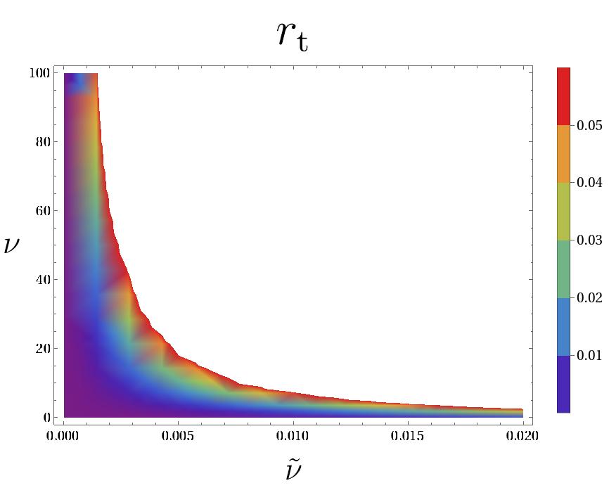
We see that the consistency relation in conventional models of inflation GARRIGA1999219, rt=−8​cs​ntr_{\rm t}=-8c_{s}n_{\rm t}, is modified in our model due to the mimetic constraint. In Fig. 3 we have presented the predictions for rt​(ν,ν~)r_{\rm t}(\nu,\tilde{\nu}) for cs=1c_{s}=1. The white areas correspond to the regions of parameter space which are not allowed due to the observational bound rt≤0.056r_{t}\leq 0.056 Akrami:2018odb. By choosing smaller values of csc_{s} the allowed regions become more extended.
Refer to caption
Figure 3: The density plot of rtr_{\rm t} versus ν\nu and ν~\tilde{\nu} for cs=1c_{s}=1. The white regions are excluded by the observational bound rt≤0.056r_{t}\leq 0.056 Akrami:2018odb.

Before closing this section, here we compare our results for the inflationary background with those of Zheng:2017qfs. We have shown that in order for a consistent inflationary solution to exist in this setup, the potential has to be negative. Then imposing the additional condition that the parameter 𝒦{\cal K} defined in Eq. (11) be a constant we have verified the existence of a period of slow-roll inflation as demonstrated in Fig. 1. Then calculating the quadratic actions and performing the perturbation analysis we have shown that the spectral tilt of tensor perturbations can take either signs. On the other hand, Ref. Zheng:2017qfs claimed the existence of slow-roll solution with a potential which is (implicitly) positive66 6 There is a discrepancy with the signature of the action used in Zheng:2017qfs. While they use the (+,−,−,−)(+,-,-,-) signature as in Chamseddine-Mukhanov Chamseddine:2013kea, but their action has an opposite sign for the Einstein-Hilbert term. Fortunately, this sign discrepancy does not affect their perturbation analysis about the ghost/gradient instabilities but it has important effects when writing the background equation. More specifically, their potential should be replaced by −V-V. . As for the predictions of the scalar and tensor power spectra they have borrowed the analysis of Fujita:2015ymn which was in a different context. As a result, they have obtained the standard result nt=−2​ϵHn_{\rm t}=-2\epsilon_{H}, so the tilt of tensor perturbations is always negative.

4 Primordial Bispectra

In this section, we calculate the three-point correlation of the scalar perturbations ⟨ℛ​ℛ​ℛ⟩\langle\mathcal{R}\mathcal{R}\mathcal{R}\rangle and look at the amplitudes and shapes of non-Gaussianity in various limits.

Utilizing the standard methods, the expectation value of the three point correlation is given by Maldacena:2002vr

⟨ℛ(𝐤1)ℛ(𝐤2)ℛ(𝐤3)⟩=−i∫τiτeadτ⟨0|[ℛ(τe,𝐤1)ℛ(τe,𝐤2)ℛ(τe,𝐤3),Hint]|0⟩,\Big\langle\mathcal{R}\left({\bf k}_{1}\right)\mathcal{R}\left({\bf k}_{2}\right)\mathcal{R}\left({\bf k}_{3}\right)\Big\rangle=-i\int_{\tau_{\rm i}}^{\tau_{\rm e}}a\ {\rm d}\tau\Big\langle 0\Big|\Big[\mathcal{R}(\tau_{\rm e},\,{\bf k}_{1})\mathcal{R}(\tau_{\rm e},\,{\bf k}_{2})\mathcal{R}(\tau_{\rm e},\,{\bf k}_{3})~,\,H_{\rm int}\Big]\Big|0\Big\rangle\,, (48)

where HintH_{\rm int} is the interaction Hamiltonian which is calculated from expanding the Lagrangian (3) up to 3rd orders in curvature perturbations, given in (A.2), with Hint=−ℒ3H_{\rm int}=-\mathcal{L}_{3}. Moreover, 𝐤i{\bf k}_{\rm i} are the wave vectors and τi\tau_{\rm i} is the initial time when the inflationary perturbations are deep inside the Hubble radius. Since during a quasi-de Sitter expansion τ≃−1/(aH)\tau\simeq-1/(aH), it is a good approximation to calculate the integral in the limit τi→−∞\tau_{\rm i}\to-\infty and τe→0\tau_{\rm e}\to 0.

In the Fourier space, we can write the three-point correlation function of curvature perturbations as

⟨ℛ⁡(𝐤1)​ℛ​(𝐤2)​ℛ​(𝐤3)⟩≡(2​π)3​δ3​(𝐤1+𝐤2+𝐤3)​ℬℛ​(k1,k2,k3),\displaystyle\Big\langle\mathcal{R}\left({\bf k}_{1}\right)\mathcal{R}\left({\bf k}_{2}\right)\mathcal{R}\left({\bf k}_{3}\right)\Big\rangle\equiv\left(2\pi\right)^{3}\delta^{3}\left({\bf k}_{1}+{\bf k}_{2}+{\bf k}_{3}\right)\ \mathcal{B}_{\mathcal{R}}\left(k_{1},k_{2},k_{3}\right)\,, (49)

in which ki=|𝐤i|k_{i}=|{\bf k}_{i}| and Bℛ​(k1,k2,k3)B_{\mathcal{R}}\left(k_{1},k_{2},k_{3}\right) is called the bispectrum 77 7 Because of the translational invariance, the total momentum 𝐊≡𝐤1+𝐤2+𝐤3{\bf K}\equiv{\bf k}_{1}+{\bf k}_{2}+{\bf k}_{3} is conserved. which can be parameterized as

Bℛ​(k1,k2,k3)≡(2​π)4​𝒫ℛ2∏n=13ki3​𝒜​(k1,k2,k3)B_{\mathcal{R}}\left(k_{1},k_{2},k_{3}\right)\equiv\frac{(2\pi)^{4}\ \mathcal{P}_{\cal R}^{2}}{\prod_{n=1}^{3}k_{i}^{3}}\mathcal{A}(k_{1},k_{2},k_{3}) (50)

where 𝒜\mathcal{A} is called the amplitude of bispectrum.

Finally, the non-linearity parameter fNLf_{{}_{\rm NL}} associated with the amplitude of bispectrum is defined by the following relation

fNL≡1031∑i=13ki3𝒜(k1,k2,k3).f_{{}_{\rm NL}}\equiv\frac{10}{3}\frac{1}{\sum_{i=1}^{3}k_{i}^{3}}\mathcal{A}\left(k_{1},k_{2},k_{3}\right)\,. (51)

As we see from Eq. (A.2), our interaction Hamiltonian contains 22 independent terms (interactions). These complicated interactions originate from the higher derivative terms in F⁡(χ)F(\chi) and P⁡(χ)P(\chi). Each of them induce different shapes and amplitudes of non-Gaussianities.

As examples, let us calculate the bispectrum for the following two terms of the cubic action (A.2),

ℒint⊃f2​ℛ˙​(∂ℛ)2a2+f8​ℛ˙3,\displaystyle{\cal L}_{\rm int}\supset f_{2}~\dot{{\cal{R}}}\dfrac{{\left(\partial{\cal{R}}\right)}^{2}}{a^{2}}+f_{8}~\dot{{\cal{R}}}^{3}\,, (52)

which also exist in the model of ghost inflation with the modified dispersion relation ω2∝k4\omega^{2}\propto k^{4}.

The bispectrum for each term in Eq. (52) is evaluated using the mode function of ℛ\mathcal{R} given in Eq. (34) as follows

ℬℛ​(k1,k2,k3)2\displaystyle\mathcal{B}_{\mathcal{R}}\left(k_{1},k_{2},k_{3}\right)_{2} =i​f2​wk1∗​(0)​wk2∗​(0)​wk3∗​(0)​∫−∞0d​τ​1H​τ​wk1​(τ)​wk2​(τ)​wk3′​(τ)​(𝐤1⋅𝐤2)\displaystyle=if_{2}\ w^{*}_{k_{1}}(0)w^{*}_{k_{2}}(0)w^{*}_{k_{3}}(0)\int_{-\infty}^{0}{\rm d}\tau\ \frac{1}{H\tau}w_{k_{1}}(\tau)w_{k_{2}}(\tau)w^{\prime}_{k_{3}}(\tau)\ ({\bf k}_{1}\cdot{\bf k}_{2}) (53)
+symm.+c.c.\displaystyle+{\rm symm.}+{\rm{c.c.}}

and

ℬℛ​(k1,k2,k3)8\displaystyle\mathcal{B}_{\mathcal{R}}\left(k_{1},k_{2},k_{3}\right)_{8} =6​i​f8​wk1∗​(0)​wk2∗​(0)​wk3∗​(0)​∫−∞0d​τ​1H​τ​wk1′​(τ)​wk2′​(τ)​wk3′​(τ)+c.c..\displaystyle=6if_{8}\ w^{*}_{k_{1}}(0)w^{*}_{k_{2}}(0)w^{*}_{k_{3}}(0)\int_{-\infty}^{0}{\rm d}\tau\frac{1}{H\tau}w^{\prime}_{k_{1}}(\tau)w^{\prime}_{k_{2}}(\tau)w^{\prime}_{k_{3}}(\tau)+{\rm{c.c.}}\,. (54)

Using the explicit expression for the wave function (34) and substituting the above results into Eq. (50) for 𝒜\mathcal{A}, we obtain the following expressions for the amplitudes 𝒜(2)\mathcal{A}^{(2)} and 𝒜(8)\mathcal{A}^{(8)} associated with each interaction:

𝒜(2)\displaystyle\mathcal{A}^{(2)} =f2​H5cs8​𝒫ℛ2​ϑ3∑i,j,l=13|ϵi​j​l|ℐ1,−1pi,pj,pl(v)ki(𝐤j.𝐤l),\displaystyle=\frac{f_{2}H^{5}}{c_{s}^{8}\mathcal{P}_{\cal R}^{2}\vartheta^{3}}\sum_{i,j,l=1}^{3}|\epsilon_{ijl}|\ \mathcal{I}^{{}^{p_{i},p_{j},p_{l}}}_{{}_{1,-1}}(v)\ k_{i}({\bf k}_{j}.{\bf k}_{l})\,, (55)

with p1=1p_{1}=1 and p2=p3=0p_{2}=p_{3}=0, and

𝒜(8)\displaystyle\mathcal{A}^{(8)} =6​f8​H5cs6​𝒫ℛ2​ϑ3k1k2k3ℐ0,−11,1,1(ν).\displaystyle=\frac{6f_{8}H^{5}}{c_{s}^{6}\mathcal{P}_{\cal R}^{2}\vartheta^{3}}k_{1}k_{2}k_{3}\ \mathcal{I}^{{}^{1,1,1}}_{{}_{0,-1}}(\nu)\,. (56)

Here the function ℐn1,n2p1,p2,p3\mathcal{I}_{{}_{n_{{}_{1}},n_{{}_{2}}}}^{{}^{p_{{}_{1}},p_{{}_{2}},p_{{}_{3}}}} is defined via

ℐn1,n2p1,p2,p3(ν,k1,k2,k3)≡Re[α(ν)ν−(n1+34)∫−∞0dxxn2hν(p1)(x)hν(p2)(k2k1x)hν(p3)(k3k1x)],\mathcal{I}^{{}^{{p_{{}_{1}},p_{{}_{2}},p_{{}_{3}}}}}_{{}_{n_{{}_{1}},n_{{}_{2}}}}(\nu,k_{1},k_{2},k_{3})\equiv\mathrm{Re}\Big[\alpha(\nu)\nu^{-(n_{1}+\frac{3}{4})}\int_{-\infty}^{0}dx\;x^{n_{2}}h^{(p_{1})}_{\nu}(x)h^{(p_{2})}_{\nu}\big(\frac{k_{2}}{k_{1}}x\big)h^{(p_{3})}_{\nu}\big(\frac{k_{3}}{k_{1}}x\big)\Big]\,, (57)

where

α⁡(ν)≡15​e(i−3)​π8​ν7680​π5/2​Γ​(54+i4​ν)−3andhν​(x)≡e−π8​ν​x​Wi4​ν,34​(−i​x2)ν3/4,\alpha(\nu)\equiv\frac{15e^{\frac{(i-3)\pi}{8\nu}}}{7680\pi^{5/2}}\Gamma\Big(\frac{5}{4}+\frac{i}{4\nu}\Big)^{-3}\hskip 14.22636pt\text{and}\hskip 14.22636pth_{\nu}(x)\equiv\frac{e^{-\frac{\pi}{8\nu}}\sqrt{x}\ W_{\frac{i}{4\nu},\frac{3}{4}}\left(-ix^{2}\right)}{\nu^{3/4}}\;, (58)

and the upper index pip_{{}_{i}} denotes the order of derivative with respect to the function variables. For example hν(0)​(x)=hν​(x),hν(1)​(x)=d​hν​(x)d​xh^{(0)}_{\nu}(x)=h_{\nu}(x),h^{(1)}_{\nu}(x)=\frac{d\,h_{\nu}(x)}{dx} and so on. The amplitudes for all other interactions are listed in Appendix B.

To study the shape function of the above amplitudes, in Figs. 4 and 5 we have presented the 3D plot of r2−1​r3−1​𝒜​(1,r2,r3)r_{2}^{-1}r_{3}^{-1}\mathcal{A}(1,r_{2},r_{3}) as a function of r2≡k2/k1r_{2}\equiv k_{2}/k_{1} and r3≡k3/k2r_{3}\equiv k_{3}/k_{2} for ν={1,10,50}\nu=\{1,10,50\}. The plots are produced numerically, after rotating the contour of integration over τ\tau along the direction ∝−(1+i)\propto-(1+i) so that they converge exponentially. We see that 𝒜(2)\mathcal{A}^{(2)} and 𝒜(8)\mathcal{A}^{(8)} roughly have similar shapes and amplitudes and both roughly peak at the equilateral limit k1=k2=k3=kk_{1}=k_{2}=k_{3}=k. In addition, the variation of ν\nu has no significant effects on the shapes.

Refer to caption
Refer to caption
Refer to caption
Figure 4: Numerical results for the shapes of |𝒜(2)|/k1​k2​k3|\mathcal{A}^{(2)}|/k_{1}k_{2}k_{3} for ν=1,10,50\nu=1,10,50 from left to right. The amplitude is normalized by the value obtained in the equilateral limit.
Refer to caption
Refer to caption
Refer to caption
Figure 5: Numerical results for the shapes of |𝒜(8)|/k1​k2​k3|\mathcal{A}^{(8)}|/k_{1}k_{2}k_{3} for ν=1,10,50\nu=1,10,50 from left to right with the description as in Fig. 4.
Refer to caption
Refer to caption
Figure 6: Numerical results for the shapes of |𝒜(4)|/k1​k2​k3|\mathcal{A}^{(4)}|/k_{1}k_{2}k_{3} (left panel) and |𝒜(10)|/k1​k2​k3|\mathcal{A}^{(10)}|/k_{1}k_{2}k_{3} (right panel) for ν=1\nu=1. The amplitude is normalized by the value obtained in the equilateral limit.
Amplitude 𝒜(1)\mathcal{A}^{(1)} 𝒜(3)\mathcal{A}^{(3)} 𝒜(4)\mathcal{A}^{(4)} 𝒜(5)\mathcal{A}^{(5)} 𝒜(6)\mathcal{A}^{(6)} 𝒜(7)\mathcal{A}^{(7)} 𝒜(9)\mathcal{A}^{(9)} 𝒜(10)\mathcal{A}^{(10)} 𝒜(11)\mathcal{A}^{(11)} 𝒜(12)\mathcal{A}^{(12)}
Shape Local Equi Local Equi Equi Local Equi Ortho Equi Equi
Amplitude 𝒜(13)\mathcal{A}^{(13)} 𝒜(14)\mathcal{A}^{(14)} 𝒜(15)\mathcal{A}^{(15)} 𝒜(16)\mathcal{A}^{(16)} 𝒜(17)\mathcal{A}^{(17)} 𝒜(18)\mathcal{A}^{(18)} 𝒜(19)\mathcal{A}^{(19)} 𝒜(20)\mathcal{A}^{(20)} 𝒜(21)\mathcal{A}^{(21)} 𝒜(22)\mathcal{A}^{(22)}
Shape Equi Local Equi Equi Equi Equi Equi Equi Ortho Equi
Table 1: The shape of bispectrum for each interaction listed in Appendix. B.

In Table 1 we list the shape of each contribution presented in Appendix B. One can see that most of the non-Gaussianity shapes peak at the equilateral limit where all three modes have comparable wavelengths. However, some shapes are close to the orthogonal shape and the local shape which has a peak in the squeezed limit. For example, as shown in Fig. 6, 𝒜(4)\mathcal{A}^{(4)} and 𝒜(10)\mathcal{A}^{(10)} peak in the squeezed triangle limit (k3≪k1≃k2k_{3}\ll k_{1}\simeq k_{2}) and in orthogonal triangle limit (k3=k2=k1/2k_{3}=k_{2}=k_{1}/2), respectively.

Combining the contributions from all interactions listed in Appendix B, the total non-Gaussianity parameter fNLf_{{}_{\rm NL}} is given by

fNL=1031∑i=13ki3∑j=122𝒜(j).f_{{}_{\rm NL}}=\frac{10}{3}\frac{1}{\sum_{i=1}^{3}k_{i}^{3}}\sum_{j=1}^{22}\mathcal{A}^{(j)}\,. (59)

Correspondingly, we can calculate fNLf_{{}_{\rm NL}} numerically for squeezed (k1=k2=k,k3→0)(k_{1}=k_{2}=k,k_{3}\to 0), equilateral (k1=k2=k3=kk_{1}=k_{2}=k_{3}=k) and orthogonal (k1=k,k2=k3=k/2)k_{1}=k,k_{2}=k_{3}=k/2) shapes.

In Figs. 7, 8, and 9, fNLf_{{}_{\rm NL}} is presented in the various range of ν\nu in the squeezed, equilateral and orthogonal configurations. It is worth mentioning that fNLf_{{}_{\rm NL}} is controlled by three parameters, the sound speed csc_{s}, the scalar to tensor ratio rtr_{\rm t} and ν\nu. In the left hand panels of these figures, fNLf_{{}_{\rm NL}} can take the observationally allowed values in some range of ν\nu by varying csc_{s} while rt=0.01r_{\rm t}=0.01 is held fixed. A similar conclusion holds in the right hand panels where we fix cs=1c_{s}=1 and vary rtr_{\rm t}. Generally, fNLf_{{}_{\rm NL}} increases by reducing csc_{s} and rtr_{\rm t}. One can find corners of parameter space which yield to acceptable amplitudes for fNLf_{{}_{\rm NL}} as required by observations in Eq. (2).

Figure 7: Numerical results for fNLf_{{}_{\rm NL}} in the equilateral configuration with ν\nu in the range [0.01,100][0.01,100]. In the left panels we have fixed cs=1c_{s}=1 while rtr_{\rm t} is varied whereas in the right panels we have set rt=0.01r_{\rm t}=0.01 and csc_{s} is varied.
Figure 8: Numerical results for fNLf_{{}_{\rm NL}} in the range of ν=[0.01,100]\nu=[0.01,100] for orthogonal configuration. In the left panels we have considered cs=1c_{s}=1, whereas in the right panels we have set rt=0.01r_{\rm t}=0.01.
Figure 9: Numerical results for fNLf_{{}_{\rm NL}} in the range of ν=[0.01,100]\nu=[0.01,100] for squeezed configuration. In the left panels we have considered cs=1c_{s}=1, whereas in the right panels we have set rt=0.01r_{\rm t}=0.01.

For further studies of bispectrum and its expansion in terms of slow-roll parameters see Appendix B.1.

5 Summaries and Conclusions

In this paper we have studied inflationary solution in an extension of mimetic gravity with higher derivative interactions coupled to gravity. It is known that the original mimetic setup is plagued with the ghost and gradient instabilities. These instabilities can be removed with the help of higher derivative interactions coupled to gravity. There are a number of options to include higher derivative corrections. In this paper we have studied the simplest higher derivative correction in the form F⁡(χ)​RF(\chi)R with χ≡□​ϕ\chi\equiv\Box\phi. It would be interesting to extend the current analysis to include other higher derivative terms coupled to gravity such as F2​(∇μ∇ν​ϕ​Rμ​ν)F_{2}(\nabla_{\mu}\nabla_{\nu}\phi R^{\mu\nu}), F3​(χ​∇μϕ​∇νϕ​Rμ​ν)F_{3}(\chi\nabla_{\mu}\phi\nabla_{\nu}\phi R^{\mu\nu}) etc. In addition, in order for the scalar perturbations to become dynamical with a non-zero sound speed csc_{s} we have included the term P⁡(χ)P(\chi) as well.

One curious effect in our analysis is that in order to obtain an inflationary solution we have to work with a negative potential. This conclusion is a consequence of the fact that we deal with a constrained theory. More specifically, in oder for the quadratic actions of the scalar and tensor perturbation to be free from instabilities the higher derivative functions F⁡(χ)F(\chi) and P⁡(χ)P(\chi) are subject to certain conditions which cause the potential to be negative. Inflation is achieved while the field rolls up the potential towards V=0V=0. While a negative potential may be considered problematic a priori but our analysis show that the setup shows no pathologies either at the background or at the perturbation level.

While the background yields a period of slow-roll inflation the cosmological perturbations in this setup have novel behaviours. Because of the higher derivative interactions the dispersion relation associated with the scalar perturbations receives higher order momentum corrections as in the model of ghost inflation. Furthermore, the tilt of tensor perturbations can take either signs in contrast to conventional inflation models Maldacena:2002vr; Acquaviva:2002ud. In addition, we obtain a new consistency relation between rtr_{\rm t} and ntn_{\rm t} which involves csc_{s} and other model parameters encoding the higher derivative interactions. Despite the presence of higher derivative corrections the tensor perturbations propagate with the speed equal to speed of light as strongly implied by the LIGO observations.

We also studied the predictions of this setup for the amplitudes and shapes of non-Gaussianities. Because of higher derivative interactions, various types of interactions are developed in the cubic action endowing the setup with rich non-Gaussianity properties. Depending on model parameters, large amplitudes of non-Gaussianities in various shapes such as equilateral, orthogonal and squeezed configurations are produced.

As we mentioned before, it is assumed that the effective Newton constant is stabilized after inflation, corresponding to F⁡(χe)=1F(\chi_{e})=1. We did not provide a dynamical mechanism for this important requirement. In addition, we have not specified the reheating mechanism in this setup. Indeed, it is possible that these two questions are related to each other. While this work was primarily concerned with cosmological perturbations such as the power spectrum and bispectrum, but a concrete picture requires that the questions of reheating and the stabilization of the effective Newton constant to be addressed as well. These are important questions which are beyond the scope of the current analysis.

Acknowledgements

We would like to thank Alireza Vafaei Sadr, Amin Farhang and Mehdi Atashi for helpful discussions on the numerical methods and Mohammad Ali Gorji for insightful discussions.

Appendix A Cosmological perturbations

In this Appendix we present the analysis of cosmological perturbations in comoving gauge in which the calculations are significantly simpler than other gauges. Moreover, this gauge is especially suitable for investigating the ghost and gradient instabilities. The special property of this gauge is that all perturbation are encoded in the metric sector while the scalar field is kept unperturbed, δ​ϕ​(t,x→)=0\delta\phi(t,\vec{x})=0.

Implementing the ADM formalism, the metric is decomposed as

d​s2=−N2​d​t2+hi​j​(d​xi+Ni​d​t)​(d​xj+Nj​d​t),{\rm d}s^{2}=-N^{2}{\rm d}t^{2}+h_{ij}({\rm d}x^{i}+N^{i}{\rm d}t)({\rm d}x^{j}+N^{j}{\rm d}t)~\,, (60)

in which NN and NiN^{i} are the lapse function and the shift vector respectively while the three-dimensional metric hi​jh_{ij} determines the geometry of the spatial hypersurfaces. At the level of background N=1N=1, Ni=0N_{i}=0 and hi​j=a​(t)2​δi​jh_{ij}=a(t)^{2}\delta_{ij}. It is then possible to write down perturbations as follows,

N≡1+α,Ni≡∂iψ,hi​j≡a​(t)2​e2​ℛ​δi​j+γi​j,N\equiv 1+\alpha\,,\hskip 14.22636ptN_{i}\equiv\partial_{i}\psi\,,\hskip 14.22636pth_{ij}\equiv a(t)^{2}e^{2\mathcal{R}}\delta_{ij}+\gamma_{ij}\,, (61)

where α\alpha, ψ\psi and ℛ\mathcal{R} are scalar perturbations. In addition, there is the scalar perturbation λ=λ⁡(t)+δ​λ​(t,x→)\lambda=\lambda(t)+\delta\lambda(t,\vec{x}) for the Lagrange multiplier.

Because of the global O⁡(3)O(3) symmetry, the scalar, vector and tensor perturbations decouple at the linear order of perturbations. Here we have ignored vector perturbations in Eq. (61) in view of the fact that the vector perturbations decay as usual in an expanding universe.

At this stage, the above perturbations must be substituted in the action (3) to extract the quadratic and cubic actions for the scalar and tensor perturbations. Before doing so, let us first impose the mimetic constraint Eq. (1) at the level of perturbations defined in Eq. (61) which yields

α=0.\displaystyle\alpha=0\,. (62)

This result simplifies our following calculations considerably.

A.1 Linear perturbations: Quadratic action

Plugging the above perturbations into the action (3) and after some integration by parts, the quadratic action in comoving gauge for ℛ{\cal{R}} and γi​j\gamma_{ij} is obtained as follows

Scom(2)\displaystyle S^{(2)}_{\rm com} =\displaystyle= ∫dtd3xa32{−3(F+152HFχ−9H2Fχ​χ)(ℛ˙2+ℛℛ˙)−3𝒦ℛℛ˙−2Fχ∂2ψ∂2ℛ\displaystyle\int{\rm d}t\,{\rm d}^{3}\textbf{x}\ \frac{a^{3}}{2}\Bigg\{-3\Big(F+\frac{15}{2}HF_{\chi}-9H^{2}F_{\chi\chi}\Big)\Big(\dot{{\cal{R}}}^{2}+{\cal{R}}\dot{{\cal{R}}}\Big)-3{\mathcal{K}}{\cal{R}}\dot{{\cal{R}}}-2F_{\chi}~\partial^{2}\psi~\partial^{2}{\cal{R}} (63)
+(∂ℛ)2a2​(F+3​H​Fχ−9​H˙​Fχ​χ)−2​𝒦​∂2ψ​ℛ˙+13​(∂2ψ)2​(𝒦+F)\displaystyle+\frac{{{\left(\partial{\cal{R}}\right)}^{2}}}{{a^{2}}}\big(F+3HF_{\chi}-9\dot{H}F_{\chi\chi}\big)-2{\mathcal{K}}\ \partial^{2}\psi~\dot{{\cal{R}}}+\dfrac{1}{3}\left(\partial^{2}\psi\right)^{2}\left({\mathcal{K}}+F\right)
+\displaystyle+ F4[(γ˙i​j)2−(∂γi​j)2a2]}\displaystyle\frac{F}{4}\Big[(\dot{\gamma}_{ij})^{2}-\dfrac{(\partial\gamma_{ij})^{2}}{a^{2}}\Big]\Bigg\}\,

where we have used Eq. (11) to simplify the result in terms of the function 𝒦{\mathcal{K}}. Note that in the these analysis there is no assumption on the function 𝒦{\mathcal{K}} so it is kept general.

It is evident that the ψ\psi mode is a non dynamical degrees of freedom which can be integrated out from the action. Varying Eq. (63) with respect to ψ\psi, we find

∂2ψ=3𝒦+F​(𝒦​ℛ˙+Fχ​∂2ℛa2).\displaystyle\partial^{2}\psi=\dfrac{3}{{\mathcal{K}}+F}\Big({\mathcal{K}}\ \dot{{\cal{R}}}+F_{\chi}\ \dfrac{\partial^{2}{\cal{R}}}{a^{2}}\Big)\,. (64)

Substituting the above result into the action (63) and after some integration by parts the quadratic Lagrangian in comoving gauge for ℛ\mathcal{R} and γi​j\gamma_{ij} is obtained to be

ℒ2\displaystyle{\cal L}_{2} =\displaystyle= ϑ​a32​{ℛ˙2−cs2a2​(∂ℛ)2−σ2​(∂2ℛa2)2+F4​ϑ​[(γ˙i​j)2−(∂γi​j)2a2]},\displaystyle\vartheta\frac{a^{3}}{2}\left\{\dot{{\cal{R}}}^{2}-\frac{c_{s}^{2}}{a^{2}}{{\big(\partial{\cal{R}}\big)}^{2}}-\sigma^{2}\Big(\dfrac{\partial^{2}{\cal{R}}}{a^{2}}\Big)^{2}+\frac{F}{4\vartheta}\left[(\dot{\gamma}_{ij})^{2}-\dfrac{(\partial\gamma_{ij})^{2}}{a^{2}}\right]\right\}\,, (65)

in which we have defined

ϑ≡3​𝒦​F𝒦+F,σ2≡Fχ2𝒦​F,\displaystyle\vartheta\equiv\dfrac{3{\mathcal{K}}\,F}{{\mathcal{K}}+F},\hskip 28.45274pt\sigma^{2}\equiv\dfrac{F^{2}_{\chi}}{{\mathcal{K}}\,F}\,, (66)

and during inflation, the sound speed of the scalar perturbations cs2c_{s}^{2} as

cs2\displaystyle c_{s}^{2} ≡−13​𝒦​(𝒦+F+3​H​Fχ).\displaystyle\equiv-\dfrac{1}{3{\mathcal{K}}}\left({\mathcal{K}}+F+3HF_{\chi}\right)\,. (67)

As discussed in the main text, in order to avoid the ghost and gradient instabilities we demand that ϑ>0,cs2>0\vartheta>0,\ c_{s}^{2}>0 and σ2>0\sigma^{2}>0. Applying these conditions on Eqs. (66) and (67), we obtain the following constraints

𝒦>0,F>0,Fχ<0.\displaystyle{\mathcal{K}}>0\,,~~~~~~~~~~F>0\,,~~~~~~~~~~F_{\chi}<0\ . (68)

A.2 Nonlinear scalar perturbations: Cubic action

In this section, we calculate the cubic action for the scalar perturbations which is used to calculate the bispectrum.

Expanding the action (3) up to third order, the cubic action is given by

Scom(3)\displaystyle S^{(3)}_{\rm com} =\displaystyle= ∫dtd3xa3{9𝒦ℛℛ˙2+f~1ℛ(∂ℛ)2a2−9Fχ​χℛ˙2∂2ℛa2−6𝒦(ℛ˙∂iℛ∂iψ+ℛℛ˙∂2ψ)\displaystyle\int{\rm d}t\,{\rm d}^{3}x\ a^{3}\Big\{9{\mathcal{K}}~{\cal{R}}\dot{{\cal{R}}}^{2}+\tilde{f}_{1}~{\cal R}\dfrac{{\left(\partial{\cal{R}}\right)}^{2}}{a^{2}}-9F_{\chi\chi}~\dot{{\cal{R}}}^{2}\dfrac{\partial^{2}{\cal{R}}}{a^{2}}-6{\mathcal{K}}\left(\dot{\cal R}\ \partial_{i}{\cal{R}}\ \partial_{i}\psi+{\cal{R}}\dot{{\cal{R}}}\ \partial^{2}\psi\right) (69)
−\displaystyle- 6​Fχ​∂iℛ​∂iψ​∂2ℛa2+2​𝒦​∂iℛ​∂iψ​∂2ψ−Fχ​(∂ℛ)2a2​∂2ψ+12​(f~2​ℛ−f~3​ℛ˙)​(∂2ψ)2\displaystyle 6F_{\chi}\ \partial_{i}{\cal{R}}\ \partial_{i}\psi\ \dfrac{\partial^{2}{\cal{R}}}{a^{2}}+2{\mathcal{K}}\ \partial_{i}{\cal{R}}\ \partial_{i}\psi\ \partial^{2}\psi-F_{\chi}\ \dfrac{\left(\partial{\cal{R}}\right)^{2}}{a^{2}}\ \partial^{2}\psi+\dfrac{1}{2}\left(\tilde{f}_{2}\ {\cal{R}}-\tilde{f}_{3}\ \dot{{\cal{R}}}\right)\left(\partial^{2}\psi\right)^{2}
−\displaystyle- 2​(Fχ​ℛ−3​Fχ​χ​ℛ˙)​∂2ℛa2​∂2ψ+32​(F​ℛ−Fχ​ℛ˙)​∂i∂jψ​∂i∂jψ−Fχ​χ​∂2ℛa2​(∂2ψ)2\displaystyle 2\left(F_{\chi}\ {\cal{R}}\ -3F_{\chi\chi}\ \dot{{\cal{R}}}\right)\dfrac{\partial^{2}{\cal{R}}}{a^{2}}\ \partial^{2}\psi+\dfrac{3}{2}\left(F\ {\cal{R}}-F_{\chi}\ \dot{{\cal{R}}}\right)\partial_{i}\partial_{j}\psi\ \partial_{i}\partial_{j}\psi-F_{\chi\chi}\ \dfrac{\partial^{2}{\cal{R}}}{a^{2}}\ \left(\partial^{2}\psi\right)^{2}
−3(2Fχ​χ−3HFχ​χ​χ)ℛ˙∂2ψ∂2ψ˙},\displaystyle-3\left(2F_{\chi\chi}-3HF_{\chi\chi\chi}\right)\dot{{\cal{R}}}\ \partial^{2}\psi\ \partial^{2}\dot{\psi}\Big\}\,,

where, using the definition of 𝒦\mathcal{K} in Eq. (11), the coefficients f~i\tilde{f}_{i} are given by

f~1\displaystyle\tilde{f}_{1} ≡F+3HFχ+9H2ϵHFχ​χ\displaystyle\equiv F+3HF_{\chi}+9H^{2}\epsilon_{{}_{H}}F_{\chi\chi} (70)
f~2\displaystyle\tilde{f}_{2} ≡2𝒦−F−9HFχ+9H2Fχ​χ(3−2ϵH)+27H3Fχ​χ​χϵH\displaystyle\equiv 2{\mathcal{K}}-F-9HF_{\chi}+9H^{2}F_{\chi\chi}(3-2\epsilon_{{}_{H}})+27H^{3}F_{\chi\chi\chi}\epsilon_{{}_{H}} (71)
f~3\displaystyle\tilde{f}_{3} ≡2​Fχ−9​H​Fχ​χ\displaystyle\equiv 2F_{\chi}-9HF_{\chi\chi} (72)

The next step is to eliminate ψ\psi in the above action by utilizing Eq. (64). To do this, let us define ∂2Ξ≡Q2​ℛ˙\partial^{2}\Xi\equiv Q_{2}\dot{{\cal{R}}} in which Q2≡3​ν~2/(1+ν~2)Q_{2}\equiv 3\tilde{\nu}^{2}/(1+\tilde{\nu}^{2}) with ν~=𝒦/F\tilde{\nu}=\sqrt{{\mathcal{K}}/{F}}. This definition provides us with the contributions proportional to the linear differential equation of ℛ\mathcal{R}, i.e.,

δ​ℒ2δ​ℛ|1=−[∂t(ϑ​a3​ℛ˙)−ϑ​a​cs2​∂2ℛ+ϑ​σ2a​∂4ℛ],\dfrac{\delta{\cal L}_{2}}{\delta{\cal R}}\biggr|_{1}=-\left[\partial_{t}\left(\vartheta a^{3}\dot{{\cal{R}}}\right)-\vartheta ac_{s}^{2}\,\,\partial^{2}{\cal{R}}+\dfrac{\vartheta\sigma^{2}}{a}\,\partial^{4}{\cal{R}}\right]\,, (73)

in the final cubic action. Substituting the relation

ψ=Q1H​ℛa2+Ξ,Q1≡−1−cs2​Q2\displaystyle\psi=\dfrac{Q_{1}}{H}\,\dfrac{{\cal{R}}}{a^{2}}+\Xi\,,\quad\quad Q_{1}\equiv-1-c_{s}^{2}Q_{2} (74)

into the action (69) and performing a lot of integrations by parts and dropping the total derivative terms88 8 The integration by parts relations presented in Ref. DeFelice:2011zh are useful in simplifying the calculations of the cubic action., the corresponding cubic Lagrangian is obtained to be

ℒ3a3\displaystyle\dfrac{{\cal L}_{3}}{a^{3}} =f1​ℛ​(∂ℛ)2a2+f2​ℛ˙​(∂ℛ)2a2+f3​ℛ˙2​∂2ℛa2+f4​ℛ​(∂2ℛa2)2+f5​ℛ˙​(∂2ℛa2)2\displaystyle=f_{1}~{\cal R}\dfrac{{\big(\partial{\cal{R}}\big)}^{2}}{a^{2}}+f_{2}~\dot{{\cal{R}}}\dfrac{{\big(\partial{\cal{R}}\big)}^{2}}{a^{2}}+f_{3}~\dot{{\cal{R}}}^{2}\dfrac{\partial^{2}{\cal{R}}}{a^{2}}+f_{4}~{\cal{R}}\big(\dfrac{\partial^{2}{\cal{R}}}{a^{2}}\big)^{2}+f_{5}~\dot{{\cal{R}}}\big(\dfrac{\partial^{2}{\cal{R}}}{a^{2}}\big)^{2}
+f6​(∂2ℛa2)3+f7​ℛ​ℛ˙2+f8​ℛ˙3+f9​∂2ℛa2​(∂ℛ)2a2+f10​ℛ˙​∂2ℛ˙a2​∂2ℛa2\displaystyle+f_{6}~\big(\dfrac{\partial^{2}{\cal{R}}}{a^{2}}\big)^{3}+f_{7}~{\cal{R}}\dot{{\cal{R}}}^{2}+f_{8}~\dot{{\cal{R}}}^{3}+f_{9}~\dfrac{\partial^{2}{\cal{R}}}{a^{2}}\dfrac{{\big(\partial{\cal{R}}\big)}^{2}}{a^{2}}+f_{10}~\dot{{\cal{R}}}\,\dfrac{\partial^{2}\dot{{\cal{R}}}}{a^{2}}\,\dfrac{\partial^{2}{\cal{R}}}{a^{2}}
+f11​ℛ˙2​∂2ℛ˙a2+f12​(∂ℛa)2​∂4ℛa4+f13​(∂ℛa)2​∂2ℛ˙a2+f14​∂iℛa​∂i∂jΞ​∂jℛa\displaystyle+f_{11}~\dot{{\cal{R}}}^{2}\dfrac{\partial^{2}\dot{{\cal{R}}}}{a^{2}}+f_{12}~\big(\dfrac{\partial{\cal{R}}}{a}\big)^{2}\dfrac{\partial^{4}{\cal{R}}}{a^{4}}+f_{13}~\big(\dfrac{\partial{\cal{R}}}{a}\big)^{2}\dfrac{\partial^{2}\dot{{\cal{R}}}}{a^{2}}+f_{14}~\dfrac{\partial_{i}{\cal{R}}}{a}\,\partial^{i}\partial^{j}\Xi\,\dfrac{\partial_{j}{\cal{R}}}{a}
+f15∂2ℛa2∂iℛ∂iΞ+f16ℛ˙∂iℛ∂iΞ+f17∂4ℛa4∂iℛ∂iΞ+f18∂2ℛ(∂Ξ)2\displaystyle+f_{15}~\dfrac{\partial^{2}{\cal{R}}}{a^{2}}\partial_{i}{\cal{R}}\,\partial^{i}\Xi+f_{16}\dot{{\cal{R}}}\,\partial_{i}{\cal{R}}\,\partial^{i}\Xi+f_{17}\dfrac{\partial^{4}{\cal{R}}}{a^{4}}\,\partial_{i}{\cal{R}}\,\partial^{i}\Xi+f_{18}\partial^{2}{\cal{R}}\big(\partial\Xi\big)^{2}
+f19∂2ℛ˙a2∂iℛ∂iΞ+f20∂2ℛa2∂iℛ˙∂iΞ+f21∂2ℛa2∂i∂jΞ∂i∂jℛa2+f22∂4ℛa2(∂Ξ)2\displaystyle+f_{19}~\dfrac{\partial^{2}\dot{{\cal{R}}}}{a^{2}}\,\partial_{i}{\cal{R}}\,\partial^{i}\Xi+f_{20}~\dfrac{\partial^{2}{\cal{R}}}{a^{2}}\,\partial_{i}\dot{{\cal{R}}}\,\partial^{i}\Xi+f_{21}~\dfrac{\partial^{2}{\cal{R}}}{a^{2}}\,\partial_{i}\partial_{j}\Xi\,\dfrac{\partial^{i}\partial^{j}{\cal{R}}}{a^{2}}+f_{22}~\dfrac{\partial^{4}{\cal{R}}}{a^{2}}\big(\partial\Xi\big)^{2}
+ℱ​δ​ℒ2δ​ℛ|1.\displaystyle+{\cal F}~\dfrac{\delta{\cal L}_{2}}{\delta{\cal{R}}}\biggr|_{1}\,. (75)

in which the coefficient in front of δ​ℒ2/δ​R|1\delta\mathcal{L}_{2}/\delta{R}|_{1} is

ℱ≡ϵFϵH​[Q2−33​H​(2​Q2​ℛ​ℛ˙−∂−2∂i∂j(∂iℛ​∂jΞ)+3​∂iℛ​∂iΞ)−Q1​κa2​H2​∂−2∂i∂j(∂iℛ​∂jℛ)].{\cal F}\equiv\dfrac{\epsilon_{{}_{F}}}{\epsilon_{{}_{H}}}\bigg[\dfrac{Q_{2}-3}{3H}\big(2Q_{2}{\cal{R}}\dot{{\cal{R}}}-\partial^{-2}\partial^{i}\partial^{j}\big(\partial_{i}{\cal{R}}\partial_{j}\Xi\big)+3\partial_{i}{\cal{R}}\,\partial^{i}\Xi\big)-\dfrac{Q_{1}\kappa}{a^{2}H^{2}}\partial^{-2}\partial^{i}\partial^{j}\big(\partial_{i}{\cal{R}}\partial_{j}{\cal{R}}\big)\bigg]\,.

Here ∂−2\partial^{-2} is the inverse Laplacian and κ≡ϵF/ϵH+ϵF(2)/ϵH−ϵH(2)/ϵH\kappa\equiv\epsilon_{F}/\epsilon_{H}+\epsilon_{{}_{F}}^{{}^{(2)}}/\epsilon_{H}-\epsilon_{{}_{H}}^{{}^{(2)}}/\epsilon_{H}. Clearly, all contributions in ℱ\mathcal{F} include time and spatial derivatives of ℛ\mathcal{R} which vanishes in the large-scale limit (k→0k\to 0). When we calculate the bispectrum, we neglect the last term in cubic Lagrangian (A.2) relative to those coming from other terms. The other coefficients are given by

f1\displaystyle f_{1} =\displaystyle= 𝒦ν~2{1+Q1Q2(1−ϵFϵH)(1+ϵQ1+ϵQ2)+13ϵF(1+κ)(3−4Q2+Q22(1+Q1))\displaystyle\dfrac{\mathcal{K}}{\tilde{\nu}^{2}}\Big\{1+Q_{1}Q_{2}\big(1-\dfrac{\epsilon_{{}_{F}}}{\epsilon_{{}_{H}}}\big)\big(1+\epsilon_{Q_{1}}+\epsilon_{Q_{2}}\big)+\dfrac{1}{3}\epsilon_{{}_{F}}\big(1+\kappa\big)\big(3-4Q_{2}+Q_{2}^{2}\big(1+Q_{1}\big)\big) (76)
+\displaystyle+ 13ϵFϵH𝒟1+ϵHQ1Q2(1−ϵFϵHκ)+Q1​Q22ϵF((4+ϵQ1+ϵQ2)𝒞1+𝒞2ϵH)}\displaystyle\dfrac{1}{3}\dfrac{\epsilon_{{}_{F}}}{\epsilon_{{}_{H}}}{\cal D}_{1}+\epsilon_{{}_{H}}Q_{1}Q_{2}\big(1-\dfrac{\epsilon_{{}_{F}}}{\epsilon_{{}_{H}}}\kappa\big)+\dfrac{Q_{1}Q_{2}}{2}\epsilon_{{}_{F}}\Big(\big(4+\epsilon_{Q_{1}}+\epsilon_{Q_{2}}\big){\cal C}_{1}+{\cal C}_{2}\epsilon_{{}_{H}}\Big)\Big\}
−\displaystyle- 3𝒦Q1(1+ϵH+ϵQ1)+𝒦Q1Q2(1+ϵH+ϵQ1+ϵQ2),\displaystyle 3{\mathcal{K}}Q_{1}\big(1+\epsilon_{{}_{H}}+\epsilon_{Q_{1}}\big)+{\mathcal{K}}Q_{1}Q_{2}\big(1+\epsilon_{{}_{H}}+\epsilon_{Q_{1}}+\epsilon_{Q_{2}}\big)\,,
f2\displaystyle f_{2} =\displaystyle= 𝒦H(Q1+Q26​ν~2ϵFϵH)(Q2−3)+𝒦​Q1​Q22​H​ν~2{1−ϵFϵH(2+3ϵFϵH+3ϵF(2)ϵH−3ϵH(2)ϵH+Q23)\displaystyle\dfrac{{\mathcal{K}}}{H}\big(Q_{1}+\dfrac{Q_{2}}{6\tilde{\nu}^{2}}\dfrac{\epsilon_{{}_{F}}}{\epsilon_{{}_{H}}}\big)\big(Q_{2}-3\big)+\dfrac{{\mathcal{K}}Q_{1}Q_{2}}{2H\tilde{\nu}^{2}}\Big\{1-\dfrac{\epsilon_{{}_{F}}}{\epsilon_{{}_{H}}}\big(2+3\dfrac{\epsilon_{{}_{F}}}{\epsilon_{{}_{H}}}+3\dfrac{\epsilon_{{}_{F}}^{{}_{(2)}}}{\epsilon_{{}_{H}}}-3\dfrac{\epsilon_{{}_{H}}^{{}_{(2)}}}{\epsilon_{{}_{H}}}+\dfrac{Q_{2}}{3}\big)
+\displaystyle+ 𝒞3ϵH},\displaystyle{\cal C}_{3}\ \epsilon_{{}_{H}}\Big\}\,,
f3\displaystyle f_{3} =\displaystyle= 𝒦36​H2​ν~2ϵFϵH{Q1Q2(3(Q2−5)+36κ+6B(−5−ϵH+ϵQ1+ϵQ2))+6𝒞4ϵH\displaystyle\dfrac{\mathcal{K}}{36H^{2}\tilde{\nu}^{2}}\dfrac{\epsilon_{{}_{F}}}{\epsilon_{{}_{H}}}\Big\{Q_{1}Q_{2}\Big(3\big(Q_{2}-5\big)+36\kappa+6B\big(-5-\epsilon_{{}_{H}}+\epsilon_{Q_{1}}+\epsilon_{Q_{2}}\big)\Big)+6\,{\cal C}_{4}\epsilon_{{}_{H}}
−\displaystyle- 4(1+κ)(Q2−3)2},\displaystyle 4\big(1+\kappa\big)\big(Q_{2}-3\big)^{2}\Big\}\,,
f4\displaystyle f_{4} =\displaystyle= 𝒦​Q12H2(1+1ν~2)+𝒦​Q118​H2​ν~2{3(9Q1κ−4)ϵFϵH+9Q1ϵF(4κ2+2κ(1−ϵF(2)ϵH)−𝒞1)\displaystyle\dfrac{{\mathcal{K}}Q_{1}^{2}}{H^{2}}\big(1+\dfrac{1}{\tilde{\nu}^{2}}\big)+\dfrac{{\mathcal{K}}Q_{1}}{18H^{2}\tilde{\nu}^{2}}\Big\{3\big(9Q_{1}\kappa-4\big)\dfrac{\epsilon_{{}_{F}}}{\epsilon_{{}_{H}}}+9Q_{1}\epsilon_{{}_{F}}\big(4\kappa^{2}+2\kappa\big(1-\dfrac{\epsilon_{{}_{F}}^{{}_{(2)}}}{\epsilon_{{}_{H}}}\big)-{\cal C}_{1}\big)
−\displaystyle- 2Q2(ϵFϵH)2[Q2ϵQ2+(Q2−3)(−1+ϵQ1+ϵQ2+ϵH(3+2κ−ϵFϵH))]},\displaystyle 2Q_{2}\big(\dfrac{\epsilon_{{}_{F}}}{\epsilon_{{}_{H}}}\big)^{2}\big[Q_{2}\epsilon_{Q_{2}}+\big(Q_{2}-3\big)\big(-1+\epsilon_{Q_{1}}+\epsilon_{Q_{2}}+\epsilon_{{}_{H}}\big(3+2\kappa-\dfrac{\epsilon_{{}_{F}}}{\epsilon_{{}_{H}}}\big)\big)\big]\Big\}\,,
f5\displaystyle f_{5} =\displaystyle= 𝒦​Q118​H3​ν~2ϵFϵH{(Q2−3)(Q2ϵFϵH−4(1+κ))+6Q1(4κ2+2κ(1−ϵF(2)ϵH)−𝒞1)\displaystyle\dfrac{{\mathcal{K}}Q_{1}}{18H^{3}\tilde{\nu}^{2}}\dfrac{\epsilon_{{}_{F}}}{\epsilon_{{}_{H}}}\Big\{\big(Q_{2}-3\big)\big(Q_{2}\dfrac{\epsilon_{{}_{F}}}{\epsilon_{{}_{H}}}-4\big(1+\kappa\big)\big)+6Q_{1}\big(4\kappa^{2}+2\kappa\big(1-\dfrac{\epsilon_{{}_{F}}^{{}_{(2)}}}{\epsilon_{{}_{H}}}\big)-{\cal C}_{1}\big)
−\displaystyle- 3Q1(2−3κ)},\displaystyle 3Q_{1}\big(2-3\kappa\big)\Big\}\,,
f6=−𝒦​Q129​H4​ν~2​ϵFϵH​(1+κ+32​(ϵFϵH)​κ−Q14),\displaystyle f_{6}=-\dfrac{{\mathcal{K}}Q_{1}^{2}}{9H^{4}\tilde{\nu}^{2}}\ \dfrac{\epsilon_{{}_{F}}}{\epsilon_{{}_{H}}}\big(1+\kappa+\dfrac{3}{2}\big(\dfrac{\epsilon_{{}_{F}}}{\epsilon_{{}_{H}}}\big)\kappa-\dfrac{Q_{1}}{4}\big)\,,
f7\displaystyle f_{7} =\displaystyle= 𝒦​Q22​ν~2{18ϵFϵH+2Q2+Q2(ϵFϵH)2(ϵF(2)ϵH−ϵF(3)ϵH)ϵH+13ϵFϵHQ22(6−(ϵH(1+κ)+ϵQ2))}\displaystyle\dfrac{{\mathcal{K}}Q_{2}}{2\tilde{\nu}^{2}}\Big\{18\dfrac{\epsilon_{{}_{F}}}{\epsilon_{{}_{H}}}+2Q_{2}+Q_{2}\big(\dfrac{\epsilon_{{}_{F}}}{\epsilon_{{}_{H}}}\big)^{2}\big(\dfrac{\epsilon_{{}_{F}}^{{}_{(2)}}}{\epsilon_{{}_{H}}}-\dfrac{\epsilon_{{}_{F}}^{{}_{(3)}}}{\epsilon_{{}_{H}}}\big)\epsilon_{{}_{H}}+\dfrac{1}{3}\dfrac{\epsilon_{{}_{F}}}{\epsilon_{{}_{H}}}Q_{2}^{2}\big(6-\big(\epsilon_{{}_{H}}\big(1+\kappa\big)+\epsilon_{Q_{2}}\big)\big)\Big\}
+\displaystyle+ 𝒦(Q2−3)2+23(ϵFϵH)2Q22(Q2−3)ϵH,\displaystyle{\mathcal{K}}\big(Q_{2}-3\big)^{2}+\dfrac{2}{3}\big(\dfrac{\epsilon_{{}_{F}}}{\epsilon_{{}_{H}}}\big)^{2}Q_{2}^{2}\big(Q_{2}-3\big)\epsilon_{{}_{H}}\,,
f8\displaystyle f_{8} =\displaystyle= −𝒦​Q229​H​ν~2ϵFϵH{3−92κ−Q2+(3−ϵQ2)(4κ2+2κ(1−ϵF(2)ϵH)−𝒞1)+𝒞8ϵH},\displaystyle-\dfrac{{\mathcal{K}}Q_{2}^{2}}{9H\tilde{\nu}^{2}}\dfrac{\epsilon_{{}_{F}}}{\epsilon_{{}_{H}}}\Big\{3-\dfrac{9}{2}\kappa-Q_{2}+\big(3-\epsilon_{Q_{2}}\big)\big(4\kappa^{2}+2\kappa\big(1-\dfrac{\epsilon_{{}_{F}}^{{}_{(2)}}}{\epsilon_{{}_{H}}}\big)-{\cal C}_{1}\big)+{\cal C}_{8}\ \epsilon_{{}_{H}}\Big\}\,,
f9\displaystyle f_{9} =\displaystyle= −𝒦​Q112​H2​ν~2{−27Q1+2(ϵFϵH)2Q2(Q2−3)(−1+ϵQ1+ϵQ2+ϵH(3−ϵFϵH+2κ))\displaystyle-\dfrac{{\mathcal{K}}Q_{1}}{12H^{2}\tilde{\nu}^{2}}\Big\{-27Q_{1}+2\big(\dfrac{\epsilon_{{}_{F}}}{\epsilon_{{}_{H}}}\big)^{2}Q_{2}\big(Q_{2}-3\big)\big(-1+\epsilon_{Q_{1}}+\epsilon_{Q_{2}}+\epsilon_{{}_{H}}\big(3-\dfrac{\epsilon_{{}_{F}}}{\epsilon_{{}_{H}}}+2\kappa\big)\big)
+\displaystyle+ ϵFϵH[28+15κ+Q1𝒟2]+2Q22(ϵFϵH)2ϵQ2}+2​𝒦​Q12H2,\displaystyle\dfrac{\epsilon_{{}_{F}}}{\epsilon_{{}_{H}}}\big[28+15\kappa+Q_{1}{\cal D}_{2}\big]+2Q_{2}^{2}\big(\dfrac{\epsilon_{{}_{F}}}{\epsilon_{{}_{H}}}\big)^{2}\epsilon_{Q_{2}}\Big\}+\dfrac{2{\mathcal{K}}Q_{1}^{2}}{H^{2}}\,,
f10=𝒦​Q123​H4​ν~2​ϵFϵH​𝒞9,f11=H​Q22​Q1​f10,f12=𝒦​Q1312​H4​ν~2​ϵFϵH,f13=−𝒦​Q1​Q2​(Q2−3)6​H3​ν~2​(ϵFϵH)2\displaystyle f_{10}=\dfrac{{\mathcal{K}}Q_{1}^{2}}{3H^{4}\tilde{\nu}^{2}}\ \dfrac{\epsilon_{{}_{F}}}{\epsilon_{{}_{H}}}{\cal C}_{9}\,,\hskip 4.26773ptf_{11}=\dfrac{HQ_{2}}{2Q_{1}}f_{10}\,,\hskip 4.26773ptf_{12}=\dfrac{{\mathcal{K}}Q_{1}^{3}}{12H^{4}\tilde{\nu}^{2}}\ \dfrac{\epsilon_{{}_{F}}}{\epsilon_{{}_{H}}}\,,\hskip 4.26773ptf_{13}=-\dfrac{{\mathcal{K}}Q_{1}Q_{2}\big(Q_{2}-3\big)}{6H^{3}\tilde{\nu}^{2}}\big(\dfrac{\epsilon_{{}_{F}}}{\epsilon_{{}_{H}}}\big)^{2}
f14=3​𝒦​Q1H​ν~2ϵFϵH,f15=Q1H(2𝒦+κ(ϵFϵH)2ϵH),\displaystyle f_{14}=\dfrac{3{\mathcal{K}}Q_{1}}{H\tilde{\nu}^{2}}\ \dfrac{\epsilon_{{}_{F}}}{\epsilon_{{}_{H}}}\,,\hskip 7.11317ptf_{15}=\dfrac{Q_{1}}{H}\big(2{\mathcal{K}}+\kappa\big(\dfrac{\epsilon_{{}_{F}}}{\epsilon_{{}_{H}}}\big)^{2}\epsilon_{{}_{H}}\big)\,,
f16\displaystyle f_{16} =\displaystyle= (Q2−3)(2𝒦+Q2(ϵFϵH)2ϵH)+𝒦6​ν~2[(54+5Q22ϵQ2)ϵFϵH−5Q2(Q2−3)(1+κ)ϵF],\displaystyle\big(Q_{2}-3\big)\big(2{\mathcal{K}}+Q_{2}\big(\dfrac{\epsilon_{{}_{F}}}{\epsilon_{{}_{H}}}\big)^{2}\epsilon_{{}_{H}}\big)+\dfrac{{\mathcal{K}}}{6\tilde{\nu}^{2}}\big[\big(54+5Q_{2}^{2}\epsilon_{Q_{2}}\big)\dfrac{\epsilon_{{}_{F}}}{\epsilon_{{}_{H}}}-5Q_{2}\big(Q_{2}-3\big)\big(1+\kappa\big)\epsilon_{{}_{F}}\big],
f17\displaystyle f_{17} =\displaystyle= −2Q2f13,f18=16(Q2−3)(ϵFϵH)2ϵH+𝒦6​ν~2(9−ϵFϵHQ2ϵQ2−(Q2−3)(1+κ)ϵF),\displaystyle-\dfrac{2}{Q_{2}}f_{13}\,,\hskip 14.22636ptf_{18}=\dfrac{1}{6}\big(Q_{2}-3\big)\big(\dfrac{\epsilon_{{}_{F}}}{\epsilon_{{}_{H}}}\big)^{2}\epsilon_{{}_{H}}+\dfrac{{\mathcal{K}}}{6\tilde{\nu}^{2}}\big(9-\dfrac{\epsilon_{{}_{F}}}{\epsilon_{{}_{H}}}Q_{2}\epsilon_{Q_{2}}-\big(Q_{2}-3\big)\big(1+\kappa\big)\epsilon_{{}_{F}}\big),
f19=−𝒦​Q1H2​ν~2​(12+κ−Q26)​ϵFϵH,f20=f19−𝒦​Q1​Q26​H2​ν~2​ϵFϵH\displaystyle f_{19}=-\dfrac{{\mathcal{K}}Q_{1}}{H^{2}\tilde{\nu}^{2}}\big(\dfrac{1}{2}+\kappa-\dfrac{Q_{2}}{6}\big)\dfrac{\epsilon_{{}_{F}}}{\epsilon_{{}_{H}}},\hskip 7.11317ptf_{20}=f_{19}-\dfrac{{\mathcal{K}}Q_{1}Q_{2}}{6H^{2}\tilde{\nu}^{2}}\ \dfrac{\epsilon_{{}_{F}}}{\epsilon_{{}_{H}}}
f21=𝒦​Q19​H3​ν~2​(3​Q1−(Q2−3)​ϵFϵH)​ϵFϵH,f22=(HQ1)2​f12\displaystyle f_{21}=\dfrac{{\mathcal{K}}Q_{1}}{9H^{3}\tilde{\nu}^{2}}\big(3Q_{1}-\big(Q_{2}-3\big)\dfrac{\epsilon_{{}_{F}}}{\epsilon_{{}_{H}}}\big)\dfrac{\epsilon_{{}_{F}}}{\epsilon_{{}_{H}}},\hskip 14.22636ptf_{22}=\big(\dfrac{H}{Q_{1}}\big)^{2}f_{12}

in which

𝒞1\displaystyle{\cal C}_{1} =κ2+κ⁡(1+ϵFϵH+ϵF(3)ϵH−ϵH(2)ϵH)+(ϵFϵH)2+ϵFϵH​(ϵF(3)ϵH−ϵH(2)ϵH)+ϵH(2)ϵH​(ϵH(3)ϵH−ϵF(3)ϵH)\displaystyle=\kappa^{2}+\kappa\big(1+\dfrac{\epsilon_{{}_{F}}}{\epsilon_{{}_{H}}}+\dfrac{\epsilon_{{}_{F}}^{{}_{(3)}}}{\epsilon_{{}_{H}}}-\dfrac{\epsilon_{{}_{H}}^{{}_{(2)}}}{\epsilon_{{}_{H}}}\big)+\big(\dfrac{\epsilon_{{}_{F}}}{\epsilon_{{}_{H}}}\big)^{2}+\dfrac{\epsilon_{{}_{F}}}{\epsilon_{{}_{H}}}\big(\dfrac{\epsilon_{{}_{F}}^{{}_{(3)}}}{\epsilon_{{}_{H}}}-\dfrac{\epsilon_{{}_{H}}^{{}_{(2)}}}{\epsilon_{{}_{H}}}\big)+\dfrac{\epsilon_{{}_{H}}^{{}_{(2)}}}{\epsilon_{{}_{H}}}\big(\dfrac{\epsilon_{{}_{H}}^{{}_{(3)}}}{\epsilon_{{}_{H}}}-\dfrac{\epsilon_{{}_{F}}^{{}_{(3)}}}{\epsilon_{{}_{H}}}\big)
𝒞2\displaystyle{\cal C}_{2} =κ3+(ϵFϵH)3+2​(2​ϵFϵH+ϵF(2)ϵH)​κ2+(3−5​ϵFϵH−2​ϵF(3)ϵH+4​ϵH(2)ϵH)​ϵFϵH​κ+2​(1−2​ϵH(2)ϵH​ϵH(3)ϵH)​κ\displaystyle=\kappa^{3}+\big(\dfrac{\epsilon_{{}_{F}}}{\epsilon_{{}_{H}}}\big)^{3}+2\big(2\dfrac{\epsilon_{{}_{F}}}{\epsilon_{{}_{H}}}+\dfrac{\epsilon_{{}_{F}}^{{}_{(2)}}}{\epsilon_{{}_{H}}}\big)\kappa^{2}+\big(3-5\dfrac{\epsilon_{{}_{F}}}{\epsilon_{{}_{H}}}-2\dfrac{\epsilon_{{}_{F}}^{{}_{(3)}}}{\epsilon_{{}_{H}}}+4\dfrac{\epsilon_{{}_{H}}^{{}_{(2)}}}{\epsilon_{{}_{H}}}\big)\dfrac{\epsilon_{{}_{F}}}{\epsilon_{{}_{H}}}\kappa+2\big(1-2\dfrac{\epsilon_{{}_{H}}^{{}_{(2)}}}{\epsilon_{{}_{H}}}\dfrac{\epsilon_{{}_{H}}^{{}_{(3)}}}{\epsilon_{{}_{H}}}\big)\kappa
+(3​ϵF(3)ϵH+(ϵF(3)ϵH)2+ϵF(3)ϵH​ϵF(4)ϵH−ϵH(2)ϵH+2​ϵF(3)ϵH​ϵH(2)ϵH)​(κ−ϵFϵH)+(3+ϵF(3)ϵH−ϵH(2)ϵH)​(κ2−(ϵFϵH)2)\displaystyle+\big(3\dfrac{\epsilon_{{}_{F}}^{{}_{(3)}}}{\epsilon_{{}_{H}}}+\big(\dfrac{\epsilon_{{}_{F}}^{{}_{(3)}}}{\epsilon_{{}_{H}}}\big)^{2}+\dfrac{\epsilon_{{}_{F}}^{{}_{(3)}}}{\epsilon_{{}_{H}}}\dfrac{\epsilon_{{}_{F}}^{{}_{(4)}}}{\epsilon_{{}_{H}}}-\dfrac{\epsilon_{{}_{H}}^{{}_{(2)}}}{\epsilon_{{}_{H}}}+2\dfrac{\epsilon_{{}_{F}}^{{}_{(3)}}}{\epsilon_{{}_{H}}}\dfrac{\epsilon_{{}_{H}}^{{}_{(2)}}}{\epsilon_{{}_{H}}}\big)\big(\kappa-\dfrac{\epsilon_{{}_{F}}}{\epsilon_{{}_{H}}}\big)+\big(3+\dfrac{\epsilon_{{}_{F}}^{{}_{(3)}}}{\epsilon_{{}_{H}}}-\dfrac{\epsilon_{{}_{H}}^{{}_{(2)}}}{\epsilon_{{}_{H}}}\big)\big(\kappa^{2}-\big(\dfrac{\epsilon_{{}_{F}}}{\epsilon_{{}_{H}}}\big)^{2}\big)
+ϵH(2)ϵH​((ϵF(3)ϵH)2−(ϵH(3)ϵH)2+(3−ϵH(2)ϵH)​(ϵF(3)ϵH−ϵH(3)ϵH)+(ϵF(3)ϵH​ϵF(4)ϵH−ϵH(3)ϵH​ϵH(4)ϵH)+2​(1+2​ϵF(3)ϵH)​ϵFϵH)\displaystyle+\dfrac{\epsilon_{{}_{H}}^{{}_{(2)}}}{\epsilon_{{}_{H}}}\big(\big(\dfrac{\epsilon_{{}_{F}}^{{}_{(3)}}}{\epsilon_{{}_{H}}}\big)^{2}-\big(\dfrac{\epsilon_{{}_{H}}^{{}_{(3)}}}{\epsilon_{{}_{H}}}\big)^{2}+\big(3-\dfrac{\epsilon_{{}_{H}}^{{}_{(2)}}}{\epsilon_{{}_{H}}}\big)\big(\dfrac{\epsilon_{{}_{F}}^{{}_{(3)}}}{\epsilon_{{}_{H}}}-\dfrac{\epsilon_{{}_{H}}^{{}_{(3)}}}{\epsilon_{{}_{H}}}\big)+\big(\dfrac{\epsilon_{{}_{F}}^{{}_{(3)}}}{\epsilon_{{}_{H}}}\dfrac{\epsilon_{{}_{F}}^{{}_{(4)}}}{\epsilon_{{}_{H}}}-\dfrac{\epsilon_{{}_{H}}^{{}_{(3)}}}{\epsilon_{{}_{H}}}\dfrac{\epsilon_{{}_{H}}^{{}_{(4)}}}{\epsilon_{{}_{H}}}\big)+2\big(1+2\dfrac{\epsilon_{{}_{F}}^{{}_{(3)}}}{\epsilon_{{}_{H}}}\big)\dfrac{\epsilon_{{}_{F}}}{\epsilon_{{}_{H}}}\big)
𝒞3\displaystyle{\cal C}_{3} =(ϵFϵH+ϵF(2)ϵH)2+(ϵFϵH+ϵF(2)ϵH)​(1−3​ϵH(2)ϵH)+ϵF(2)ϵH​(ϵFϵH+ϵF(3)ϵH)+ϵH(2)ϵH​(−1+2​ϵH(2)ϵH−ϵH(3)ϵH)\displaystyle=\big(\dfrac{\epsilon_{{}_{F}}}{\epsilon_{{}_{H}}}+\dfrac{\epsilon_{{}_{F}}^{{}_{(2)}}}{\epsilon_{{}_{H}}}\big)^{2}+\big(\dfrac{\epsilon_{{}_{F}}}{\epsilon_{{}_{H}}}+\dfrac{\epsilon_{{}_{F}}^{{}_{(2)}}}{\epsilon_{{}_{H}}}\big)\big(1-3\dfrac{\epsilon_{{}_{H}}^{{}_{(2)}}}{\epsilon_{{}_{H}}}\big)+\dfrac{\epsilon_{{}_{F}}^{{}_{(2)}}}{\epsilon_{{}_{H}}}\big(\dfrac{\epsilon_{{}_{F}}}{\epsilon_{{}_{H}}}+\dfrac{\epsilon_{{}_{F}}^{{}_{(3)}}}{\epsilon_{{}_{H}}}\big)+\dfrac{\epsilon_{{}_{H}}^{{}_{(2)}}}{\epsilon_{{}_{H}}}\big(-1+2\dfrac{\epsilon_{{}_{H}}^{{}_{(2)}}}{\epsilon_{{}_{H}}}-\dfrac{\epsilon_{{}_{H}}^{{}_{(3)}}}{\epsilon_{{}_{H}}}\big)
𝒞4\displaystyle{\cal C}_{4} =((ϵFϵH)2+(ϵF(2)ϵH)2)​(1−6​ϵH(2)ϵH)+ϵF(2)ϵH​(3​(ϵFϵH)2+ϵF(3)ϵH​(3​ϵF(2)ϵH+ϵF(3)ϵH+ϵF(4)ϵH))\displaystyle=\big(\big(\dfrac{\epsilon_{{}_{F}}}{\epsilon_{{}_{H}}}\big)^{2}+\big(\dfrac{\epsilon_{{}_{F}}^{{}_{(2)}}}{\epsilon_{{}_{H}}}\big)^{2}\big)\big(1-6\dfrac{\epsilon_{{}_{H}}^{{}_{(2)}}}{\epsilon_{{}_{H}}}\big)+\dfrac{\epsilon_{{}_{F}}^{{}_{(2)}}}{\epsilon_{{}_{H}}}\big(3\big(\dfrac{\epsilon_{{}_{F}}}{\epsilon_{{}_{H}}}\big)^{2}+\dfrac{\epsilon_{{}_{F}}^{{}_{(3)}}}{\epsilon_{{}_{H}}}\big(3\dfrac{\epsilon_{{}_{F}}^{{}_{(2)}}}{\epsilon_{{}_{H}}}+\dfrac{\epsilon_{{}_{F}}^{{}_{(3)}}}{\epsilon_{{}_{H}}}+\dfrac{\epsilon_{{}_{F}}^{{}_{(4)}}}{\epsilon_{{}_{H}}}\big)\big)
+ϵF(2)ϵH​(3​ϵFϵH+ϵF(3)ϵH)​(1−6​ϵH(2)ϵH)+ϵH(2)ϵH​(ϵFϵH+ϵF(2)ϵH)​(−3+11​ϵH(2)ϵH−4​ϵH(3)ϵH)\displaystyle+\dfrac{\epsilon_{{}_{F}}^{{}_{(2)}}}{\epsilon_{{}_{H}}}\big(3\dfrac{\epsilon_{{}_{F}}}{\epsilon_{{}_{H}}}+\dfrac{\epsilon_{{}_{F}}^{{}_{(3)}}}{\epsilon_{{}_{H}}}\big)\big(1-6\dfrac{\epsilon_{{}_{H}}^{{}_{(2)}}}{\epsilon_{{}_{H}}}\big)+\dfrac{\epsilon_{{}_{H}}^{{}_{(2)}}}{\epsilon_{{}_{H}}}\big(\dfrac{\epsilon_{{}_{F}}}{\epsilon_{{}_{H}}}+\dfrac{\epsilon_{{}_{F}}^{{}_{(2)}}}{\epsilon_{{}_{H}}}\big)\big(-3+11\dfrac{\epsilon_{{}_{H}}^{{}_{(2)}}}{\epsilon_{{}_{H}}}-4\dfrac{\epsilon_{{}_{H}}^{{}_{(3)}}}{\epsilon_{{}_{H}}}\big)
+2​(1−3​ϵH(2)ϵH)​(ϵH(2)ϵH)2+ϵH(2)ϵH​ϵH(3)ϵH​(−1+7​ϵH(2)ϵH+ϵH(3)ϵH−ϵH(4)ϵH)+(ϵFϵH+ϵF(2)ϵH)3\displaystyle+2\big(1-3\dfrac{\epsilon_{{}_{H}}^{{}_{(2)}}}{\epsilon_{{}_{H}}}\big)\big(\dfrac{\epsilon_{{}_{H}}^{{}_{(2)}}}{\epsilon_{{}_{H}}}\big)^{2}+\dfrac{\epsilon_{{}_{H}}^{{}_{(2)}}}{\epsilon_{{}_{H}}}\dfrac{\epsilon_{{}_{H}}^{{}_{(3)}}}{\epsilon_{{}_{H}}}\big(-1+7\dfrac{\epsilon_{{}_{H}}^{{}_{(2)}}}{\epsilon_{{}_{H}}}+\dfrac{\epsilon_{{}_{H}}^{{}_{(3)}}}{\epsilon_{{}_{H}}}-\dfrac{\epsilon_{{}_{H}}^{{}_{(4)}}}{\epsilon_{{}_{H}}}\big)+\big(\dfrac{\epsilon_{{}_{F}}}{\epsilon_{{}_{H}}}+\dfrac{\epsilon_{{}_{F}}^{{}_{(2)}}}{\epsilon_{{}_{H}}}\big)^{3}
+4​(ϵF(2)ϵH+ϵF(3)ϵH)​ϵFϵH​ϵF(2)ϵH\displaystyle+4\big(\dfrac{\epsilon_{{}_{F}}^{{}_{(2)}}}{\epsilon_{{}_{H}}}+\dfrac{\epsilon_{{}_{F}}^{{}_{(3)}}}{\epsilon_{{}_{H}}}\big)\dfrac{\epsilon_{{}_{F}}}{\epsilon_{{}_{H}}}\dfrac{\epsilon_{{}_{F}}^{{}_{(2)}}}{\epsilon_{{}_{H}}}
𝒞8\displaystyle{\cal C}_{8} =(ϵFϵH)3+2​(ϵH(2)ϵH)3+(3+4​ϵFϵH+3​ϵF(3)ϵH−3​ϵH(2)ϵH)​κ2−(3+5​κ+ϵF(3)ϵH−ϵH(2)ϵH)​(ϵFϵH)2\displaystyle=\big(\dfrac{\epsilon_{{}_{F}}}{\epsilon_{{}_{H}}}\big)^{3}+2\big(\dfrac{\epsilon_{{}_{H}}^{{}_{(2)}}}{\epsilon_{{}_{H}}}\big)^{3}+\big(3+4\dfrac{\epsilon_{{}_{F}}}{\epsilon_{{}_{H}}}+3\dfrac{\epsilon_{{}_{F}}^{{}_{(3)}}}{\epsilon_{{}_{H}}}-3\dfrac{\epsilon_{{}_{H}}^{{}_{(2)}}}{\epsilon_{{}_{H}}}\big)\kappa^{2}-\big(3+5\kappa+\dfrac{\epsilon_{{}_{F}}^{{}_{(3)}}}{\epsilon_{{}_{H}}}-\dfrac{\epsilon_{{}_{H}}^{{}_{(2)}}}{\epsilon_{{}_{H}}}\big)\big(\dfrac{\epsilon_{{}_{F}}}{\epsilon_{{}_{H}}}\big)^{2}
+ϵF(3)ϵH​(2​ϵH(2)ϵH−ϵF(2)ϵH)​(3+ϵF(4)ϵH+ϵF(3)ϵH)+(2+3​ϵFϵH−ϵFϵH​ϵF(3)ϵH+2​ϵFϵH​ϵH(2)ϵH−4​ϵH(2)ϵH​ϵH(3)ϵH)​κ\displaystyle+\dfrac{\epsilon_{{}_{F}}^{{}_{(3)}}}{\epsilon_{{}_{H}}}\big(2\dfrac{\epsilon_{{}_{H}}^{{}_{(2)}}}{\epsilon_{{}_{H}}}-\dfrac{\epsilon_{{}_{F}}^{{}_{(2)}}}{\epsilon_{{}_{H}}}\big)\big(3+\dfrac{\epsilon_{{}_{F}}^{{}_{(4)}}}{\epsilon_{{}_{H}}}+\dfrac{\epsilon_{{}_{F}}^{{}_{(3)}}}{\epsilon_{{}_{H}}}\big)+\big(2+3\dfrac{\epsilon_{{}_{F}}}{\epsilon_{{}_{H}}}-\dfrac{\epsilon_{{}_{F}}}{\epsilon_{{}_{H}}}\dfrac{\epsilon_{{}_{F}}^{{}_{(3)}}}{\epsilon_{{}_{H}}}+2\dfrac{\epsilon_{{}_{F}}}{\epsilon_{{}_{H}}}\dfrac{\epsilon_{{}_{H}}^{{}_{(2)}}}{\epsilon_{{}_{H}}}-4\dfrac{\epsilon_{{}_{H}}^{{}_{(2)}}}{\epsilon_{{}_{H}}}\dfrac{\epsilon_{{}_{H}}^{{}_{(3)}}}{\epsilon_{{}_{H}}}\big)\kappa
−6​(ϵH(2)ϵH)2+ϵH(2)ϵH​(3​ϵF(2)ϵH−2​ϵH(2)ϵH​ϵF(2)ϵH+4​ϵFϵH​ϵF(3)ϵH−ϵH(3)ϵH​(3−3​ϵH(2)ϵH+ϵH(3)ϵH+ϵH(4)ϵH))+κ3\displaystyle-6\big(\dfrac{\epsilon_{{}_{H}}^{{}_{(2)}}}{\epsilon_{{}_{H}}}\big)^{2}+\dfrac{\epsilon_{{}_{H}}^{{}_{(2)}}}{\epsilon_{{}_{H}}}\big(3\dfrac{\epsilon_{{}_{F}}^{{}_{(2)}}}{\epsilon_{{}_{H}}}-2\dfrac{\epsilon_{{}_{H}}^{{}_{(2)}}}{\epsilon_{{}_{H}}}\dfrac{\epsilon_{{}_{F}}^{{}_{(2)}}}{\epsilon_{{}_{H}}}+4\dfrac{\epsilon_{{}_{F}}}{\epsilon_{{}_{H}}}\dfrac{\epsilon_{{}_{F}}^{{}_{(3)}}}{\epsilon_{{}_{H}}}-\dfrac{\epsilon_{{}_{H}}^{{}_{(3)}}}{\epsilon_{{}_{H}}}\big(3-3\dfrac{\epsilon_{{}_{H}}^{{}_{(2)}}}{\epsilon_{{}_{H}}}+\dfrac{\epsilon_{{}_{H}}^{{}_{(3)}}}{\epsilon_{{}_{H}}}+\dfrac{\epsilon_{{}_{H}}^{{}_{(4)}}}{\epsilon_{{}_{H}}}\big)\big)+\kappa^{3}
𝒞9\displaystyle{\cal C}_{9} =κ2+(1−ϵH(2)ϵH)​κ+ϵF(2)ϵH​(ϵFϵH+ϵF(3)ϵH)−ϵH(2)ϵH​ϵH(3)ϵH\displaystyle=\kappa^{2}+\big(1-\dfrac{\epsilon_{{}_{H}}^{{}_{(2)}}}{\epsilon_{{}_{H}}}\big)\kappa+\dfrac{\epsilon_{{}_{F}}^{{}_{(2)}}}{\epsilon_{{}_{H}}}\big(\dfrac{\epsilon_{{}_{F}}}{\epsilon_{{}_{H}}}+\dfrac{\epsilon_{{}_{F}}^{{}_{(3)}}}{\epsilon_{{}_{H}}}\big)-\dfrac{\epsilon_{{}_{H}}^{{}_{(2)}}}{\epsilon_{{}_{H}}}\dfrac{\epsilon_{{}_{H}}^{{}_{(3)}}}{\epsilon_{{}_{H}}}
𝒟1\displaystyle{\cal D}_{1} =3−4​Q2​(1+ϵQ2)+Q22​(1+2​ϵQ2)+Q1​Q22​(1+ϵQ1+2​ϵQ2)+32​Q1​Q2​(1+ϵQ1+ϵQ2)\displaystyle=3-4Q_{2}\big(1+\epsilon_{Q_{2}}\big)+Q_{2}^{2}\big(1+2\epsilon_{Q_{2}}\big)+Q_{1}Q_{2}^{2}\big(1+\epsilon_{Q_{1}}+2\epsilon_{Q_{2}}\big)+\dfrac{3}{2}Q_{1}Q_{2}\big(1+\epsilon_{Q_{1}}+\epsilon_{Q_{2}}\big)
𝒟2\displaystyle{\cal D}_{2} =3−6ϵQ1+15κ−3ϵH(3+κ)+Q2(−1+2ϵQ1+ϵQ2+ϵH(3+κ))\displaystyle=3-6\epsilon_{Q_{1}}+15\kappa-3\epsilon_{{}_{H}}\big(3+\kappa\big)+Q_{2}\big(-1+2\epsilon_{Q_{1}}+\epsilon_{Q_{2}}+\epsilon_{{}_{H}}\big(3+\kappa\big)\big)

Appendix B Explicit expressions for the amplitude of bispectrum

Using Eqs. (48) and (A.2) and the definition of ℐn1,n2p1,p2,p3\mathcal{I}_{{}_{n_{{}_{1}},n_{{}_{2}}}}^{{}^{p_{{}_{1}},p_{{}_{2}},p_{{}_{3}}}} in Eq. (57), it is possible to write down explicitly form of the the non-Gaussian amplitude 𝒜\mathcal{A} defined in Eq. (50) for each term of the cubic Lagrangian (A.2) as follows:

𝒜(1)\displaystyle\mathcal{A}^{(1)} =\displaystyle= f1​H4cs8​𝒫ℛ2​ϑ3​k1​ℐ1,−20,0,0​∑i,j,l=13|ϵi​j​l|​𝐤i.𝐤j\displaystyle\frac{f_{1}H^{4}}{c_{s}^{8}\mathcal{P}_{\mathcal{R}}^{2}\vartheta^{3}}k_{1}\mathcal{I}^{0,0,0}_{1,-2}\sum_{i,j,l=1}^{3}|\epsilon_{ijl}|{\bf k}_{i}.{\bf k}_{j} (77)
𝒜(4)\displaystyle\mathcal{A}^{(4)} =\displaystyle= f4​H6cs10​𝒫ℛ2​ϑ3​1k1​ℐ2,00,0,0​∑i,j,l=13|ϵi​j​l|​ki2​kj2\displaystyle\frac{f_{4}H^{6}}{c_{s}^{10}\mathcal{P}_{\mathcal{R}}^{2}\vartheta^{3}}\frac{1}{k_{1}}\mathcal{I}^{0,0,0}_{2,0}\sum_{i,j,l=1}^{3}|\epsilon_{ijl}|k_{i}^{2}k_{j}^{2} (78)
𝒜(6)\displaystyle\mathcal{A}^{(6)} =\displaystyle= 6​f6​H8cs12​𝒫ℛ2​ϑ3​k22​k32k1​∑i=13ki3​ℐ3,20,0,0\displaystyle\frac{6f_{6}H^{8}}{c_{s}^{12}\mathcal{P}_{\cal R}^{2}\vartheta^{3}}\frac{k_{2}^{2}k_{3}^{2}}{k_{1}\sum_{i=1}^{3}k_{i}^{3}}\mathcal{I}^{0,0,0}_{3,2} (79)
𝒜(9)\displaystyle\mathcal{A}^{(9)} =\displaystyle= f9​H8cs10​𝒫ℛ2​ϑ31k1ℐ2,00,0,0∑i,j,l=13|ϵi​j​l|ki2(𝐤j.𝐤l)\displaystyle\frac{f_{9}H^{8}}{c_{s}^{10}\mathcal{P}_{\cal R}^{2}\vartheta^{3}}\frac{1}{k_{1}}\mathcal{I}^{0,0,0}_{2,0}\sum_{i,j,l=1}^{3}|\epsilon_{ijl}|k_{i}^{2}\ ({\bf k}_{j}.{\bf k}_{l}) (80)
𝒜(11)\displaystyle\mathcal{A}^{(11)} =\displaystyle= 2​f11​H7cs8​𝒫ℛ2​ϑ3​k2​k3​∑i=13ki2k1​ℐ1,11,1,1\displaystyle\frac{2f_{11}H^{7}}{c_{s}^{8}\mathcal{P}_{\cal R}^{2}\vartheta^{3}}\frac{k_{2}k_{3}\sum_{i=1}^{3}k_{i}^{2}}{k_{1}}\mathcal{I}^{1,1,1}_{1,1} (81)
𝒜(12)\displaystyle\mathcal{A}^{(12)} =\displaystyle= f12​H8cs12​𝒫ℛ2​ϑ31k13ℐ3,20,0,0∑i,j,l=13|ϵi​j​l|ki4(𝐤j.𝐤l).\displaystyle\frac{f_{12}H^{8}}{c_{s}^{12}\mathcal{P}_{\cal R}^{2}\vartheta^{3}}\frac{1}{k_{1}^{3}}\mathcal{I}^{0,0,0}_{3,2}\sum_{i,j,l=1}^{3}|\epsilon_{ijl}|k_{i}^{4}({\bf k}_{j}.{\bf k}_{l})\,. (82)

For the case of p1=1p_{1}=1 and p2=p3=0p_{2}=p_{3}=0, we have

𝒜(5)\displaystyle\mathcal{A}^{(5)} =\displaystyle= f5​H7cs10​𝒫ℛ2​ϑ3​k22​k32​∑i,j,l=13|ϵi​j​l|​ℐ2,1pi,pj,pl​ki−1\displaystyle\frac{f_{5}H^{7}}{c_{s}^{10}\mathcal{P}_{\cal R}^{2}\vartheta^{3}}k_{2}^{2}k_{3}^{2}\sum_{i,j,l=1}^{3}|\epsilon_{ijl}|\mathcal{I}^{p_{i},p_{j},p_{l}}_{2,1}\ k_{i}^{-1} (83)
𝒜(13)\displaystyle\mathcal{A}^{(13)} =\displaystyle= f13​H7cs10​𝒫ℛ2​ϑ31k12∑i,j,l=13|ϵi​j​l|ℐ2,1pi,pj,plki3(𝐤j.𝐤l)\displaystyle\frac{f_{13}H^{7}}{c_{s}^{10}\mathcal{P}_{\cal R}^{2}\vartheta^{3}}\frac{1}{k_{1}^{2}}\sum_{i,j,l=1}^{3}|\epsilon_{ijl}|\mathcal{I}^{p_{i},p_{j},p_{l}}_{2,1}k_{i}^{3}({\bf k}_{j}.{\bf k}_{l}) (84)
𝒜(14)\displaystyle\mathcal{A}^{(14)} =\displaystyle= Q2​f14​H5cs8​𝒫ℛ2​ϑ3​∑i,j,l=13|ϵi​j​l|​ℐ1,−1pi,pj,pl​(𝐤j.𝐤i)(𝐤i.𝐤l)ki\displaystyle\frac{Q_{2}f_{14}H^{5}}{c_{s}^{8}\mathcal{P}_{\cal R}^{2}\vartheta^{3}}\sum_{i,j,l=1}^{3}|\epsilon_{ijl}|\mathcal{I}^{p_{i},p_{j},p_{l}}_{1,-1}\frac{({\bf k}_{j}.{\bf k}_{i})({\bf k}_{i}.{\bf k}_{l})}{k_{i}} (85)
𝒜(15)\displaystyle\mathcal{A}^{(15)} =\displaystyle= Q2​f15​H5cs8​𝒫ℛ2​ϑ3​∑i,j,l=13|ϵi​j​l|​ℐ1,−1pi,pj,pl​(𝐤i.𝐤j)kl2ki\displaystyle\frac{Q_{2}f_{15}H^{5}}{c_{s}^{8}\mathcal{P}_{\cal R}^{2}\vartheta^{3}}\sum_{i,j,l=1}^{3}|\epsilon_{ijl}|\mathcal{I}^{p_{i},p_{j},p_{l}}_{1,-1}\frac{({\bf k}_{i}.{\bf k}_{j})k_{l}^{2}}{k_{i}} (86)
𝒜(17)\displaystyle\mathcal{A}^{(17)} =\displaystyle= Q2​f17​H7cs10​𝒫ℛ2​ϑ31k13​k2​k3∑i,j,l=13|ϵi​j​l|ℐ2,1pi,pj,pl(𝐤i.𝐤j)kjkl5\displaystyle\frac{Q_{2}f_{17}H^{7}}{c_{s}^{10}\mathcal{P}_{\cal R}^{2}\vartheta^{3}}\frac{1}{k_{1}^{3}k_{2}k_{3}}\sum_{i,j,l=1}^{3}|\epsilon_{ijl}|\mathcal{I}^{p_{i},p_{j},p_{l}}_{2,1}({\bf k}_{i}.{\bf k}_{j})k_{j}k_{l}^{5} (87)
𝒜(21)\displaystyle\mathcal{A}^{(21)} =\displaystyle= Q2​f21​H7cs10​𝒫ℛ2​ϑ31k13​k2​k3∑i,j,l=13|ϵi​j​l|ℐ2,1pi,pj,pl(𝐤i.𝐤j)2kjkl3.\displaystyle\frac{Q_{2}f_{21}H^{7}}{c_{s}^{10}\mathcal{P}_{\cal R}^{2}\vartheta^{3}}\frac{1}{k_{1}^{3}k_{2}k_{3}}\sum_{i,j,l=1}^{3}|\epsilon_{ijl}|\mathcal{I}^{p_{i},p_{j},p_{l}}_{2,1}({\bf k}_{i}.{\bf k}_{j})^{2}k_{j}k_{l}^{3}\,. (88)

Finally, for p1=p2=1p_{1}=p_{2}=1 and p3=0p_{3}=0, the rest of expressions are given by

𝒜(3)\displaystyle\mathcal{A}^{(3)} =\displaystyle= f3​H6cs8​𝒫ℛ2​ϑ3​k2​k3​∑i,j,l=13|ϵi​j​l|​ℐ1,0pi,pj,pl​kl\displaystyle\frac{f_{3}H^{6}}{c_{s}^{8}\mathcal{P}_{\cal R}^{2}\vartheta^{3}}k_{2}k_{3}\sum_{i,j,l=1}^{3}|\epsilon_{ijl}|\mathcal{I}^{p_{i},p_{j},p_{l}}_{1,0}k_{l} (89)
𝒜(7)\displaystyle\mathcal{A}^{(7)} =\displaystyle= f7​H4cs6​𝒫ℛ2​ϑ3​k1​∑i,j,l=13|ϵi​j​l|​ℐ0,−2pi,pj,pl​ki​kj\displaystyle\frac{f_{7}H^{4}}{c_{s}^{6}\mathcal{P}_{\cal R}^{2}\vartheta^{3}}k_{1}\sum_{i,j,l=1}^{3}|\epsilon_{ijl}|\mathcal{I}^{p_{i},p_{j},p_{l}}_{0,-2}k_{i}k_{j} (90)
𝒜(10)\displaystyle\mathcal{A}^{(10)} =\displaystyle= f10​H8cs10​𝒫ℛ2​ϑ3​k2​k3k12​∑i,j,l=13|ϵi​j​l|​ℐ2,2pi,pj,pl​(ki2+kj2)​kl\displaystyle\frac{f_{10}H^{8}}{c_{s}^{10}\mathcal{P}_{\cal R}^{2}\vartheta^{3}}\frac{k_{2}k_{3}}{k_{1}^{2}}\sum_{i,j,l=1}^{3}|\epsilon_{ijl}|\mathcal{I}^{p_{i},p_{j},p_{l}}_{2,2}(k_{i}^{2}+k_{j}^{2})k_{l} (91)
𝒜(16)\displaystyle\mathcal{A}^{(16)} =\displaystyle= Q2​f16​H4cs6​𝒫ℛ2​ϑ31k2​k3∑i,j,l=13|ϵi​j​l|ℐ0,−2pi,pj,plki2(𝐤j.𝐤l)kl\displaystyle\frac{Q_{2}f_{16}H^{4}}{c_{s}^{6}\mathcal{P}_{\cal R}^{2}\vartheta^{3}}\frac{1}{k_{2}k_{3}}\sum_{i,j,l=1}^{3}|\epsilon_{ijl}|\mathcal{I}^{p_{i},p_{j},p_{l}}_{0,-2}k_{i}^{2}({\bf k}_{j}.{\bf k}_{l})k_{l} (92)
𝒜(18)\displaystyle\mathcal{A}^{(18)} =\displaystyle= Q22​f18​H4cs6​𝒫ℛ2​ϑ31k2​k3∑i,j,l=13|ϵi​j​l|ℐ0,−2pi,pj,pl(𝐤i.𝐤j)kl3\displaystyle\frac{Q_{2}^{2}f_{18}H^{4}}{c_{s}^{6}\mathcal{P}_{\cal R}^{2}\vartheta^{3}}\frac{1}{k_{2}k_{3}}\sum_{i,j,l=1}^{3}|\epsilon_{ijl}|\mathcal{I}^{p_{i},p_{j},p_{l}}_{0,-2}({\bf k}_{i}.{\bf k}_{j})k_{l}^{3} (93)
𝒜(19)\displaystyle\mathcal{A}^{(19)} =\displaystyle= Q2​f19​H6cs8​𝒫ℛ2​ϑ31k12​k2​k3∑i,j,l=13|ϵi​j​l|ℐ1,0pi,pj,pl(𝐤i.𝐤l)kj4kl\displaystyle\frac{Q_{2}f_{19}H^{6}}{c_{s}^{8}\mathcal{P}_{\cal R}^{2}\vartheta^{3}}\frac{1}{k_{1}^{2}k_{2}k_{3}}\sum_{i,j,l=1}^{3}|\epsilon_{ijl}|\mathcal{I}^{p_{i},p_{j},p_{l}}_{1,0}({\bf k}_{i}.{\bf k}_{l})k_{j}^{4}k_{l} (94)
𝒜(20)\displaystyle\mathcal{A}^{(20)} =\displaystyle= Q2​f20​H6cs8​𝒫ℛ2​ϑ31k12​k2​k3∑i,j,l=13|ϵi​j​l|ℐ1,0pi,pj,pl(𝐤i.𝐤j)(ki2+kj2)kl3\displaystyle\frac{Q_{2}f_{20}H^{6}}{c_{s}^{8}\mathcal{P}_{\cal R}^{2}\vartheta^{3}}\frac{1}{k_{1}^{2}k_{2}k_{3}}\sum_{i,j,l=1}^{3}|\epsilon_{ijl}|\mathcal{I}^{p_{i},p_{j},p_{l}}_{1,0}({\bf k}_{i}.{\bf k}_{j})(k_{i}^{2}+k_{j}^{2})k_{l}^{3} (95)
𝒜(22)\displaystyle\mathcal{A}^{(22)} =\displaystyle= Q22​f22​H6cs8​𝒫ℛ2​ϑ31k12​k2​k3∑i,j,l=13|ϵi​j​l|ℐ1,0pi,pj,pl(𝐤i.𝐤j)kl5.\displaystyle\frac{Q_{2}^{2}f_{22}H^{6}}{c_{s}^{8}\mathcal{P}_{\cal R}^{2}\vartheta^{3}}\frac{1}{k_{1}^{2}k_{2}k_{3}}\sum_{i,j,l=1}^{3}|\epsilon_{ijl}|\mathcal{I}^{p_{i},p_{j},p_{l}}_{1,0}({\bf k}_{i}.{\bf k}_{j})k_{l}^{5}\,. (96)

B.1 Expansion in terms of slow-roll parameters

Coefficient B1B_{1} B2B_{2} B3B_{3} B4B_{4}
Expansion −B2​(2​cs2+3)-B_{2}\left(2c_{s}^{2}+3\right) ηϱ2\frac{\eta}{\varrho^{2}} B22​(4​cs2−7)\frac{B_{2}}{2}\left(4c_{s}^{2}-7\right) 119​ηϱ4\frac{11}{9}\frac{\eta}{\varrho^{4}}
Coefficient B5≈30​cs2​B67B_{5}\approx\frac{30c_{s}^{2}B_{6}}{7} B7B_{7} B8B_{8} B9B_{9}
Expansion 511​B4\frac{5}{11}B_{4} −12​cs2​B2-12c_{s}^{2}B_{2} 5​η5\eta 67​cs2​B6\frac{6}{7}c_{s}^{2}B_{6}
Coefficient B10B_{10} B11B_{11} B12B_{12} B13B_{13}
Expansion −29​(3+1cs2)​B2-\frac{2}{9}\left(3+\frac{1}{c_{s}^{2}}\right)B_{2} 115​(3+1cs2)​B8\frac{1}{15}(3+\frac{1}{c_{s}^{2}})B_{8} 122​cs2​B4\frac{1}{22c_{s}^{2}}B_{4} −1cs2​B2-\frac{1}{c_{s}^{2}}B_{2}
Coefficient B14B_{14} B15B_{15} B16B_{16} B17B_{17}
Expansion 1811​cs2​ϵH​B4\frac{18}{11}c_{s}^{2}\epsilon_{H}B_{4} (23​𝒦​B2+611​cs2​B4)​ϵH2\Big(\frac{2}{3\mathcal{K}}B_{2}+\frac{6}{11}c_{s}^{2}B_{4}\Big)\epsilon_{H}^{2} −5411​cs4​B4​ϵH-\frac{54}{11}c_{s}^{4}B_{4}\epsilon_{H} 611​B4​ϵH\frac{6}{11}B_{4}\epsilon_{H}
Coefficient B18B_{18} B19≈B20B_{19}\approx B_{20} B21B_{21} B22B_{22}
Expansion 911​cs4​B4​ϵH2+13​𝒦​cs2​B2​ϵH3\frac{9}{11}c_{s}^{4}B_{4}\epsilon_{H}^{2}+\frac{1}{3\mathcal{K}}c_{s}^{2}B_{2}\epsilon_{H}^{3} 311​cs2​B4​ϵH\frac{3}{11}c_{s}^{2}B_{4}\epsilon_{H} −411​B4​ϵH-\frac{4}{11}B_{4}\epsilon_{H} 122​cs2​B4​ϵH2\frac{1}{22}c_{s}^{2}B_{4}\epsilon_{H}^{2}
Table 2: The expansion of the shape function coefficient B(i)B_{\rm(i)} in terms of the slow-roll parameter ϵH\epsilon_{{}_{H}}. Here we have defined η≡π2​rt272​cs6​ν~2\eta\equiv\frac{\pi^{2}r_{\rm t}^{2}}{72\ c_{s}^{6}\ \tilde{\nu}^{2}} and ϱ≡cs​ν~\varrho\equiv c_{s}\tilde{\nu}.

In order to derive a simple expression for fNLf_{{}_{\rm NL}} in the equilateral configuration to the order of the slow roll parameter ϵH\epsilon_{H}, let us first consider all terms defined in Eq. (23) to be much smaller than unity and ν~≲𝒪⁡(ϵH)\tilde{\nu}\lesssim\mathcal{O}(\sqrt{\epsilon_{H}}). Then the amplitude of non-Gaussianities can be written as

𝒜(j)=Bj​S(j),\mathcal{A}^{(j)}=B_{j}S^{(j)}\,, (97)

where BjB_{j} are the coefficients coming in front of each shape function S(j)S^{(j)} for the amplitude 𝒜(j)\mathcal{A}^{(j)} listed in previous subsection, for example B1=f1​H4/(cs8​𝒫ℛ2​ϑ3)B_{1}=f_{1}H^{4}/(c_{s}^{8}\mathcal{P}_{\mathcal{R}}^{2}\vartheta^{3}). With this decomposition, the shape coefficients can be expanded as shown in Table. 2. Correspondingly, the leading contribution to fNLequif_{{}_{\rm NL}}^{{}^{\rm equi}} is obtained to be

cs6​ν~4π4​rt2\displaystyle\dfrac{c_{s}^{6}\ \tilde{\nu}^{4}}{\pi^{4}\ r_{\rm t}^{2}}\ fNLequi,lead≃−136(2+3cs2)ℐ1,−20,0,0−181​cs2(3+1cs2)ℐ2,21,1,0\displaystyle f_{{}_{\rm NL}}^{{}^{\rm equi,lead}}\simeq-\dfrac{1}{36}\left(2+\frac{3}{c_{s}^{2}}\right){\cal I}_{{}_{1,-2}}^{{}^{0,0,0}}-\dfrac{1}{81c_{s}^{2}}\left(3+\frac{1}{c_{s}^{2}}\right){\cal I}_{{}_{2,2}}^{{}^{1,1,0}} (98)
+\displaystyle+ 5972​cs6​ν~2ℐ3,20,0,0+127​cs4​ν~2ℐ2,00,0,0+5​ν~236ℐ0,−11,1,1+ν~2108(3+1cs2)ℐ1,11,1,1\displaystyle\frac{5}{972c_{s}^{6}\tilde{\nu}^{2}}{\cal I}_{{}_{3,2}}^{{}^{0,0,0}}+\frac{1}{27c_{s}^{4}\tilde{\nu}^{2}}{\cal I}_{{}_{2,0}}^{{}^{0,0,0}}+\dfrac{5\tilde{\nu}^{2}}{36}{\cal I}_{{}_{0,-1}}^{{}^{1,1,1}}+\dfrac{\tilde{\nu}^{2}}{108}\left(3+\frac{1}{c_{s}^{2}}\right){\cal I}_{{}_{1,1}}^{{}^{1,1,1}}
+\displaystyle+ 1324​cs4​ν~2(5−9ν~2)ℐ2,11,0,0+136​cs2ℐ1,−11,0,0−13ℐ0,−21,1,0+172(4−7cs2)ℐ1,01,1,0\displaystyle\dfrac{1}{324c_{s}^{4}\tilde{\nu}^{2}}\left(5-9\tilde{\nu}^{2}\right){\cal I}_{{}_{2,1}}^{{}^{1,0,0}}+\dfrac{1}{36c_{s}^{2}}{\cal I}_{{}_{1,-1}}^{{}^{1,0,0}}-\dfrac{1}{3}{\cal I}_{{}_{0,-2}}^{{}^{1,1,0}}+\dfrac{1}{72}\left(4-\frac{7}{c_{s}^{2}}\right){\cal I}_{{}_{1,0}}^{{}^{1,1,0}}
+\displaystyle+ ϵHν~2[1162​cs4ℐ2,11,0,0+118​cs2ℐ1,−11,0,0+136​cs2ℐ1,01,1,0−16ℐ0,−21,1,0]+ϵH2𝒦​cs2ℐ1,−11,0,0−ϵH3𝒦ℐ0,−21,1,0.\displaystyle\frac{\epsilon_{H}}{\tilde{\nu}^{2}}\Big[\dfrac{1}{162c_{s}^{4}}{\cal I}_{{}_{2,1}}^{{}^{1,0,0}}+\dfrac{1}{18c_{s}^{2}}{\cal I}_{{}_{1,-1}}^{{}^{1,0,0}}+\dfrac{1}{36c_{s}^{2}}{\cal I}_{{}_{1,0}}^{{}^{1,1,0}}-\dfrac{1}{6}{\cal I}_{{}_{0,-2}}^{{}^{1,1,0}}\Big]+\frac{\epsilon_{H}^{2}}{\mathcal{K}c_{s}^{2}}{\cal I}_{{}_{1,-1}}^{{}^{1,0,0}}-\frac{\epsilon_{H}^{3}}{\mathcal{K}}{\cal I}_{{}_{0,-2}}^{{}^{1,1,0}}\,.

It worth mentioning that one can not discard the sub-leading orders of the slow-roll parameter relative to the leading order, because integral functions ℐp,q,rn,m\mathcal{I}^{{}^{p,q,r}}_{{}_{n,m}} and ν~\tilde{\nu} are running with ν\nu.

It is interesting that the relative error in this approximation is

δ=|fNLequi,lead−fNLequifNLequi|≪𝒪⁡(ϵH).\delta=\Big|\frac{f_{{}_{\rm NL}}^{{}^{\rm{equi,lead}}}-f_{{}_{\rm NL}}^{{}^{\rm equi}}}{f_{{}_{\rm NL}}^{{}^{\rm equi}}}\Big|\ll\mathcal{O}(\epsilon_{H})\,. (99)

This means that the expansion coefficients presented in Table. 2 are near to their exact values with high accuracies. Having these shape coefficients in hand, one can calculate fNLf_{{}_{\rm NL}} in other configurations by using the amplitudes presented in Appendix. B.

References

  • (1) A. H. Chamseddine and V. Mukhanov, Mimetic Dark Matter, JHEP 11 (2013) 135, [1308.5410].
  • (2) N. Deruelle and J. Rua, Disformal Transformations, Veiled General Relativity and Mimetic Gravity, JCAP 09 (2014) 002, [1407.0825].
  • (3) F.-F. Yuan and P. Huang, Induced geometry from disformal transformation, Phys. Lett. B 744 (2015) 120–124, [1501.06135].
  • (4) A. H. Chamseddine, V. Mukhanov and A. Vikman, Cosmology with Mimetic Matter, JCAP 1406 (2014) 017, [1403.3961].
  • (5) A. H. Chamseddine and V. Mukhanov, Resolving Cosmological Singularities, JCAP 03 (2017) 009, [1612.05860].
  • (6) A. H. Chamseddine and V. Mukhanov, Nonsingular Black Hole, Eur. Phys. J. C 77 (2017) 183, [1612.05861].
  • (7) L. Mirzagholi and A. Vikman, Imperfect Dark Matter, JCAP 06 (2015) 028, [1412.7136].
  • (8) R. Myrzakulov, L. Sebastiani, S. Vagnozzi and S. Zerbini, Static spherically symmetric solutions in mimetic gravity: rotation curves and wormholes, Class. Quant. Grav. 33 (2016) 125005, [1510.02284].
  • (9) F. Arroja, N. Bartolo, P. Karmakar and S. Matarrese, Cosmological perturbations in mimetic Horndeski gravity, JCAP 04 (2016) 042, [1512.09374].
  • (10) L. Sebastiani, S. Vagnozzi and R. Myrzakulov, Mimetic gravity: a review of recent developments and applications to cosmology and astrophysics, Adv. High Energy Phys. 2017 (2017) 3156915, [1612.08661].
  • (11) J. Dutta, W. Khyllep, E. N. Saridakis, N. Tamanini and S. Vagnozzi, Cosmological dynamics of mimetic gravity, JCAP 02 (2018) 041, [1711.07290].
  • (12) H. Saadi, A Cosmological Solution to Mimetic Dark Matter, Eur. Phys. J. C 76 (2016) 14, [1411.4531].
  • (13) H. Firouzjahi, M. A. Gorji, S. A. Hosseini Mansoori, A. Karami and T. Rostami, Two-field disformal transformation and mimetic cosmology, JCAP 11 (2018) 046, [1806.11472].
  • (14) M. A. Gorji, A. Allahyari, M. Khodadi and H. Firouzjahi, Mimetic black holes, Phys. Rev. D 101 (2020) 124060, [1912.04636].
  • (15) J. Matsumoto, S. D. Odintsov and S. V. Sushkov, Cosmological perturbations in a mimetic matter model, Phys. Rev. D 91 (2015) 064062, [1501.02149].
  • (16) D. Momeni, K. Myrzakulov, R. Myrzakulov and M. Raza, Cylindrical solutions in Mimetic gravity, Eur. Phys. J. C 76 (2016) 301, [1505.08034].
  • (17) A. V. Astashenok and S. D. Odintsov, From neutron stars to quark stars in mimetic gravity, Phys. Rev. D 94 (2016) 063008, [1512.07279].
  • (18) N. Sadeghnezhad and K. Nozari, Braneworld Mimetic Cosmology, Phys. Lett. B 769 (2017) 134–140, [1703.06269].
  • (19) K. Nozari and N. Rashidi, Mimetic DBI Inflation in Confrontation with Planck2018 data, Astrophys. J. 882 (2019) 78, [1912.06050].
  • (20) A. R. Solomon, V. Vardanyan and Y. Akrami, Massive mimetic cosmology, Phys. Lett. B 794 (2019) 135–142, [1902.08533].
  • (21) L. Shen, Y. Zheng and M. Li, Two-field mimetic gravity revisited and Hamiltonian analysis, JCAP 12 (2019) 026, [1909.01248].
  • (22) A. Ganz, N. Bartolo and S. Matarrese, Towards a viable effective field theory of mimetic gravity, JCAP 12 (2019) 037, [1907.10301].
  • (23) M. de Cesare, Reconstruction of Mimetic Gravity in a Non-SingularBouncing Universe from Quantum Gravity, Universe 5 (2019) 107, [1904.02622].
  • (24) K. Nozari and N. Sadeghnezhad, Braneworld mimetic f⁡(R)f(R) gravity, Int. J. Geom. Meth. Mod. Phys. 16 (2019) 1950042.
  • (25) M. de Cesare, Limiting curvature mimetic gravity for group field theory condensates, Phys. Rev. D 99 (2019) 063505, [1812.06171].
  • (26) A. Ganz, P. Karmakar, S. Matarrese and D. Sorokin, Hamiltonian analysis of mimetic scalar gravity revisited, Phys. Rev. D 99 (2019) 064009, [1812.02667].
  • (27) A. Ganz, N. Bartolo, P. Karmakar and S. Matarrese, Gravity in mimetic scalar-tensor theories after GW170817, JCAP 01 (2019) 056, [1809.03496].
  • (28) A. Sheykhi and S. Grunau, Topological black holes in mimetic gravity, 1911.13072.
  • (29) A. Sheykhi, Mimetic gravity in (2+1)(2+1)-dimensions, 2009.12826.
  • (30) A. Sheykhi, Mimetic Black Strings, JHEP 07 (2020) 031, [2002.11718].
  • (31) S. Nojiri and S. D. Odintsov, Mimetic F⁡(R)F(R) gravity: inflation, dark energy and bounce, 1408.3561.
  • (32) A. V. Astashenok, S. D. Odintsov and V. Oikonomou, Modified Gauss–Bonnet gravity with the Lagrange multiplier constraint as mimetic theory, Class. Quant. Grav. 32 (2015) 185007, [1504.04861].
  • (33) S. Nojiri, S. Odintsov and V. Oikonomou, Unimodular-Mimetic Cosmology, Class. Quant. Grav. 33 (2016) 125017, [1601.07057].
  • (34) S. Nojiri, S. Odintsov and V. Oikonomou, Ghost-Free F⁡(R)F(R) Gravity with Lagrange Multiplier Constraint, Phys. Lett. B 775 (2017) 44–49, [1710.07838].
  • (35) S. Nojiri, S. Odintsov and V. Oikonomou, Viable Mimetic Completion of Unified Inflation-Dark Energy Evolution in Modified Gravity, Phys. Rev. D 94 (2016) 104050, [1608.07806].
  • (36) S. Odintsov and V. Oikonomou, The reconstruction of f⁡(ϕ)​Rf(\phi)R and mimetic gravity from viable slow-roll inflation, Nucl. Phys. B 929 (2018) 79–112, [1801.10529].
  • (37) A. Casalino, M. Rinaldi, L. Sebastiani and S. Vagnozzi, Alive and well: mimetic gravity and a higher-order extension in light of GW170817, Class. Quant. Grav. 36 (2019) 017001, [1811.06830].
  • (38) A. Barvinsky, Dark matter as a ghost free conformal extension of Einstein theory, JCAP 01 (2014) 014, [1311.3111].
  • (39) M. Chaichian, J. Kluson, M. Oksanen and A. Tureanu, Mimetic dark matter, ghost instability and a mimetic tensor-vector-scalar gravity, JHEP 12 (2014) 102, [1404.4008].
  • (40) A. Ijjas, J. Ripley and P. J. Steinhardt, NEC violation in mimetic cosmology revisited, Phys. Lett. B 760 (2016) 132–138, [1604.08586].
  • (41) H. Firouzjahi, M. A. Gorji and S. A. Hosseini Mansoori, Instabilities in Mimetic Matter Perturbations, JCAP 1707 (2017) 031, [1703.02923].
  • (42) S. Ramazanov, F. Arroja, M. Celoria, S. Matarrese and L. Pilo, Living with ghosts in Hořava-Lifshitz gravity, JHEP 06 (2016) 020, [1601.05405].
  • (43) F. Capela and S. Ramazanov, Modified Dust and the Small Scale Crisis in CDM, JCAP 04 (2015) 051, [1412.2051].
  • (44) A. De Felice and S. Mukohyama, Phenomenology in minimal theory of massive gravity, JCAP 04 (2016) 028, [1512.04008].
  • (45) A. E. Gümrükcccüoğlu, S. Mukohyama and T. P. Sotiriou, Low energy ghosts and the Jeans’ instability, Phys. Rev. D 94 (2016) 064001, [1606.00618].
  • (46) E. Babichev and S. Ramazanov, Gravitational focusing of Imperfect Dark Matter, Phys. Rev. D 95 (2017) 024025, [1609.08580].
  • (47) E. Babichev and S. Ramazanov, Caustic free completion of pressureless perfect fluid and k-essence, JHEP 08 (2017) 040, [1704.03367].
  • (48) M. A. Gorji, S. Mukohyama, H. Firouzjahi and S. A. Hosseini Mansoori, Gauge Field Mimetic Cosmology, JCAP 08 (2018) 047, [1807.06335].
  • (49) M. A. Gorji, S. Mukohyama and H. Firouzjahi, Cosmology in Mimetic SU(2) Gauge Theory, JCAP 05 (2019) 019, [1903.04845].
  • (50) Y. Zheng, L. Shen, Y. Mou and M. Li, On (in)stabilities of perturbations in mimetic models with higher derivatives, JCAP 08 (2017) 040, [1704.06834].
  • (51) S. Hirano, S. Nishi and T. Kobayashi, Healthy imperfect dark matter from effective theory of mimetic cosmological perturbations, JCAP 07 (2017) 009, [1704.06031].
  • (52) M. A. Gorji, S. A. Hosseini Mansoori and H. Firouzjahi, Higher Derivative Mimetic Gravity, JCAP 01 (2018) 020, [1709.09988].
  • (53) N. Arkani-Hamed, P. Creminelli, S. Mukohyama and M. Zaldarriaga, Ghost inflation, JCAP 0404 (2004) 001, [hep-th/0312100].
  • (54) C. Cheung, P. Creminelli, A. Fitzpatrick, J. Kaplan and L. Senatore, The Effective Field Theory of Inflation, JHEP 03 (2008) 014, [0709.0293].
  • (55) M. Alishahiha, E. Silverstein and D. Tong, DBI in the sky, Phys. Rev. D 70 (2004) 123505, [hep-th/0404084].
  • (56) Planck collaboration, Y. Akrami et al., Planck 2018 results. X. Constraints on inflation, 1807.06211.
  • (57) Planck collaboration, Y. Akrami et al., Planck 2018 results. IX. Constraints on primordial non-Gaussianity, 1905.05697.
  • (58) Y. Zheng, Hamiltonian analysis of Mimetic gravity with higher derivatives, 1810.03826.
  • (59) A. Golovnev, On the recently proposed Mimetic Dark Matter, Phys. Lett. B728 (2014) 39–40, [1310.2790].
  • (60) J. Khoury, B. A. Ovrut, P. J. Steinhardt and N. Turok, The Ekpyrotic universe: Colliding branes and the origin of the hot big bang, Phys. Rev. D 64 (2001) 123522, [hep-th/0103239].
  • (61) R. Kallosh, L. Kofman and A. D. Linde, Pyrotechnic universe, Phys. Rev. D 64 (2001) 123523, [hep-th/0104073].
  • (62) F. Finelli and R. Brandenberger, On the generation of a scale invariant spectrum of adiabatic fluctuations in cosmological models with a contracting phase, Phys. Rev. D 65 (2002) 103522, [hep-th/0112249].
  • (63) E. I. Buchbinder, J. Khoury and B. A. Ovrut, New Ekpyrotic cosmology, Phys. Rev. D 76 (2007) 123503, [hep-th/0702154].
  • (64) E. I. Buchbinder, J. Khoury and B. A. Ovrut, On the initial conditions in new ekpyrotic cosmology, JHEP 11 (2007) 076, [0706.3903].
  • (65) A. D. Linde, Fast roll inflation, JHEP 11 (2001) 052, [hep-th/0110195].
  • (66) J. B. Hartle, S. Hawking and T. Hertog, Accelerated Expansion from Negative Λ\Lambda, 1205.3807.
  • (67) T. Fujita, X. Gao and J. Yokoyama, Spatially covariant theories of gravity: disformal transformation, cosmological perturbations and the Einstein frame, JCAP 02 (2016) 014, [1511.04324].
  • (68) S. Corley and T. Jacobson, Hawking spectrum and high frequency dispersion, Phys. Rev. D54 (1996) 1568–1586, [hep-th/9601073].
  • (69) S. Corley, Computing the spectrum of black hole radiation in the presence of high frequency dispersion: An Analytical approach, Phys. Rev. D57 (1998) 6280–6291, [hep-th/9710075].
  • (70) J. Martin and R. H. Brandenberger, The TransPlanckian problem of inflationary cosmology, Phys. Rev. D63 (2001) 123501, [hep-th/0005209].
  • (71) J. Martin and R. H. Brandenberger, The Corley-Jacobson dispersion relation and transPlanckian inflation, Phys. Rev. D65 (2002) 103514, [hep-th/0201189].
  • (72) A. Ashoorioon, D. Chialva and U. Danielsson, Effects of Nonlinear Dispersion Relations on Non-Gaussianities, JCAP 06 (2011) 034, [1104.2338].
  • (73) A. Ashoorioon, R. Casadio, M. Cicoli, G. Geshnizjani and H. J. Kim, Extended Effective Field Theory of Inflation, JHEP 02 (2018) 172, [1802.03040].
  • (74) A. Ashoorioon, Non-Unitary Evolution in the General Extended EFT of Inflation \& Excited Initial States, JHEP 12 (2018) 012, [1807.06511].
  • (75) M. Abramowitz and I. A. Stegun, Handbook of mathematical functions with formulas, graphs, and mathematical tables, vol. 55. US Government printing office, 1948.
  • (76) X. Chen, M.-x. Huang, S. Kachru and G. Shiu, Observational signatures and non-Gaussianities of general single field inflation, JCAP 0701 (2007) 002, [hep-th/0605045].
  • (77) LIGO Scientific, Virgo, Fermi-GBM, INTEGRAL collaboration, B. Abbott et al., Gravitational Waves and Gamma-rays from a Binary Neutron Star Merger: GW170817 and GRB 170817A, Astrophys. J. Lett. 848 (2017) L13, [1710.05834].
  • (78) J. Sakstein and B. Jain, Implications of the neutron star merger gw170817 for cosmological scalar-tensor theories, Phys. Rev. Lett. 119 (Dec, 2017) 251303.
  • (79) T. Baker, E. Bellini, P. G. Ferreira, M. Lagos, J. Noller and I. Sawicki, Strong constraints on cosmological gravity from gw170817 and grb 170817a, Phys. Rev. Lett. 119 (Dec, 2017) 251301.
  • (80) J. Khoury, Fading gravity and self-inflation, Phys. Rev. D 76 (2007) 123513, [hep-th/0612052].
  • (81) A. S. Koshelev, K. Sravan Kumar, A. Mazumdar and A. A. Starobinsky, Non-Gaussianities and tensor-to-scalar ratio in non-local R2-like inflation, JHEP 06 (2020) 152, [2003.00629].
  • (82) E. Babichev, V. Mukhanov and A. Vikman, k-Essence, superluminal propagation, causality and emergent geometry, JHEP 02 (2008) 101, [0708.0561].
  • (83) Y. Aharonov, A. Komar and L. Susskind, Superluminal behavior, causality, and instability, Phys. Rev. 182 (Jun, 1969) 1400–1403.
  • (84) J. Garriga and V. F. Mukhanov, Perturbations in k-inflation, Physics Letters B 458 (1999) 219 – 225.
  • (85) J. M. Maldacena, Non-Gaussian features of primordial fluctuations in single field inflationary models, JHEP 05 (2003) 013, [astro-ph/0210603].
  • (86) V. Acquaviva, N. Bartolo, S. Matarrese and A. Riotto, Second order cosmological perturbations from inflation, Nucl. Phys. B 667 (2003) 119–148, [astro-ph/0209156].
  • (87) A. De Felice and S. Tsujikawa, Primordial non-Gaussianities in general modified gravitational models of inflation, JCAP 04 (2011) 029, [1103.1172].