Variational and parquet-diagram calculations for neutron matter.
III. S-wave pairing

Let us briefly describe the Jastrow-Feenberg variational and parquet-diagram summation method and its implementation to superfluid systems.

We assume a non-relativistic many-body Hamiltonian

$$H=-\sum_{i}\frac{\hbar^{2}}{2m}\nabla_{i}^{2}+\sum_{i<j}v(i,j)\,.$$

(1)

Popular models of the nucleon-nucleon force Reid, Jr. 1968; Bethe and Johnson 1974; Day 1981; Wiringa et al. 1995; Wiringa et al. 1984 represent the interaction as a sum of local functions times correlation operators, i.e.

$$\hat{v}(i,j)=\sum_{\alpha=1}^{n}v_{\alpha}(r_{ij})\,\hat{O}_{\alpha}(i,j),$$

(2)

where $r_{ij}=|{\bf r}_{i}-{\bf r}_{j}|$ is the distance between particles $i$ and $j$, and the $O_{\alpha}(i,j)$ are operators acting on the spin, isospin, and possibly the relative angular momentum variables of the individual particles. According to the number of operators $n$, the potential model is referred to as a $v_{n}$ model potential. Reasonably realistic models for nuclear matter keep at least the six base operators, these are

	$\displaystyle\hat{O}_{1}(i,j;\,\hat{\bf r}_{ij})$	$\displaystyle\equiv$	$\displaystyle\hat{O}_{c}=\mathbbm{1}\,,$
	$\displaystyle\hat{O}_{3}(i,j;\,\hat{\bf r}_{ij})$	$\displaystyle\equiv$	$\displaystyle{\bm{\sigma}}_{i}\cdot{\bm{\sigma}}_{j}\,,$
	$\displaystyle\hat{O}_{5}(i,j;\,\hat{\bf r}_{ij})$	$\displaystyle\equiv$	$\displaystyle S_{ij}(\hat{\bf r}_{ij})\equiv 3({\bm{\sigma}}_{i}\cdot\hat{\bf r}_{ij})({\bm{\sigma}}_{j}\cdot\hat{\bf r}_{ij})-{\bm{\sigma}}_{i}\cdot{\bm{\sigma}}_{j}\,,$
	$\displaystyle\hat{O}_{2n}(i,j;\,\hat{\bf r}_{ij})$	$\displaystyle=$	$\displaystyle\hat{O}_{2n-1}(i,j;\hat{\bf r}_{ij}){\bm{\tau}}_{1}\cdot{\bm{\tau}}_{2}\,,$		(3)

where $\hat{\bf r}_{ij}={\bf r}_{ij}/r_{ij}$. We will omit the arguments when unambiguous.

There are basically two methods of comparable diagrammatic richness for manifestly microscopic calculations of properties of such strongly interacting systems. These are the Jastrow-Feenberg variational method Feenberg 1969 and the parquet-diagram summations Jackson et al. 1982a; Jackson et al. 1985a. For Bose systems, and for purely central interactions, these two methods have been shown to lead to exactly the same equations. For a strongly interacting and translationally invariant normal system, the Jastrow-Feenberg method starts with an ansatz for the wave function, Feenberg 1969

	$\displaystyle\Psi_{0}({\bf r}_{1},\ldots,{\bf r}_{N})$	$\displaystyle=$	$\displaystyle F({\bf r}_{1},\ldots,{\bf r}_{N})\Phi_{0}(1,\ldots,N),$		(4)
	$\displaystyle F({\bf r}_{1},\ldots,{\bf r}_{N})$	$\displaystyle=$	$\displaystyle\prod^{N}_{\genfrac{}{}{0.0pt}{2}{i,j=1}{i<j}}f(r_{ij})$		(5)

where $\Phi_{0}({\bf r}_{1},\ldots,{\bf r}_{N})$ denotes a model state, which for normal Fermi systems is a Slater-determinant, and $F$ is the correlation operator which can, of course, also contain three-body correlations. For Bose systems, $\Phi_{0}(1,\ldots,N)=1$. The correlation functions $f(r_{ij})$ are obtained by minimizing the energy, i.e. by solving the Euler-Lagrange (EL) equations

	$\displaystyle E_{0}$		$\displaystyle=\frac{\left\langle\Psi_{0}\right|H\left|\Psi_{0}\right\rangle}{\left\langle\Psi_{0}\mid\Psi_{0}\right\rangle}\equiv H_{{\bf o}}\,,$		(6)
			$\displaystyle\frac{\delta E_{0}}{\delta f}(r_{12})=0\,.$		(7)

Evaluation of the energy (6) for the variational wave function (4, 5) and analysis of the variational problem are carried out by cluster expansion and resummation methods. The procedure has been described at length in review articles Clark 1979; Krotscheck 2000 and pedagogical material Krotscheck 2002.

No derivation comparable in rigor to that of Refs. Jackson et al. 1982a; Jackson et al. 1985a exists for fermions. We have analyzed in Ref. Fan and Krotscheck 2019 the relationship between specific classes of diagrams generated by the cluster expansion and optimization procedure of Jastrow-Feenberg theory, and classes of parquet diagrams, specifically rings, ladders, and self-energy corrections. Besides the localization procedures used to establish the agreement between the boson versions of Jastrow-Feenberg and parquet diagrams, a “collective” approximation must be made for the particle-hole propagator. Moreover, since the Fermi sea breaks Galilean invariance, specific Fermi sea averages must be made to make all two-body vertices functions of the momentum transfer only. These procedures have been discussed and examined in detail in Ref. Fan and Krotscheck 2019.

The situation is much more complicated for realistic nuclear Hamiltoninans of the form (2). A plausible generalization of the Jastrow-Feenberg function (5) would be Pandharipande and Wiringa 1976; Fantoni and Rosati 1978; Pandharipande and Wiringa 1979 the so-called “symmetrized operator product form

$$\Psi_{0}^{{\rm SOP}}={\cal S}\Bigl[\prod^{N}_{\genfrac{}{}{0.0pt}{2}{i,j=1}{i<j}}\hat{f}(i,j)\Bigr]\Phi_{0}\,,$$

(8)

where

$$\hat{f}(i,j)=\sum_{\alpha=1}^{n}f_{\alpha}(r_{ij})\,\hat{O}_{\alpha}(i,j)\,,$$

(9)

and ${\cal S}$ stands for symmetrization. The symmetrization is necessary because the operators $\hat{O}_{\alpha}(i,j)$ and $\hat{O}_{\beta}(i,k)$ do not necessarily commute. The need to symmetrize the operator product causes, however, severe complications and so far no summation that comes anywhere close to the diagrammatic richness of the (F)HNC summations for state-independent correlations has been found. As a consequence, no unconstrained optimization method analogous to Eq. (7) could be developed. Instead, the correlation functions $f_{\alpha}(r)$ have been either assumed to be of some simple parameterized form, or calculated by a low-order effective Schrödinger equation (“low order constrained variation”, LOCV). Operator contributions were calculated in a chain approximation “single-operator chains (SOC)” which can be understood Krotscheck 1982 as a simplified version of the random phase approximation (RPA). We have shown in previous work Krotscheck 1988 that this leads to sensible results only if the so-called commutator terms generated by the symmetrization of the correlation operator (9) are omitted.

In view of these complications, Smith and Jackson Smith and Jackson 1988 developed the parquet-diagram summations for a fictitious system of bosons interacting via a $v_{6}$ model Hamiltonian. It turned out that the equations derived were the same as the Bose version of the hypernetted chain equations derived from a variational wave function (8,9) when all commutators are omitted, and supplemented by the optimization condition (7). This leads to the conclusion that the commutator diagrams correspond to diagrams in perturbation theory that are beyond the parquet class.

The physical mechanism described by commutator diagrams is exemplified in the two simple processes shown diagrammatically in Fig. 1. In the left diagram, a pair of particles that enter the process in a specific (singlet or triplet) state will always remain in that state. The red wavy lines therefore describe interactions in the same channel. This is not changed by the exchange of a (spin-)density fluctuation depicted by the chain of two blue lines. In the right diagram, a spin is absorbed, transported through a spin-fluctuation, described again by the chain of two blue wavy lines, and re-absorbed at a later time. In that situation, the magenta wavy line may be a triplet interaction whereas the red lines are singlet interactions or vice versa. Evidently, this makes little difference if the interactions are the same in spin-singlet and spin-triplet states. On the other hand, there is no reason that the two processes are similar if the interactions are very different, which is the case for modern nucleon-nucleon interactions Reid, Jr. 1968; Wiringa et al. 1995.

Taking this into account and the evidence that simplistic choices of the pair correlation functions $f_{\alpha}(r_{ij})$ lead to sensible results only when commutator diagrams are omitted, we have in recent work Krotscheck and Wang 2020b added the leading corrections that capture the essential physics of the commutator diagrams. To make the method practical, we have used approximations suggested by the Jastrow-Feenberg theory and the insight about diagram topology from parquet diagram summations. The results showed that the “beyond-parquet” diagrams are, especially in low density neutron matter and in the singlet interaction channel, more important than any other many-body corrections.

Let us now turn to the generalization of the correlated wave functions method to superfluid systems. Having reviewed the FHNC-EL theory and its relation to parquet diagrams above, we can restrict ourselves to the discussion of what changes for a superfluid system. Older work has either assumed that the superfluid state deviates little from the normal state Fan et al. 2017; Krotscheck and Clark 1980; Krotscheck et al. 1981; Jackson et al. 1982b; Chen et al. 1986; Fan et al. 2015 and/or adopted low-order cluster expansions Yang and Clark 1971; Fabrocini et al. 2005; Pavlou et al. 2017; Benhar et al. 2017. In recent work Fan and Krotscheck 2019, we have developed the Jastrow-Feenberg variational approach for a superfluid system to a level comparable to that of the normal system. This has made the identification with parquet-diagrams possible. A number of important results will be discussed below.

The basic idea of a correlated BCS state is to use for the model state in Eq. (4) an uncorrelated BCS state

$$\bigl|{\rm BCS}\bigr\rangle={\prod_{{\bf k}}}\left[u_{{\bf k}}+v_{{\bf k}}a_{{\bf k}\uparrow}^{\dagger}a_{-{\bf k}\downarrow}^{\dagger}\right]\bigl|{\,}\bigr\rangle\,$$

(10)

where $\bigl|{\,}\bigr\rangle$ is the vacuum state and the $u_{\bf k}$, $v_{\bf k}$ are the Bogoliubov amplitudes satisfying $u_{\bf k}^{2}+v_{\bf k}^{2}=1$. A correlated state is then constructed by applying a correlation operator $F$ to that state. Since the state (10) does not have a fixed particle number, we must write the correlated state in the form

$$\bigl|{\rm CBCS}\bigr\rangle=\sum_{{\bf m},N}\bigl|{\Psi_{\bf m}^{(N)}}\bigr\rangle\bigl\langle{{\bf m}^{(N)}}\big|{\rm BCS}\bigr\rangle$$

(11)

where the $\{\bigl|{{\bf m}^{(N)}}\bigr\rangle\}$ form a complete set of $N$-body Slater determinants, and the $\bigl|{\Psi_{\bf m}^{(N)}}\bigr\rangle$ are correlated and normalized $N$-body states forming a non-orthogonal basis of the Hilbert space, see Eq. (48).

In what follows, we will refer to expectation values with respect to the uncorrelated state (10) as $\left\langle\ldots\right\rangle_{0}$ and those with respect to the correlated state (11) as $\left\langle\ldots\right\rangle_{c}$. Physically interesting quantities like the (zero temperature) Landau potential of the superfluid system

$$\left\langle H^{\prime}\right\rangle_{c}=\frac{\bigl\langle{\mathrm{CBCS}}\bigr|\hat{H}^{\prime}\bigl|{\mathrm{CBCS}}\bigr\rangle}{\bigl\langle\mathrm{CBCS}\big|\mathrm{CBCS}\bigr\rangle}\,,\qquad\hat{H}^{\prime}\equiv\hat{H}-\mu\hat{N}\,.$$

(12)

are then calculated by cluster expansion and resummation techniques. Above, $\mu$ is the chemical potential.

There are basically two ways to deal with the correlated wave function (11).

The understanding of the above-mentioned unphysical solutions of the Euler equations, the construction of effective interactions, and their choice and consequences for the pairing problem are closely related. To explain the situation, we must briefly review the relationship between FHNC-EL theory and parquet diagram summations. We do this for the simplest case that higher-order exchange diagrams are omitted, these are quantitatively important even in the low-density limit Fan and Krotscheck 2019, but do not change the message of our analysis.

The summation of parquet diagrams implies, among others, the summation of ring diagrams with a local “particle-hole” interaction $\tilde{V}_{\rm p-h}(q)$. The long wavelength limit is related to the Fermi liquid parameter

$$\tilde{V}_{\rm p-h}(0+)=\frac{2m}{3m^{*}}F_{0}^{s}\,.$$

(20)

One should not expect that this relationship is satisfied exactly Jackson and Smith 1987 when $\tilde{V}_{\rm p-h}(0+)$ is obtained by diagram summations, and $F_{0}^{s}$ is from hydrodynamic derivatives; the (dis-)agreement can be taken as a test for the accuracy of the implementation of the theory Fan and Krotscheck 2019; Krotscheck and Wang 2020a.

The density-density response function is in that case

$$\chi(q,\omega)=\frac{\chi_{0}(q,\omega)}{1-\tilde{V}_{\rm p-h}(q)\chi_{0}(q,\omega)}\,,$$

(21)

where $\chi_{0}(q,\omega)$ is the Lindhard function Lindhard 1954. The static structure function $S(q)$ is related to the density–density response function $\chi(q,\omega)$ through

$$S(q)=-\int_{0}^{\infty}\frac{d\hbar\omega}{\pi}{\cal I}m\chi(q,\omega)\,.$$

(22)

The connection to the Euler equation (7) of the FHNC-EL theory is established by assuming a “collective” approximation for the Lindhard function which is constructed such that the $\omega^{0}$ and $\omega^{1}$ sum rules are satisfied.

	$\displaystyle-{\cal I}m\int_{0}^{\infty}\frac{d\hbar\omega}{\pi}\chi_{0}^{\rm coll}(q,\omega)$		$\displaystyle=-{\cal I}m\int_{0}^{\infty}\frac{d\hbar\omega}{\pi}\chi_{0}(q,\omega)=S_{\rm F}(q)$		(23)
	$\displaystyle-{\cal I}m\int_{0}^{\infty}\frac{d\hbar\omega}{\pi}\omega\chi_{0}^{\rm coll}(q,\omega)$		$\displaystyle=-{\cal I}m\int_{0}^{\infty}\frac{d\hbar\omega}{\pi}\omega\chi_{0}(k,\omega)=t(q)$		(24)

where $t(q)=\hbar^{2}q^{2}/2m$ and $S_{\rm F}(q)$ is the static structure function of the non-interacting Fermi system. This leads to

$$\chi_{0}^{\rm coll}(q,\omega)=\displaystyle\frac{2t(q)}{(\hbar\omega+{\rm i}\eta)^{2}-\displaystyle{\left(\frac{t(q)}{S_{\rm F}(q)}\right)^{2}}}$$

(25)

and, consequently, to the collective approximation for the density-density response function

$$\chi^{\rm coll}(q,\omega)=\displaystyle\frac{2t(q)}{(\hbar\omega+{\rm i}\eta)^{2}-\displaystyle{\left(\frac{t(q)}{S_{\rm F}(q)}\right)^{2}-2t(q)\tilde{V}_{\rm p-h}(q)}}\,.$$

(26)

In this case, the frequency integration (22) can be carried out analytically, which leads to the simplest form of the Euler equation of FHNC-EL theory Krotscheck 2000

$$S(q)=\frac{S_{\rm F}(q)}{\sqrt{1+\displaystyle\frac{2S_{\rm F}^{2}(q)}{t(q)}\tilde{V}_{\rm p-h}(q)}}\,.$$

(27)

Since $S(q)\propto q$ for $q\rightarrow 0+$, negative values of $\tilde{V}_{\rm p-h}(q)$ and, hence, negative values of $F_{0}^{s}$ are permitted.

In the superfluid system, the variational principle (7) leads to the same equation (27), a small additional term Fan and Krotscheck 2019 does not change our analysis. However, the static structure function has the form

$$S_{\rm F}(q)=1-\frac{\rho}{\nu}\int d^{3}re^{{\rm i}{\bf q}\cdot{\bf r}}\left[\ell_{v}^{2}(r)-\ell_{u}^{2}(r)\right]\,.$$

(28)

It follows immediately from the definitions (19) that the long-wavelength limit of $S_{\rm F}(q)$ is

$$S_{\rm F}(0+)=2\frac{\sum_{{\bf k}}u_{{\bf k}}^{2}v_{{\bf k}}^{2}}{\sum_{{\bf k}}v_{{\bf k}}^{2}}>0\,.$$

(29)

Hence, $S_{\rm F}(0+)>0$ for the superfluid system. As a consequence, Eq. (27) has no sensible solution of $F_{0}^{s}<0$ even for an infinitesially small but finite gap.

The problem is readily solved by abandoning the “collective” approximation (26), in other words moving from the pure Jastrow-Feenberg wave function to the parquet summations. There have been several suggestions for a Lindhard function for a superfluid system Voo et al. 2000; Combescot et al. 2006; Steiner and Reddy 2009; Vitali et al. 2017, the most frequently used form for $T=0$ is given below. In the superfluid case, $\chi_{0}(q,\omega)$ also depends on the spins. In terms of the usual relationships of BCS theory,

	$\displaystyle u_{k}^{2}$	$\displaystyle=$	$\displaystyle\frac{1}{2}\left(1+\frac{\xi_{\bf k}}{E_{\bf k}}\right)$
	$\displaystyle v_{k}^{2}$	$\displaystyle=$	$\displaystyle\frac{1}{2}\left(1-\frac{\xi_{\bf k}}{E_{\bf k}}\right)\,.$		(30)

with $\xi_{{\bf k}}=t(k)-\mu$ and $E_{{\bf k}}=\sqrt{\xi_{{\bf k}}^{2}+\Delta_{{\bf k}}^{2}}$ we have Schrieffer 1999; Kee and Varma 1998; Kee and Kim 1999; Voo et al. 2000

$$\chi_{0}^{(\rho,\sigma)}({\bf k},\omega)=\frac{\nu}{N}\sum_{{\bf p}}b_{{\bf p},{\bf k}}^{(\rho,\sigma)}\Biggl[\frac{1}{\hbar\omega-E_{{\bf k}+{\bf p}}-E_{{\bf p}}+{\rm i}\eta}-\frac{1}{\hbar\omega+E_{{\bf k}+{\bf p}}+E_{{\bf p}}+{\rm i}\eta}\Biggr]$$

(31)

with

	$\displaystyle b_{{\bf p},{\bf k}}^{(\rho,\sigma)}$	$\displaystyle=$	$\displaystyle\frac{1}{4}\left[\left(1-\frac{\xi_{{\bf p}}}{E_{{\bf p}}}\right)\left(1+\frac{\xi_{{\bf k}+{\bf p}}}{E_{{\bf k}+{\bf p}}}\right)\pm\frac{\Delta_{{\bf p}}}{E_{{\bf p}}}\frac{\Delta_{{\bf k}+{\bf p}}}{E_{{\bf k}+{\bf p}}}\right]$		(32)
		$\displaystyle=$	$\displaystyle v_{{\bf p}}^{2}u_{{\bf k}+{\bf p}}^{2}\pm u_{{\bf p}}v_{{\bf p}}u_{{\bf k}+{\bf p}}v_{{\bf k}+{\bf p}}\,,$

where the upper sign applies to the density channel, and the lower to the spin channel, respectively.

A similar analysis applies to the effective interaction ${\cal W}(1,2)$ and the energy numerator term ${\cal N}(1,2)$. In principle, these two quantities are non-local $2$-body operators. The leading, local contributions to these operators are readily expressed in terms of the diagrammatic quantities of FHNC-EL theory Krotscheck 2000:

	$\displaystyle{\cal N}(1,2)$	$\displaystyle=$	$\displaystyle{\cal N}(r_{12})\,=\,\Gamma_{\rm dd}(r_{12})\,,$
	$\displaystyle{\cal W}(1,2)$	$\displaystyle=$	$\displaystyle W(r_{12})\,,$		(33)

where $\Gamma_{\rm dd}(r_{12})$ is the “direct correlation function” of FHNC theory Clark 1979; Krotscheck 2000. In an approximation corresponding to the one spelled out in Eqs. (27) we have

	$\displaystyle\tilde{\Gamma}_{\rm dd}(q)$	$\displaystyle=$	$\displaystyle\frac{1}{S_{\rm F}(q)}\left[\left[1+\displaystyle\frac{2S_{\rm F}^{2}(q)}{t(q)}\tilde{V}_{\rm p-h}(q)\right]^{-1/2}-1\right]$		(34)
	$\displaystyle\mathclap{\phantom{W}\mathclap{\widetilde{\mathclap{\phantom{\Gamma}\mathclap{W\,}}\phantom{\Gamma}}}}\phantom{W}(q)$	$\displaystyle=$	$\displaystyle\frac{t(q)}{S_{\rm F}^{2}(q)}\left[1-\left[1+\displaystyle\frac{2S_{\rm F}^{2}(q)}{t(q)}\tilde{V}_{\rm p-h}(q)\right]^{-1/2}\right]=-\frac{t(q)}{S_{\rm F}(q)}\tilde{\Gamma}_{\rm dd}(q)\,.$		(35)

These relationships display the same problems as the $S(q)$ above, namely that they lead to unphysical results for negative $F_{0}^{s}$. The solution is again found by examining the construction of $\mathclap{\phantom{W}\mathclap{\widetilde{\mathclap{\phantom{\Gamma}\mathclap{W\,}}\phantom{\Gamma}}}}\phantom{W}(q)$ from the viewpoint of perturbation theory.

Eq. (21) defines an energy dependent effective interaction $\mathclap{\phantom{W}\mathclap{\widetilde{\mathclap{\phantom{\Gamma}\mathclap{W\,}}\phantom{\Gamma}}}}\phantom{W}(q,\omega)$ which we write as the sum of the energy independent term $\tilde{V}_{\rm p-h}(q)$ and the energy dependent induced interaction $\mathclap{\phantom{W}\mathclap{\widetilde{\mathclap{\phantom{\Gamma}\mathclap{W\,}}\phantom{\Gamma}}}}\phantom{W}_{\rm I}(q,\omega)$

$$\mathclap{\phantom{W}\mathclap{\widetilde{\mathclap{\phantom{\Gamma}\mathclap{W\,}}\phantom{\Gamma}}}}\phantom{W}(q,\omega)=\frac{\tilde{V}_{\rm p-h}(q)}{1-\tilde{V}_{\rm p-h}(q)\chi_{0}(q,\omega)}=\tilde{V}_{\rm p-h}(q)+\frac{\tilde{V}_{\rm p-h}^{2}(q)\chi_{0}(q,\omega)}{1-\tilde{V}_{\rm p-h}(q)\chi_{0}(q,\omega)}\,.$$

(36)

An energy independent effective interaction $\mathclap{\phantom{W}\mathclap{\widetilde{\mathclap{\phantom{\Gamma}\mathclap{W\,}}\phantom{\Gamma}}}}\phantom{W}(q)$ is then defined such that it leads to the same $S(q)$, i.e.

	$\displaystyle S(q)$	$\displaystyle=$	$\displaystyle-\int_{0}^{\infty}\frac{d\hbar\omega}{\pi}{\cal I}m\frac{\chi_{0}(q,\omega)}{1-\tilde{V}_{\rm p-h}(q)\chi_{0}(q,\omega)}$		(37)
		$\displaystyle=$	$\displaystyle-\int_{0}^{\infty}\frac{d\hbar\omega}{\pi}{\cal I}m\left[\chi_{0}(q,\omega)+\chi^{2}_{0}(q,\omega)\mathclap{\phantom{W}\mathclap{\widetilde{\mathclap{\phantom{\Gamma}\mathclap{W\,}}\phantom{\Gamma}}}}\phantom{W}(q,\omega)\right]$
		$\displaystyle\overset{!}{=}$	$\displaystyle-\int_{0}^{\infty}\frac{d\hbar\omega}{\pi}{\cal I}m\left[\chi_{0}(q,\omega)+\chi^{2}_{0}(q,\omega)\mathclap{\phantom{W}\mathclap{\widetilde{\mathclap{\phantom{\Gamma}\mathclap{W\,}}\phantom{\Gamma}}}}\phantom{W}(q)\right]\,,$

where the last line defines $\mathclap{\phantom{W}\mathclap{\widetilde{\mathclap{\phantom{\Gamma}\mathclap{W\,}}\phantom{\Gamma}}}}\phantom{W}(q)$ and, through Eq. (36), the static induced interaction $\mathclap{\phantom{W}\mathclap{\widetilde{\mathclap{\phantom{\Gamma}\mathclap{W\,}}\phantom{\Gamma}}}}\phantom{W}_{\rm I}(q)=\mathclap{\phantom{W}\mathclap{\widetilde{\mathclap{\phantom{\Gamma}\mathclap{W\,}}\phantom{\Gamma}}}}\phantom{W}(q)-\tilde{V}_{\rm p-h}(q)$ . If we furthermore use the collective approximation (26) for $\chi_{0}(q,\omega)$, Eq. (35) follows.

Realizing these connections there is, of course, no reason for not using the full Lindhard functions for defining the effective interaction $\mathclap{\phantom{W}\mathclap{\widetilde{\mathclap{\phantom{\Gamma}\mathclap{W\,}}\phantom{\Gamma}}}}\phantom{W}(q)$ in (37). This can be done using the Lindhard function for the normal system, or (31). The latter is numerically rather demanding, we have carried this out in Ref. Fan and Krotscheck 2019. It turns out that the use of (31) makes little difference for $\tilde{V}_{\rm p-h}(q)$, we have therefore used in our ground state calculations the Lindhard function for the normal system.

This is different for the gap equation, partly due to the exponential dependence of the superfluid gap on the interaction strength. We have therfore used (31) and $\omega=0$ for the effective interactions in the pairing calculation which is more appropriate for these low-energy phenomena Schulze et al. 2001.

The appearance of the “energy numerator” term in the pairing interaction matrix element (14) is a feature that might be unfamiliar to the reader who is only familiar with mean-field theories, but it comes in quite naturally when the gap equation is expressed in terms of the $T$-matrix Pethick and Smith 2008. This section is devoted to a discussion of the importance of this term which arises in an expansion of the correlated BCS state (11) in the number of Cooper pairs. We stress again that no assumption on the nature of the correlation operator has been made in the derivation.

If the gap at the Fermi surface is small, we can replace the pairing interaction $\tilde{\cal W}(k)$ by its $S$-wave matrix element at the Fermi surface,

$$\tilde{\cal W}_{F}\equiv\frac{1}{2k_{\rm F}^{2}}\int_{0}^{2k_{\rm F}}kdk\mathclap{\phantom{W}\mathclap{\widetilde{\mathclap{\phantom{\Gamma}\mathclap{W\,}}\phantom{\Gamma}}}}\phantom{W}(k)=N{\cal W}_{k_{\rm F},k_{\rm F}}\,.$$

(38)

Then we can write the gap equation as

$$1=-\tilde{\cal W}_{F}\int\frac{d^{3}k^{\prime}}{(2\pi)^{3}\rho}\Bigg[\frac{1}{\sqrt{(e_{k^{\prime}}-\mu)^{2}+\Delta^{2}_{k_{\rm F}}}}-\frac{|e_{k^{\prime}}-\mu|}{\sqrt{(e_{k^{\prime}}-\mu)^{2}+\Delta^{2}_{k_{\rm F}}}}\frac{S_{\rm F}(k^{\prime})}{t(k^{\prime})}\Bigg]\,,$$

(39)

which is almost identical to Eq. (16.91) in Ref. 52. In particular, the second term, which originates from the energy numerator generated in Eq. (17) by the second term of ${\cal P}_{{\bf k}{\bf k}^{\prime}}$ in Eq. (14), has the function of regularizing the integral for large $k^{\prime}$.

This observation leads us to two conclusions: First, the effective interaction $\mathclap{\phantom{W}\mathclap{\widetilde{\mathclap{\phantom{\Gamma}\mathclap{W\,}}\phantom{\Gamma}}}}\phantom{W}(k)$ should be identified with a local approximation to the $T$-matrix. This is also evident because its diagrammatic structure contains both particle-particle and particle-hole reducible diagrams. Second, a correct balance between the energy numerator and the interaction term are essential to guarantee the convergence of the integral.

When the gap is large, one can no longer argue that the energy numerator, which vanishes at the Fermi surface, is negligible. The convergence of the integrals is, in this case, guaranteed by the fact that the interactions fall off for large $k^{\prime}$. Since the integrals would diverge if the interactions did not fall off, the precise asymptotic form can have a profound quantitalive influence on the magnitude of the gap.

To be more precise, we can again study the behavior of the integrand for large $k^{\prime}$:

	$\displaystyle{\cal P}_{{\bf k}{\bf k}^{\prime}}$	$\displaystyle=$	$\displaystyle{\cal W}_{{\bf k}{\bf k}^{\prime}}+(|e_{{\bf k}}-\mu|+|e_{{\bf k}^{\prime}}-\mu|){\cal N}_{{\bf k}{\bf k}^{\prime}}$		(40)
		$\displaystyle\rightarrow$	$\displaystyle{\cal W}_{0,{\bf k}^{\prime}}+t(k^{\prime}){\cal N}_{0,{\bf k}^{\prime}}$

From Eq. (35) we can now conclude that these two terms always cancel for large arguments.

The cancellation of these two terms is, of course, a consequence of either the functional optimization of the correlations, or the parquet diagram summations. It is therefore expected that the actual value of the gap depends sensitively on how the energy numerator is treated. This also applies to the question of how one should deal with a non-trivial single particle spectrum; comments on this are found in Ref. Fan et al. 2017. Similar concerns apply to calculations that use state-independent correlation functions of the form (5), including our own work Fan et al. 2017: The correlations are optimized for the central channel of the interaction, but the paring interaction is calculated in the singlet-$S$-channel. Hence, the cancellations between energy numerator and interaction term are violated. The alternative, namely calculating the correlations for a model where the singlet-$S$ channel is taking as state-independent interaction is not a viable one because such a system would become unstable against infinitesimal density fluctuations at densities much smaller than those of interest here.

Finally, we go back to the seminal paper by Cooper, Mills, and Sessler Cooper et al. 1959 who showed that the gap equation has indeed solutions for interactions with strongly repulsive cores. Taming the strongly repulsive core of the nucleon-nucleon interaction was also the original intention of the Jastrow method Jastrow 1955, one might therefore legitimately ask if using Jastrow correlation in combination with a BCS state does not double count the short-ranged correlations.

As long as the theory is based on a clean expansion in the number of Cooper pairs, there is by construction no overcounting problem, but it is instructional to see the interplay between Jastrow-correlations and BCS correlations. To see that, it is sufficient to examine the two-body approximation which is still occasionally being used Fabrocini et al. 2005; Fabrocini et al. 2008; Pavlou et al. 2017; Benhar et al. 2017. We also restrict ourselves, for simplicity, to state-independent correlations. In that approximation, we have

$$W^{(2)}(r)=f^{2}(r)v(r)+\frac{\hbar^{2}}{m}\left|\nabla f(r)\right|^{2}\,,\qquad\Gamma_{\rm dd}^{(2)}(r)=f^{2}(r)-1\equiv h(r)\,.$$

(41)

Following Ref. Cooper et al. 1959, Eq. (15), we introduce

$$\tilde{\chi}(k)=\frac{1}{2}\frac{\Delta_{{\bf k}^{\prime}}}{\sqrt{(e_{{\bf k}^{\prime}}-\mu)^{2}+\Delta_{{\bf k}^{\prime}}^{2}}}\,.$$

(42)

The short-ranged structure of the correlations is determined by the short-wavelength behavior of the gap equation, in that case we get for the coordinate space representation of the right-hand side of the gap equation as

			$\displaystyle\left[-\frac{\hbar^{2}}{2m}\nabla^{2}-\mu\right]h(r)\chi(r)+h(r)\left[-\frac{\hbar^{2}}{2m}\nabla^{2}-\mu\right]\chi(r)+\left[f^{2}(r)v(r)+\frac{\hbar^{2}}{m}\left|\nabla f(r)\right|^{2}\right]\chi(r)$		(43)
		$\displaystyle=$	$\displaystyle f(r)\chi(r)\left[-\frac{\hbar^{2}}{m}\nabla^{2}+v(r)\right]f(r)-\frac{\hbar^{2}}{m}\nabla\cdot(h(r)\nabla\chi(r))-2\mu h(r)\chi(r)\,.$

Above, the first two terms come from the energy numerator and the last from the interaction. If we assume that the correlation function is determined by a Schrödinger-like equation as, for example, in the LOCV method, the Jastrow correlation function serves to cancel the short-ranged interaction. Combining these terms as in the second line shows how the Jastrow correlation function $f(r)$ eliminates the short-ranged part of the interaction, leaving $\chi(r)$ to deal with BCS-specific correlations. On the other hand, ignoring the energy numerator term destroys this cancellation.

A further evidence for the delicate balance between the two terms in the pairing interaction (14) is uncovered by calculating the particle-hole average

$$\sum_{ph}\left[{\cal W}_{{\bf p}{\bf h}^{\prime}}+(|e_{{\bf p}}-\mu|+|e_{{\bf h}}-\mu|){\cal N}_{{\bf p}{\bf h}}\right]=\sum_{ph}\left[{\cal W}_{{\bf p}{\bf h}}+(e_{{\bf p}}-e_{{\bf h}}){\cal N}_{{\bf p}{\bf h}}\right]\,.$$

Using a free single-particle spectrum and the local approximations (34) and (35), we find that this average is zero. This is actually only a special case of a more general statement that the particle-hole average of CBF effective interaction is zero for optimized correlation functions.

This means, of course, that both the “average zero” property and the cancellation of the short-ranged structure of the interaction does not apply for cases where the correlation functions are optimized for, say, the central part of the interaction, but then the singlet projection is used for the pairing calculation.

We have carried out calculations for static properties and superfluid pairing gaps in neutron matter based on two representative NN interactions acting in the $T=1$ channel, namely the $v_{6}$ version of the Reid soft-core potential Reid, Jr. 1968 as formulated in Eqs. (A.1)-(A.8) of Ref. 20, and the Argonne $v_{6}$ potential Wiringa et al. 1995. Several types of calculations were done: Parquet calculations as described in Ref. 16, and parquet calculations including the most important non-parquet corrections, the so-called “twisted chain” diagrams Krotscheck and Wang 2020b. The calculations for the ground state calculations were all done for the normal system. We have, in Ref. Fan and Krotscheck 2019, also used the superfluid Lindhard functions (31) which requires a rather demanding numerical calculation to capture the sharp structures of the integrands around the Fermi surface. In that work, we have determined that this causes no visible change in the essential inputs for the pairing interaction, even if the gap is of the order of half the Fermi energy.

For the calculation of the effective interactions, we have used both the normal Lindhard function as well as the generalizations (31) to superfluid systems.

Let us return to the effective interactions (35). Following the discussions of sections II.3 and II.4, we can write the induced interaction in the state-dependent parquet scheme as

$$\mathclap{\phantom{W}\mathclap{\widetilde{\mathclap{\phantom{\Gamma}\mathclap{W\,}}\phantom{\Gamma}}}}\phantom{W}_{\rm I}^{(\alpha)}(q,0)=\frac{\left[\tilde{V}_{\rm p-h}^{(\alpha)}(q)\right]^{2}\chi_{0}^{(\alpha)}(q,0)}{1-\tilde{V}_{\rm p-h}^{(\alpha)}(q)\chi_{0}^{(\alpha)}(q,0)}\,.$$

(44)

where the superscript $\alpha$ refers to the operator channel $\mathbbm{1}$, $\hat{L}\equiv({\bm{\sigma}}_{1}\cdot\hat{\bf r})({\bm{\sigma}}_{2}\cdot\hat{\bf r})$, and $\hat{T}\equiv{\bm{\sigma}}_{1}\cdot{\bm{\sigma}}_{2}-({\bm{\sigma}}_{1}\cdot\hat{\bf r})({\bm{\sigma}}_{2}\cdot\hat{\bf r})$.

We have included in the induced interaction $\mathclap{\phantom{W}\mathclap{\widetilde{\mathclap{\phantom{\Gamma}\mathclap{W\,}}\phantom{\Gamma}}}}\phantom{W}_{\rm I}(q)\equiv\mathclap{\phantom{W}\mathclap{\widetilde{\mathclap{\phantom{\Gamma}\mathclap{W\,}}\phantom{\Gamma}}}}\phantom{W}_{\rm I}(q,\omega=0)$ the leading exchange diagram which are important to establish a reasonable agreement between the long-wavelength limit of the particle-hole interaction and Landau’s Fermi-liquid parameter $F_{0}^{s}$, i.e. we use for the particle–hole interaction in Eq. (36) in the $\{\mathbbm{1},\hat{L},\hat{T}\}$ channel basis

$$\tilde{V}_{\rm p-h}^{(\alpha)}(q)=\tilde{V}_{\rm p-h,d}^{(\alpha)}(q)+\tilde{V}_{\rm p-h,ex}^{(\alpha)}(q)\,,$$

(45)

where the $\tilde{V}_{\rm p-h,ex}^{(\alpha)}(q)$ is calculated as spelled out in the Appendix of Ref. Krotscheck and Wang 2020a, and $\chi_{0}^{(L)}(q,0)=\chi_{0}^{(T)}(q,0)\equiv\chi_{0}^{(\sigma)}(q,0)$. One can go beyond this relatively simple approximation and include higher-order exchange diagrams, these would, among others, establish the correct relationships between the sum rules for the Fermi Liquid parameters and those for the forward scattering amplitudes Babu and Brown 1973. The effect may be important at higher densities and in the case of $P$-wave pairing Guo et al. 2019. However, the most important input to the calculation is the particle-hole irreducible interaction $\hat{V}_{\rm p-h}(q)$. This should not be identified with some local approximation of the $G$-matrix. This is seen most easily in a self-bound system like nuclear matter by the simple argument that the Fermi-sea average of the $G$ matrix should basically be the interaction correction to the binding energy which is negative. On the other hand, the matrix element of $V_{p-h}^{(\mathbbm{1})}(r)$ at the Fermi surface is the interaction correction to the incompressibility which is positive Shlomo et al. 2006. The more important consideration is, in our opinion, to establish a reasonably accurate agreement between the long-wavelength limit (20) and the hydrodynamic compressinility

$$mc^{2}=\frac{d}{d\rho}\rho^{2}\frac{d}{d\rho}\frac{E}{N}=mc_{\rm F}^{*2}+\tilde{V}_{\rm p-h}(0+)\equiv mc_{\rm F}^{*2}(1+F_{0}^{S})\,,$$

(46)

where $c_{\rm F}^{*}=\sqrt{\frac{\hbar^{2}k_{\rm F}^{2}}{3mm^{*}}}$ is the speed of sound of the non-interacting Fermi gas with the effective mass $m^{*}$. We have discussed this issue in Ref. Krotscheck and Wang 2020a.

Our work goes beyond previous calculations in two important aspects. One is the full execution of the localized parquet diagrams, including the “twisted chain” diagrams that go beyond the parquet class. The second is the use of a Lindhard function (31) appropriate for superfluid systems. Both of these corrections are expected to be most visible at low densities, but for different reasons:

The bare singlet interaction is close to forming a bound state; therefore a small change in the effective interaction can cause a rather large change in the short-ranged correlations Krotscheck and Wang 2020c. A very careful evaluation of all relevant quantities is therefore essential.

Moreover, at low densities, the superfluid gap is about half of the Fermi energy, therefore there is no reason to assume that the use of a Lindhard function appropriate for a normal system is justified. Note also that $\lim_{q\rightarrow 0}\chi^{(\sigma)}(q,0)=0$, i.e. the use of a superfluid Lindhard function suppresses the induced interactions $\mathclap{\phantom{W}\mathclap{\widetilde{\mathclap{\phantom{\Gamma}\mathclap{W\,}}\phantom{\Gamma}}}}\phantom{W}^{(L)}(q)$ and $\mathclap{\phantom{W}\mathclap{\widetilde{\mathclap{\phantom{\Gamma}\mathclap{W\,}}\phantom{\Gamma}}}}\phantom{W}^{(T)}(q)$ in the long wavelength limit.

Let us therefore go through the individual steps. All calculations refer to the $v_{6}$ version of the Argonne potential Wiringa et al. 1995, we have chosen a density of $k_{\rm F}=0.4\,\mathrm{fm}^{-1}$ where the superfluid gap is close to its maximum value as a function of density, and to $k_{\rm F}=0.8\,\mathrm{fm}^{-1}$ where it is declining but still visible. Input to the calculations are the particle-hole irreducible interactions $\tilde{V}_{\rm p-h}^{(\alpha)}(q)$ and the Lindhard functions $\chi_{0}^{(\alpha)}(q,0)$. We show these for the above two typical values of $k_{\rm F}$ in Figs. 2 and 3.

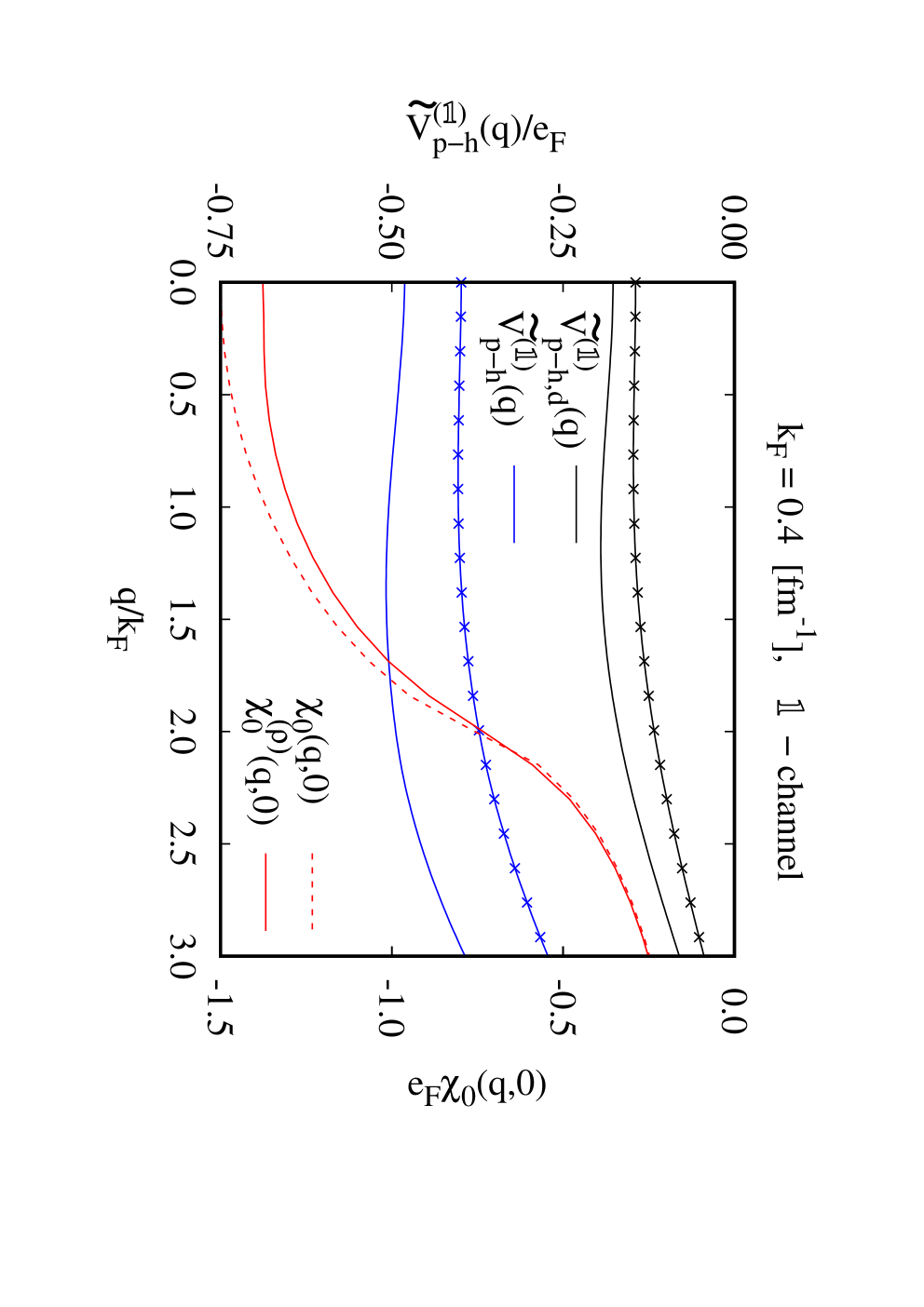
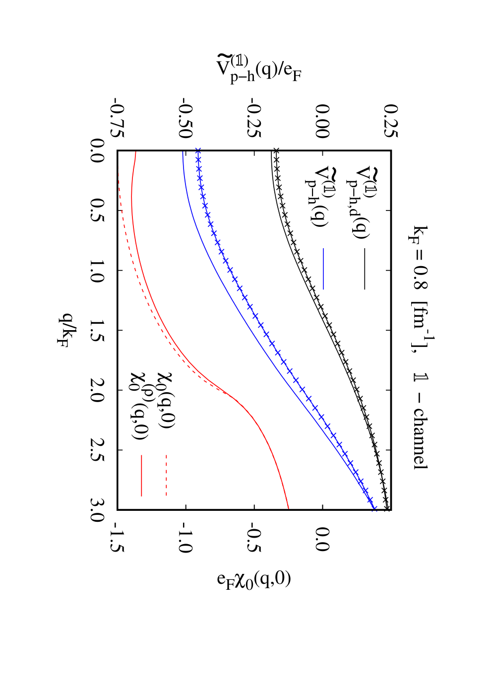
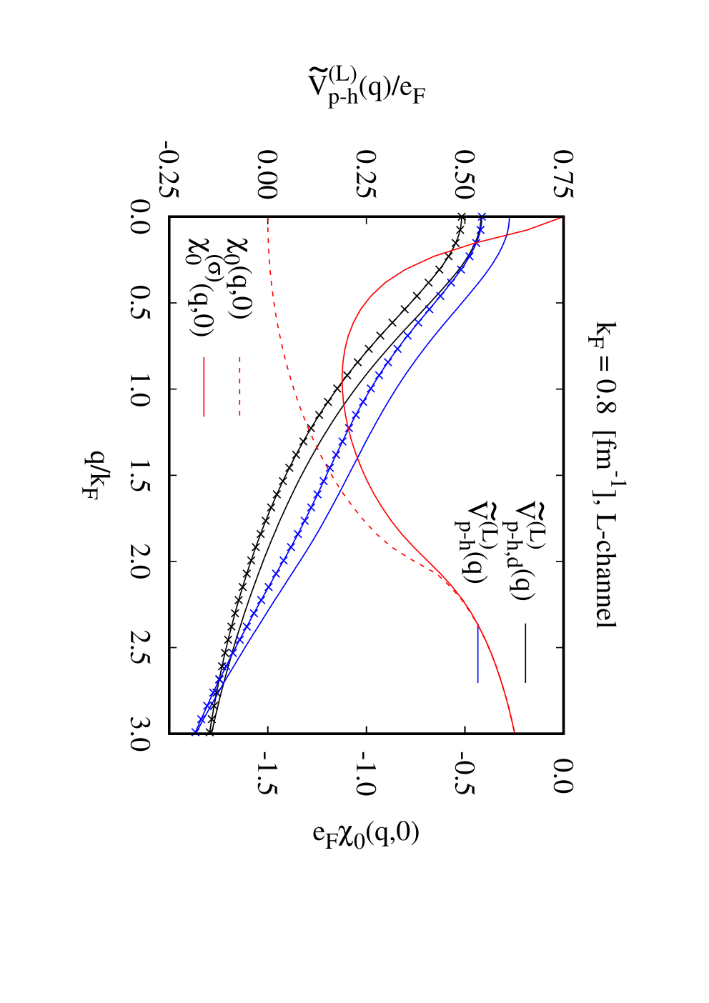
Practically all of these results look rather innocuous. As shown in our previous work Krotscheck and Wang 2020a, the inclusion of exchange diagrams is important to have a reasonably accurate relationship between the Fermi liquid parameters obtained from hydrodynamic derivatives and the long-wavelength limit of the particle-hole interaction. The “twisted chain” diagrams are the most pronounced many-body correction at low densities Krotscheck and Wang 2020b, but their effect is moderate. Considering the exponential dependence of the superfluid gap on the interaction strength, these processes can, of course, be quantitatively relevant.

The superfluid Lindhard function deviates, in the density channel, by about 10 to 20 percent from the normal system Lindhard function. The most pronounced new effect is that the superfluid Lindhard function in the spin-channel, $\chi_{0}^{(\sigma)}(q,0)$, goes to zero in the long wavelength limit. At low densities, $k_{\rm F}=0.4\,\mathrm{fm}^{-1}$, this falloff already happens at $q=k_{\rm F}$ which has the effect of suppressing the induced interaction. As expected, all corrections become smaller with increasing density. In the case of the superfluid Lindhard function, this is partly the case due to the smaller value of the gap, but evidently the correction in the spin channel is still quite visible.

Turning to the interactions that actually go into the gap equation, we show in Figs. 4 and 5 the interaction $\mathclap{\phantom{W}\mathclap{\widetilde{\mathclap{\phantom{\Gamma}\mathclap{W\,}}\phantom{\Gamma}}}}\phantom{W}(q)$ appearing in Eq. (15). A somewhat surprising, but easily understood, feature is the rather dramatic consequence of using the superfluid Lindhard function in the density channel: The fact that the long-wavelength limit $\tilde{V}_{\rm p-h}(0+)$ is of the order of $-0.5e_{\rm F}$, and that value of the Lindhard function changes by about 20 percent, can change the induced interaction by a factor of 2 which is seen in the left part of Fig. 4. This finding is consistent with the observation that the effect is smaller when non-parquet diagrams are included because the magnitude of $\tilde{V}_{\rm p-h}(0+)$ is decreased. Of course, it must be kept in mind that the agreement between the $F_{0}^{s}$ obtained from $\tilde{V}_{\rm p-h}(0+)$, see Eq. (20), and that obtained from the hydrodynamic speed of sound, Eq. (46), is only approximate Krotscheck and Wang 2020a.

The similarly significant change of the longitudinal part of the effective interaction, as shown in the right part of Fig. 4, is much more expected and comparable in both parquet and “beyond parquet” results. As we go to higher density, see Figs. 5, the effects become smaller simply due to the fact that the superfluid gap becomes smaller, but they are still quite visible.

Since we are concerned with ${}^{1}S_{0}$ pairing, we need to map the $\mathbbm{1}$, $\hat{L}$ and $\hat{T}$ channel interactions onto the $S$-wave,

$$\mathclap{\phantom{W}\mathclap{\widetilde{\mathclap{\phantom{\Gamma}\mathclap{W\,}}\phantom{\Gamma}}}}\phantom{W}^{(S)}(q)=\mathclap{\phantom{W}\mathclap{\widetilde{\mathclap{\phantom{\Gamma}\mathclap{W\,}}\phantom{\Gamma}}}}\phantom{W}^{(\mathbbm{1})}(q)-\mathclap{\phantom{W}\mathclap{\widetilde{\mathclap{\phantom{\Gamma}\mathclap{W\,}}\phantom{\Gamma}}}}\phantom{W}^{(L)}(q)-2\mathclap{\phantom{W}\mathclap{\widetilde{\mathclap{\phantom{\Gamma}\mathclap{W\,}}\phantom{\Gamma}}}}\phantom{W}^{(T)}(q)\,.$$

(47)

The interactions are shown in Fig. 6. Somewhat unexpectedly, the results show much less effect from using the superfluid Lindhard functions. The reason is found in the fact that the corrections go, in both the central and the spin channels, in the same direction and lead to an apparent partial cancellation, see Eq. (47). We could not see an argument that this cancellation is generic, but rather we consider it a coincidence.

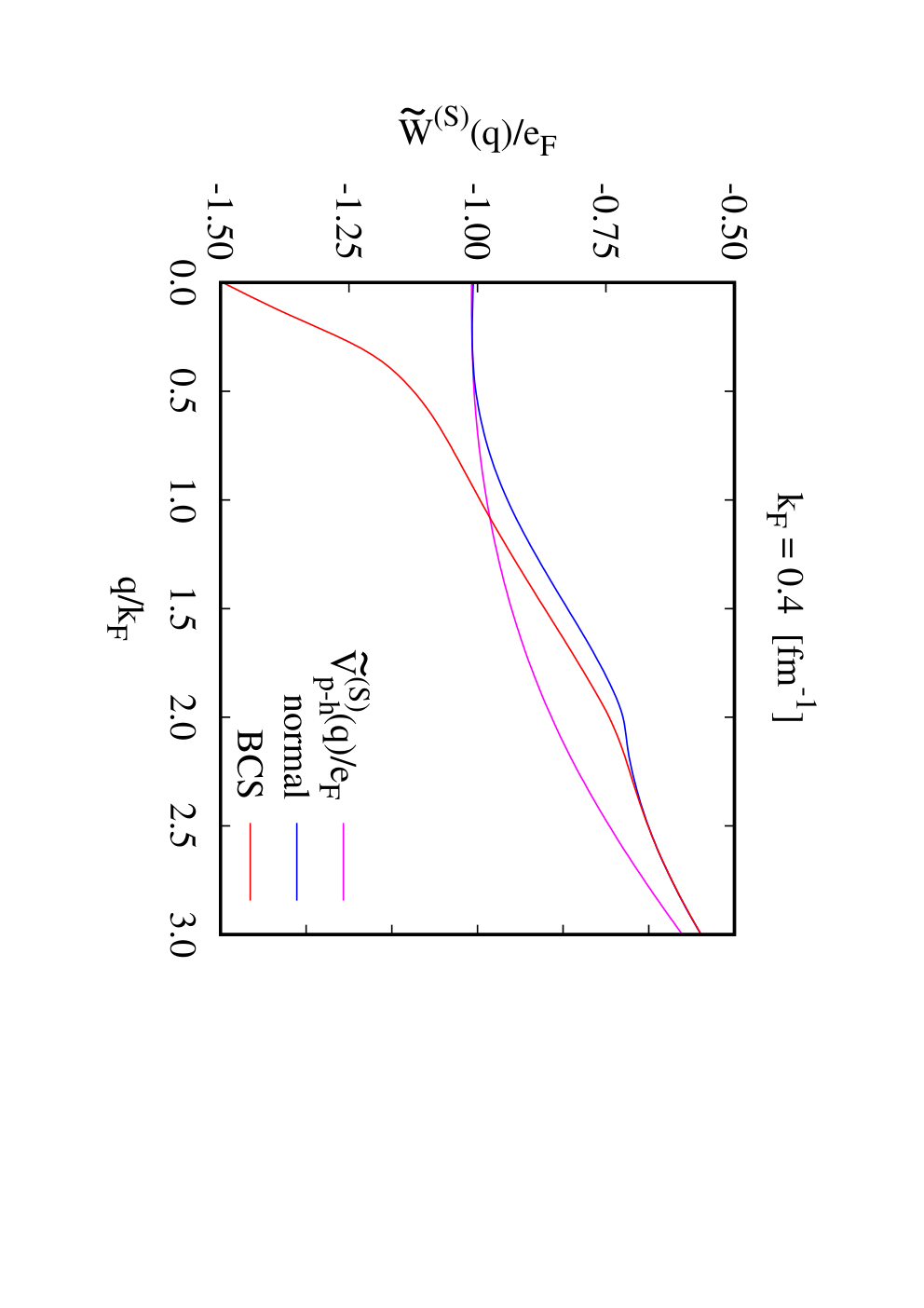
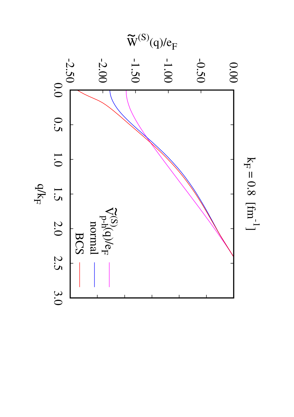
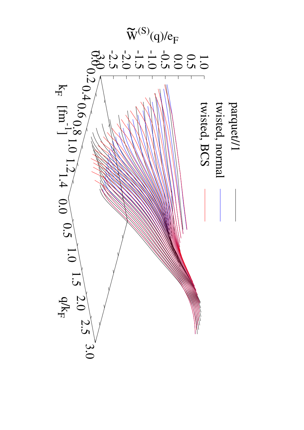
Fig. 7 gives an overall account of the density dependence of the $S$-wave pairing interaction. Generally, the inclusion of “beyond-parquet” diagrams reduces the interaction strength, the effect is most pronounced at intermediate densities. We also see clearly that the corrections from using a superfluid Lindhard function are smaller, with increasing density, at longer wavelengths which is due to the fact that the gap gets smaller.

Once the ground-state correlations and effective interactions are known, the superfluid gap function $\Delta_{{\bf k}}$ can be determined by solving the gap equation (17).

The gap equation was solved by the eigenvalue method with an adaptive mesh as outlined in the appendix of Ref. 15. We have adopted a free single-particle spectrum for $e_{{\bf k}}$ as it occurs in Eqs. (14) and (17). One could also use the actual spectrum of CBF single-particle energies Krotscheck and Clark 1979, in both the pairing interaction (14) and the denominator of Eq. (17). We have discussed and studied the effect of these modifications in previous work Fan et al. 2017, there is no reason for repetition. A recent very extensive comparison with earlier work Wambach et al. 1993; Schulze et al. 1996; Schwenk et al. 2003; Müther and Dickhoff 2005; Cao et al. 2006; Yoshida and Sagawa 2008; Gandolfi et al. 2009; Fabrocini et al. 2005; Fabrocini et al. 2008; Ding et al. 2016 is found in Ref. Pavlou et al. 2017. We can, therefore, focus in this paper on the aspect where we went beyond previous work Fan and Krotscheck 2019; Fan et al. 2017.

Our results for the superfluid gap for the two potentials are shown in Fig. 8. Evidently the difference of the gap between these two potential models is almost negligible and certainly within the accuracy of both the FHNC/parquet//1 approximation. We have above shown that specific “beyond parquet” corrections to the effective interaction should enhance the repulsion between particles in the singlet state, and Figs. 8 and 9 show exactly this effect. In fact, these contributions bring our results quite close to the quantum Monte Carlo data of Ref. Gezerlis and Carlson 2008. On the other hand, the influence of using a superfluid Lindhard function appears modest. Considering that inspection of the individual pieces of the effective interactions suggests exactly the opposite, we conclude that our specific results are circumstantial and may well be totally different for other interactions or, for example, $P$-wave pairing.

In comparison to the quantum Monte Carlo data of Ref. Gezerlis and Carlson 2008 it must, of course, be noted that our interaction model is somewhat different. We have used the full $v_{6}$ interaction, wheras Ref. Gezerlis and Carlson 2008 uses the $S$ wave part of the Argonne potential. We have tried to use that interaction too, but it turned out that the pure $S$-wave interaction leads to a spinodal instability in which case the parquet equations have no solution.