跳到论文正文
W Papers独立论文阅读器 arXiv:2010.13013 论文正文 计算阅读时间 · 0%
引用这篇论文根据当前论文元数据生成,正式投稿前建议核对。


License: arXiv.org perpetual non-exclusive license
arXiv:2010.13013v2 [cs.LG] 26 Feb 2021
 

Tractable contextual bandits beyond realizability


Sanath Kumar Krishnamurthy          Vitor Hadad          Susan Athey

Stanford University          Stanford University          Stanford University

Abstract

Tractable contextual bandit algorithms often rely on the realizability assumption – i.e., that the true expected reward model belongs to a known class, such as linear functions. In this work, we present a tractable bandit algorithm that is not sensitive to the realizability assumption and computationally reduces to solving a constrained regression problem in every epoch. When realizability does not hold, our algorithm ensures the same guarantees on regret achieved by realizability-based algorithms under realizability, up to an additive term that accounts for the misspecification error. This extra term is proportional to T times a function of the mean squared error between the best model in the class and the true model, where T is the total number of time-steps. Our work sheds light on the bias-variance trade-off for tractable contextual bandits. This trade-off is not captured by algorithms that assume realizability, since under this assumption there exists an estimator in the class that attains zero bias.

1 Introduction

Contextual bandit algorithms serve as a fundamental tool for online decision making and have been used in a wide range of settings from recommendation systems [Agarwal et al., 2016] to mobile health [Tewari and Murphy, 2017], and due to their applicability over the past couple of decades there has been an increasing amount of research in contextual bandits [Lattimore and Szepesvári, 2020]. However, the performance of many common algorithms relies on an assumption called “realizability”, which requires the analyst to possess some knowledge about the underlying data generating process – and often also relies on some luck that the process be relatively simple. When this assumption is satisfied, there exist algorithms that are statistically optimal and computationally tractable (in a sense we’ll discuss more below). However, when it is violated, the performance of these algorithms can degrade in unexpected ways. The search for tractable algorithms that do not rely on this assumption an ongoing open problem [Foster et al., 2019]. In this work, we propose an algorithm that is optimal when the “realizability” assumption is satisfied and whose behavior is accurately characterized in its absence. We will also point to directions of research that may help do away with this assumption entirely.

Our underlying setup is the general stochastic contextual bandit setting. Using potential outcome notation, observations are represented as a sequence of iid random variables (xt,rt)(x_{t},r_{t}), where xt∈𝒳x_{t}\in\mathcal{X} stands for a context in arbitrary set 𝒳\mathcal{X} and rt∈[0,1]Kr_{t}\in[0,1]^{K} is a vector of rewards, where K:=|𝒜|K:=|\mathcal{A}| is the (finite) number of actions. Upon selecting one of action at∈𝒜a_{t}\in\mathcal{A}, the algorithm observes rt​(at)r_{t}(a_{t}). Therefore, the sequence of observed data points is (xt,at,rt​(at))(x_{t},a_{t},r_{t}(a_{t})). Here tt denotes the time-step which and is also the index for the sequence of observations. This sequence has length TT, which may be known or unknown. A “policy” is a deterministic mapping from contexts to actions, representing a particular action selection strategy. Relative to the set of all policies 𝒜𝒳\mathcal{A}^{\mathcal{X}}, we define the optimal policy as π∗=arg⁡max⁡𝔼xt,rtπ∈𝒜𝒳⁡[rt​(π⁡(xt))]\pi^{*}=\arg\max_{\pi\in\mathcal{A}^{\mathcal{X}}}\mathop{\mathbb{E}}_{x_{t},r_{t}}[r_{t}(\pi(x_{t}))], where the expectation is taken over contexts and rewards.11 1 Uniqueness of the optimal policy is not important for our results. A “reward model” or “outcome model” is a function that (potentially inaccurately) represents the conditional expectation of potential outcomes given action and context. Reward models will often be represented as f⁡(x,a)f(x,a). We say that a reward model “induces a policy π\pi” if π⁡(x)∈arg⁡maxa⁡f⁡(x,a)\pi(x)\in\arg\max_{a}f(x,a) for every xx.

The goal of bandit algorithms is to find a sequence of actions that maximizes the sum of rewards observed during the experiment or, equivalently, to minimize cumulative regret, defined as the difference between the reward that was observed and that that would have been observed under the optimal policy,

RT:=∑t=1Trt​(π∗​(xt))−rt​(at).\displaystyle R_{T}:=\sum_{t=1}^{T}r_{t}(\pi^{*}(x_{t}))-r_{t}(a_{t}). (1)

The statistical performance of different algorithms is characterized by the rate at which (1) grows with the length of the experiment TT.

Contextual bandit algorithms can often be categorized into three groups, depending on what is assumed about the underlying data-generating process. The first group of algorithms are the “agnostic” algorithms. These algorithms make no assumptions about the reward model, and they learn the best policy in some fixed class Π⊆𝒜𝒳\Pi\subseteq\mathcal{A}^{\mathcal{X}} while balancing the exploration-exploitation trade-off. To do this, these algorithms [Beygelzimer et al., 2011, Dudik et al., 2011, Agarwal et al., 2014] need to construct a distribution over the policies Π\Pi in every epoch. Constructing this distribution is computationally challenging, and hence this approach is colloquially referred to as the “Monster” [Langford, 2014]. We now focus on the results in [Agarwal et al., 2014] because computationally and statistically, they provide the state of the art agnostic algorithms. When Π\Pi is a finite class, [Agarwal et al., 2014] present an algorithm called ILTCB that constructs a distribution with support size of 𝒪⁡(log⁡|Π|)\mathcal{O}(\log|\Pi|) and the regret 22 2 Note that while this notion of regret compares against the best policy in Π\Pi, the notion of regret used in this paper compares against the true optimal policy π∗\pi^{*}. against the best policy in Π\Pi scales at the rate 𝒪~​(K​T​log⁡|Π|)\tilde{\mathcal{O}}(KT\log|\Pi|). Each policy in the support of this distribution can be computed by solving the following cost-sensitive classification problem:

arg⁡max⁡∑s=1tπ∈Π⁡r^s​(π⁡(xs)),\displaystyle\arg\max_{\pi\in\Pi}\sum_{s=1}^{t}\hat{r}_{s}(\pi(x_{s})), (2)

where (xs,r^s)(x_{s},\hat{r}_{s}) is some sequence in 𝒳×[0,1]K\mathcal{X}\times[0,1]^{K}. When Π\Pi is large, the support of the distribution needed to be computed in every epoch of ILTCB may be large and hence would still be impractical to implement. To overcome this limitation, [Agarwal et al., 2014] propose a heuristic called Online Cover (with parameter ll) that computes a distribution over polices using the same approach as ILTCB but stops increasing the support of this distribution after computing some fixed number of policies ll for the support. To the best of our knowledge there aren’t any theoretical guarantees for Online Cover. Further, finding an exact solutions to (2) is generally intractable, so implementations of Online Cover use heuristics to solve this optimization problem.

The second group of algorithms requires knowledge about some set of functions ℱ\mathcal{F} that is assumed to include the true reward model. That is, that there exists a function f∗∈ℱf^{*}\in\mathcal{F} such that f∗​(x,a)=𝔼xt,rt[rt​(a)|xt=x]f^{*}(x,a)=\mathop{\mathbb{E}}_{x_{t},r_{t}}[r_{t}(a)|x_{t}=x] for all contexts and actions. This assumption is called “realizability”, and it often allows for algorithms that computationally tractable and typically easier to implement. Computationally, algorithms in this category rely on being able to solve the regression problem

f^t=arg⁡min⁡∑s=1t−1f∈ℱ⁡(f⁡(xs,as)−rs​(as))2,\displaystyle\hat{f}_{t}=\arg\min_{f\in\mathcal{F}}\sum_{s=1}^{t-1}(f(x_{s},a_{s})-r_{s}(a_{s}))^{2}, (3)

or a weighted version of it, either online or offline. A routine that solves (3) is called “regression oracle”. This class includes algorithms built on upper confidence bounds [Li et al., 2010, Abbasi-Yadkori et al., 2011, Foster et al., 2018] or Thompson sampling [Agrawal and Goyal, 2013, Russo et al., 2018], and algorithms built on simple probabilistic selection strategies [Abe and Long, 1999, Foster and Rakhlin, 2020, Simchi-Levi and Xu, 2020]. Regret rates for this class of algorithms are related to the complexity class of the outcome model ℱ\mathcal{F}, and under realizability optimal algorithms attain a rate of 𝒪~​(T​K​log⁡|ℱ|)\tilde{\mathcal{O}}(\sqrt{TK\log|\mathcal{F}|}) for finite classes ℱ\mathcal{F} (similar results are available for more general classes). In particular, the FALCON algorithm of [Simchi-Levi and Xu, 2020] will serve as the basis of our method attains this statistically optimal rate (so long as realizability holds) and is computationally tractable, in that the algorithm only needs to solve the problem (3) a small (at most logarithmic) number of times during the experiment.

Refer to caption
Figure 1: Example. Data-generating process (left) and its best approximation in the class of linear functions (right). The induced policies are the same.
Refer to caption
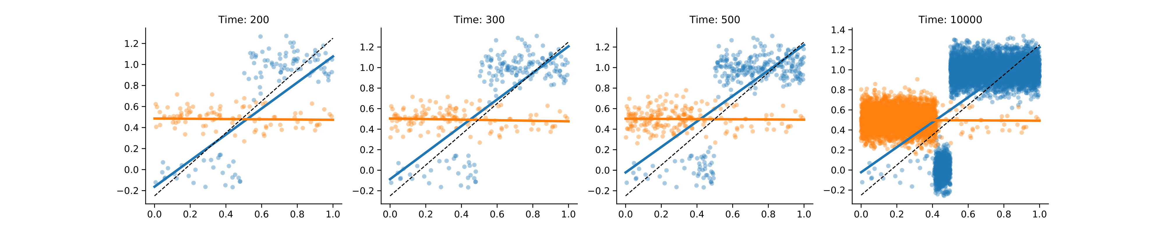
Figure 2: Evolution of model estimates for the UCB example. Although the model is initially correct, the distribution shift caused by the assignment mechanism ends up biasing reward estimates over time. Best linear approximation in black, dotted line. In our proposed algorithm, the blue and black lines are kept appropriately close, preventing this phenomenon.

A third set of bandit algorithms that does not fall neatly into any of the two categories above are algorithms that allow for a non-parametric model class. For example, in [Rigollet and Zeevi, 2010], [Perchet et al., 2013] the reward model is assumed to be Hölder continuous but non-differentiable, and in [Hu et al., 2020], [Gur et al., 2019] it satisfies a Hölder smoothness assumption. The main characteristic of this class of algorithms is that they partition the covariate space into hypercubes of appropriate size and run multi-armed bandit algorithms within each cube. Depending on the smoothness of the reward model, there can be some information sharing across cubes that induces correlation across assignments in adjacent hypercubes and decreases regret. Although this is a very interesting direction of research, the structure of these algorithms forces the running time to exponentially depend on the context dimension, making them computationally intractable and hard to implement for most real life problems. Hence, for the rest of the paper, we will focus on the first two classes of algorithms.

1.1 The problem with realizability

As we have mentioned before, realizability is an extremely convenient and pervasive assumption in many tractable contextual bandit algorithms, but it is nevertheless very strong. In this section, we attempt to shed light on some issues that may arise in its absence.

To fix ideas, start from the following illustration. There are two actions and a single context is distributed uniformly on the unit interval. However, unbeknownst to the researcher, the conditional average rewards for each arm are a step function f1∗(xt):=𝕀{xt>0.5}f_{1}^{*}(x_{t}):=\mathbb{I}\{x_{t}>0.5\} and a constant f2∗​(xt)≡0.5f_{2}^{*}(x_{t})\equiv 0.5 (Figure 1). Rewards are observed with error ϵt∼𝒩⁡(0,.01)\epsilon_{t}\sim\mathcal{N}(0,.01). The researcher erroneously assumes that both can be realized in the class ℱ\mathcal{F} of linear functions. Fortunately, in this example the best linear approximation (f^1∗,f^2∗)(\hat{f}_{1}^{*},\hat{f}_{2}^{*}) induces a good policy. In fact, it coincides with the one the researcher would obtain if they had knowledge about the true function class – i.e., the policy induced by the best linear approximation π^∗\hat{\pi}^{*} defined by π^​(x)=1\hat{\pi}(x)=1 if x>0.5x>0.5 and π^​(x)=2\hat{\pi}(x)=2 otherwise actually coincides with the policy induces by the true model π∗​(x):=arg⁡maxa​f∗​(x,a)\pi^{*}(x):=\arg\max_{a}f^{*}(x,a). Therefore, if the sequence of fitted models (f^1,t,f^2,t)(\hat{f}_{1,t},\hat{f}_{2,t}) converges to the best linear approximation (f^1,t∗,f^2,t∗)(\hat{f}_{1,t}^{*},\hat{f}_{2,t}^{*}), regret should decay to zero asymptotically. However, as we will see next, this convergence may not happen.

Let us assume that the researcher collects data via LinUCB [Li et al., 2010], with model updates in batches of 100 observations. Figure 2 shows the evolution of the estimated models (f^1,t,f^2,t)(\hat{f}_{1,t},\hat{f}_{2,t}) over time for a single simulation. After about a few hundred observations, the estimated model approximates the best linear approximation well and regret is small since the induced policy is nearly optimal. However, by continuing to assign treatments following this policy (plus some negligible exploration), the distribution of observations changes, which pushes the model away from the best linear approximation. In turn, this causes per-period regret to increase over time, as we show on Figure 3.

Refer to caption
Figure 3: Evolution of per-period regret for the UCB example described in the text. Regret initially decreases because the estimated models (f^1,t,f^2,t)(\hat{f}_{1,t},\hat{f}_{2,t}) are close to the best linear approximations (f^1∗,f^2∗)(\hat{f}^{*}_{1},\hat{f}^{*}_{2}), which in this example induces a good policy. However, as we gather more data that was collected with an exploitation objective, the estimated model diverges and the performance of the algorithm degrades. (Average across 100 simulations.)

The previous example demonstrates that in the absence of realizability the dynamics of adaptive data collection can lead the algorithm to learn a policy that is suboptimal relative to the one that it would have learned under non-adaptive data collection. As an extreme thought example, one may also consider a situation in which actions are assigned via the optimal policy π∗\pi^{*}. If we were to fit a linear model using exclusively this data, we would estimate that f^1≡1\hat{f}_{1}\equiv 1 and f^2≡0.5\hat{f}_{2}\equiv 0.5, which would in turn induce the policy π⁡(x)≡1\pi(x)\equiv 1 – a policy that always assigns arm 11 everywhere and therefore clearly suboptimal. In fact, more can be said. We can construct examples where even when the approximation error bb is arbitrarily small, given data from the optimal policy, the confidence intervals used by LinUCB would tightly concentrate around a high regret policy, showing that the confidence intervals used by LinUCB are extremely sensitive to the realizability assumption (See Appendix E).

To prevent this phenomenon, in the next section we consider an algorithm that constraints the estimate of the outcome model f^\hat{f} to be close to f^∗\hat{f}^{*}. This also allows us to derive upper bounds on regret in terms of the deviation of the best in-class model f^∗\hat{f}^{*} from the true model f∗f^{*}. This characterization is important as it allows us to take into account regret incurred due to model misspecification – a cost that often assumed away under realizability.

1.2 Related work on misspecification

As we have discussed above, bandit algorithms relying on regression oracles are computationally tractable, and when their model is well-specified they often exhibit attractive statistical properties. More recently, there has been interest in developing algorithms that are robust to misspecification. These works differ in how they define and measure misspecification, and how their regret bound degrade as the level of misspecification increases.

[Neu and Olkhovskaya, 2020, Zanette et al., 2020] assume that the absolute deviation between the true reward function and its best linear approximation is at most ϵ\epsilon uniformly across contexts and actions. Under this assumption, they develop bandit algorithms whose regret overhead due to misspecification is bounded in terms of this measure of misspecification ϵ\epsilon. Under the same measure of misspecification, [Foster and Rakhlin, 2020] provide similar results that hold for any class of models that have an online regression oracle.

This type of uniform bound on model misspecification can be arbitrarily large even in relatively benign examples (see Appendix E). Concurrent work of [Foster et al., 2020] use a different measure of misspecification that allows them to derive tighter regret bounds while relying on online regression oracles. Their measure of misspecification turns out to be very similar to the one we use in this work, however we rely on constrained offline regression oracles instead. Moreover, [Foster et al., 2020] also adapt to unknown misspecification by relying on master algorithms (see Section 3).

[Lattimore et al., 2020] and [Ghosh et al., 2017] also study the related problem of misspecified non-contextual linear bandits.

2 Main results

We propose an algorithm that we call Epsilon-FALCON, which is a modification of the “FAst Least-squares-regression-oracle CONtextual bandits”, or FALCON algorithm described in [Simchi-Levi and Xu, 2020]. The main departure from FALCON is that although we do posit some “tentative” set ℱ\mathcal{F} that could contain the true outcome model, our regret guarantees do not depend on this assumption being satisfied. For simplicity of exposition we will initially assume that ℱ\mathcal{F} is a convex subset of a dd-dimensional linear space 33 3 Consider the class of estimators ℱ\mathcal{F} where linear functions estimate rewards for each arm using a total of dd parameters. Note that this is a special case of requiring ℱ\mathcal{F} to be a convex subset of a dd-dimensional linear space. Hence, the guarantees in Theorem 1 hold for stochastic linear bandits., but our results can be extended to more complex classes as we show later.

We will need some additional notation. Let f∗f^{*} represent the true outcome model, i.e., f∗​(x,a)=𝔼xt,rt[rt​(a)|xt=x]f^{*}(x,a)=\mathop{\mathbb{E}}_{x_{t},r_{t}}[r_{t}(a)|x_{t}=x] for all xx and aa. Moreover, let f^∗\hat{f}^{*} denote the best in-class approximation to the true outcome model when data is collected non-adaptively, or

f^∗:=arg⁡minf∈ℱ​𝔼x∼D𝒳𝔼a∼Unif​(𝒜)[(f⁡(x,a)−f∗​(x,a))2],\hat{f}^{*}:=\arg\min_{f\in\mathcal{F}}\mathop{\mathbb{E}}_{x\sim D_{\mathcal{X}}}\mathop{\mathbb{E}}_{a\sim\text{Unif}(\mathcal{A})}[(f(x,a)-f^{*}(x,a))^{2}], (4)

where D𝒳D_{\mathcal{X}} is the distribution of contexts, and Unif​(𝒜)\text{Unif}(\mathcal{A}) is a probability distribution that assigns equal probability to every arm. The approximation error between these two functions is denoted as

b:=𝔼x∼D𝒳𝔼a∼Unif​(𝒜)[(f^∗​(x,a)−f∗​(x,a))2].\displaystyle b:=\mathop{\mathbb{E}}_{x\sim D_{\mathcal{X}}}\mathop{\mathbb{E}}_{a\sim\text{Unif}(\mathcal{A})}[(\hat{f}^{*}(x,a)-f^{*}(x,a))^{2}]. (5)

Naturally, the approximation error (5) will be zero when realizability holds. And when it doesn’t hold, we will show that the algorithm will incur some regret whose upper bound increases with the approximation error. This is what allows us to accurately characterize the cost that we pay when we ℱ\mathcal{F} is misspecified (i.e., f∗∉ℱf^{*}\not\in\mathcal{F}).

Algorithm:

Epsilon-FALCON is implemented in increasing epochs (batches) that are indexed by mm. Each epoch mm begins at period τm−1\tau_{m-1}, we set epoch schedule so that τ0=0\tau_{0}=0, τ1≥4\tau_{1}\geq 4, and τm+1=2​τm\tau_{m+1}=2\tau_{m} for any epoch m≥1m\geq 1. Every epoch mm starts out with an estimated reward model f^m\hat{f}_{m} obtained at the end of the last batch, with f^1≡0\hat{f}_{1}\equiv 0. For a fraction ϵ\epsilon of each epoch, called the “passive” phase, Epsilon-FALCON draws actions uniformly at random. For the remaining 1−ϵ1-\epsilon fraction of the epoch, in what we call the ‘‘active’’ phase, it acts as a modified version of FALCON.44 4 More precisely, it acts as a modified version of the FALCON+ algorithm in the same paper, but the distinction is minor enough that we will ignore it for the purposes of naming our method.

Our action selection mechanism is the same as FALCON’s, so let’s briefly review it. At each epoch mm, given the current reward model estimate f^m\hat{f}_{m} and a scaling parameter γm>0\gamma_{m}>0, actions are drawn from the probability distribution described by the following “action selection kernel”,

pm​(a|x):={1K+γm​(f^m​(x,a^)−f^m​(x,a))for ​a≠a^1−∑a′≠a^p⁡(a′|x)for ​a=a^.\displaystyle p_{m}(a|x):=\begin{cases}\frac{1}{K+\gamma_{m}\left(\hat{f}_{m}(x,\hat{a})-\hat{f}_{m}(x,a)\right)}&\text{for }a\neq\hat{a}\\ 1-\sum_{a^{\prime}\neq\hat{a}}p(a^{\prime}|x)&\text{for }a=\hat{a}.\end{cases} (6)

where a^=maxa⁡f^m​(a,x)\hat{a}=\max_{a}\hat{f}_{m}(a,x) is the best predicted action. The assignment rule (6) ensures that actions that are predicted to be good according to the current model estimate f^m\hat{f}_{m} are given higher probability. The scaling parameter, set to γm≃K⁡(τm−1−τm−2)/(d​ln⁡(m/δ))\gamma_{m}\simeq\sqrt{K(\tau_{m-1}-\tau_{m-2})/(d\ln(m/\delta))} with initial values γ1=1\gamma_{1}=1, control the degree of exploration during the active phase, with higher values of γm\gamma_{m} indicating less exploration. We may sometimes refer to γm\gamma_{m} and ϵ\epsilon as the active and passive exploration parameters respectively.

The main difference between our method and FALCON is in how we estimate the outcome model f^m+1\hat{f}_{m+1} from data collected in the previous epoch mm. The original algorithm simply uses the estimator that minimizes empirical risk on data collected in the previous time-steps, but as we saw in the example in Section 1.1, when realizability fails the sequence of estimators f^m\hat{f}_{m} may not converge to f^∗\hat{f}^{*}. This is due to the fact that the empirical risk minimizer when data is collected adaptively may be very different from the one attained when data is collected non-adaptively, and its performance may not be well understood (See Figure 4). In order to ensure that our estimates converge to f^∗\hat{f}^{*}, our algorithm uses a “constrained regression oracle” that ensures that the estimated model is always close to the best approximation f^∗\hat{f}^{*}. Let’s see how this is done.

Denote the data collected using the passive and active phases of the epoch mm by Sm′S_{m}^{\prime} and SmS_{m} respectively. Moreover, let ℱm′\mathcal{F}^{\prime}_{m} denote the subset of functions f∈ℱf\in\mathcal{F} for which the following constraint in satisfied,

∑(x,a,r⁡(a))∈Sm′(f⁡(x,a)−r⁡(a))2≤αm+C1​d​ln⁡(12​m2/δ)\sum_{(x,a,r(a))\in S_{m}^{\prime}}(f(x,a)-r(a))^{2}\leq\alpha_{m}+C_{1}d\ln(12m^{2}/\delta) (7)

where αm:=min⁡∑(x,a,r⁡(a))∈Sm′g∈ℱ⁡(g⁡(x,a)−r⁡(a))2\alpha_{m}:=\min_{g\in\mathcal{F}}\sum_{(x,a,r(a))\in S_{m}^{\prime}}(g(x,a)-r(a))^{2} is the sum of squared residuals in the model fitted on the data collected in the “passive” phase, and C1C_{1} is a constant chosen appropriately to ensure that f^∗\hat{f}^{*} also lies in ℱ′\mathcal{F}^{\prime} with probability at least 1−δ/(12​m2)1-\delta/(12m^{2}). 55 5 We pin down the value of this constant in the Appendix

The estimated model f^m+1\hat{f}_{m+1} will be constrained to lie in this set. More specifically, it is the output of the following constrained regression problem:

minf∈ℱ\displaystyle\min_{f\in\mathcal{F}} ∑(x,a,r⁡(a))∈Sm(f⁡(x,a)−r⁡(a))2\displaystyle\sum_{(x,a,r(a))\in S_{m}}(f(x,a)-r(a))^{2} (8)
s.t.\displaystyle\textrm{s.t.} f∈ℱm′.\displaystyle f\in\mathcal{F}^{\prime}_{m}.

The intuition, again, is that since f^m+1∈ℱm′\hat{f}_{m+1}\in\mathcal{F}^{\prime}_{m} by construction, and since f^∗∈ℱm′\hat{f}^{*}\in\mathcal{F}^{\prime}_{m} with high probability, the two will likely remain close. And since ℱm′\mathcal{F}^{\prime}_{m} shrinks over time, f^m+1\hat{f}_{m+1} must ultimately converge to f^∗\hat{f}^{*}. Therefore, the convergence issues we saw in our example in Section 1.1 cannot happen. This is what allows us to derive regret guarantees even when realizability fails (see Figure 4 for an intuitive illustration). The full description and the pseudocode for the general algorithm can be found in the Appendix (Algorithm 1). 66 6 Except for the choice of γm\gamma_{m} and the RHS of the constraint Equation 7, the algorithm for general ℱ\mathcal{F} is the same as the description in this section.

Refer to caption
Figure 4: Intuition for our method. Left: the function f^∗\hat{f}^{*} is the best in-class approximation to f∗f^{*} under non-adaptive data collection. Middle: under a different distribution, the best in-class approximation (starred) may lie very far away from f^∗\hat{f}^{*}, and there are no guarantees on its performance. Right: in our method, we construct a shrinking sequence of sets ℱm′\mathcal{F}^{\prime}_{m} that contain f^∗\hat{f}^{*} with high probability, and ensure that our model estimates lie in this set.

Computational tractability of the constrained regression problem:

Note that Epsilon-FALCON is very easy to implement given a constrained regression oracle. Hence, for the computational tractability of Epsilon-FALCON, it is sufficient to argue that the constrained regression problem is computationally tractable. When ℱ\mathcal{F} is the class of linear reward models, then clearly the constrained regression problem is a convex and can be solved efficiently. In general, when ℱ\mathcal{F} is any convex class, we show that the constrained regression problem can be solved efficiently with a weighted regression oracle (see Appendix D). Hence we can use any of the many existing algorithms for weighted regression as a subroutine to solve the constrained regression problem. While this is one approach to solve the constrained regression problem, in practice directly solving the constrained regression problem may be faster.

Theorem 1 provides a high probability regret guarantee for Epsilon-FALCON when ℱ\mathcal{F} is a convex subset of some dd-dimensional linear space.

Theorem 1 (Linear case).

Suppose ℱ\mathcal{F} is a convex subset of a dd-dimensional linear space. With probability at least 1−δ1-\delta, Epsilon-FALCON with passive exploration parameter ϵ>0\epsilon>0 attains the following regret guarantee:

RT≤𝒪⁡(K​T​d​ln⁡(ln⁡(T)δ)+K​T​bϵ+ϵ​T).\displaystyle R_{T}\leq\mathcal{O}\left(\sqrt{KTd\ln\Big(\frac{\ln(T)}{\delta}\Big)}+KT\sqrt{\frac{b}{\sqrt{\epsilon}}}+\epsilon T\right). (9)

The guarantees in (9) consist of three terms. The first term is the regret due to the complexity of the class ℱ\mathcal{F}, and is the bound guaranteed by realizability based algorithms like FALCON under realizability. The second term can be interpreted as the “cost of misspecification”, this term depends on the approximation error bb and the passive exploration parameter ϵ\epsilon. Finally, the third term is the regret incurred in the passive phase and depends only on the passive exploration parameter ϵ\epsilon.

At first glance, the result in (9) may look rather weak due to the linear dependence in the horizon TT. However, we contend that any algorithm that that works with a restricted class of policies or reward models, including agnostic algorithms like ILTCB [Agarwal et al., 2014], will incur some linear regret if these restrictions are violated. In Theorem 1 we simply make this issue explicit, as one of our goals is to accurately characterize the bias-variance trade-off in our problem. Our results show that, if the practitioner is willing to spend ϵ​T\epsilon T regret in the passive phase, then in the active phase excess regret due to misspecification will be 𝒪⁡(K​T​b/ϵ)\smash{\mathcal{O}(KT\sqrt{b/\sqrt{\epsilon}})}. On the other hand, realizability based approaches do not have any guarantees under general misspecification.

As a thought experiment, suppose we knew the approximation error bb or could make an educated guess about it. In that case we could choose ϵ\epsilon as a function of bb so as to optimize (9) and obtain the next result.

Corollary 1 (Linear case with known bb).

In the setting of Theorem 1, if the passive exploration parameter is set to ϵ=c​K4/5​b2/5\epsilon=cK^{4/5}b^{2/5} for some constant c>0c>0, we have the following bound:

RT≤𝒪⁡(K​T​d​ln⁡(ln⁡(T)δ)+K4/5​b2/5​T).\displaystyle R_{T}\leq\mathcal{O}\left(\sqrt{KTd\ln\Big(\frac{\ln(T)}{\delta}\Big)}+K^{4/5}b^{2/5}T\right). (10)

This result is interesting because it tells us that if we were able to tune the passive exploration parameter optimally, we get improved regret rates that only depend on the complexity of ℱ\mathcal{F} and the approximation error bb, thus achieving a bias-variance trade-off over the entire horizon TT. This suggests that tuning ϵ\epsilon by estimating bb may be a promising direction for future work to get algorithms with better regret guarantees.

Understanding the constrained regression problem:

Having explained the overall algorithm, let’s now understand the constrained regression problem in a bit more detail, so the reader will be able to follow the proof steps in the Appendix.

At the end of epoch mm, we have the two kinds of data, that is the data from the passive phase of the epoch and the data from the active phase of the epoch. The data from the passive phase is used to construct ℱm′\mathcal{F}^{\prime}_{m}, and contains the best in-class approximation of the true outcome model f^∗\hat{f}^{*} with high probability (see Lemma 7). The data from the active phase is used to select a “good” estimate within ℱm′\mathcal{F}^{\prime}_{m} which in turn induces a “good” action selection kernel. A good action selection kernel has low regret, and ensures that the data generated by this kernel can be used to construct “good” estimates in the next epoch. In terms of exploration, there is a trade-off between these two properties as more exploration helps you generate “good” data but incurs higher regret. In terms of estimates, both these properties are related because good estimates come from good data. For simplicity let us focus on arguing that the action selections kernels we estimate generate “good” data and believe that the active exploration parameter γm\gamma_{m} is set optimally. In particular, we say the action selection kernel generates “good” data if the reward of the policy induced by f^∗\hat{f}^{*} can be estimated using the data generated by this kernel. Note that this is trivially ensured when actions are selected uniformly at random, as we did in the first epoch. In later epochs, as the kernel gets less explorative (γm\gamma_{m} increases), to ensure this we need the estimator (f^m+1\hat{f}_{m+1}) that induces this action selection kernel to be close to the best in-class model (f^∗\hat{f}^{*}). More mathematically, as shown in Lemma 9, we need the root mean squared difference between f^m+1\hat{f}_{m+1} and f^∗\hat{f}^{*} to shrink at the same rate as γm\gamma_{m} increases. This property is guaranteed by the fact that both f^m+1\hat{f}_{m+1} and f^∗\hat{f}^{*} lie in ℱm′\mathcal{F}^{\prime}_{m} with high probability, and by the fact that ℱm′\mathcal{F}^{\prime}_{m} is sufficiently small as we have collected enough data in the passive phase to ensure this (see Lemma 7). Additionally, this property helps us ensure that our action selection kernels pmp_{m} are stable over time, in the sense that if the reward of a policy could be estimated from the data generated by pm+1p_{m+1} (in expectation) then the reward of this policy could also be estimated by the data generated by pmp_{m} (in expectation), see Lemma 10 for a more formal statement. In other words, the set of policies that we implicitly consider do not erratically change over time and only decrease.

General classes of outcome models:

Although for concreteness we have explained our results when ℱ\mathcal{F} is a convex subset of a dd-dimensional linear space, Theorem 1 readily extends to more general classes of functions. In particular we can extend Theorem 1 whenever ℱ\mathcal{F} is a convex and satisfies 1. In terms of the algorithm, except for the choice of γm\gamma_{m} and the RHS of the constraint Equation 7, Epsilon-FALCON for general ℱ\mathcal{F} is the same as the description in this section. See Algorithm 1 in the Appendix for more details. Stating 1 can get cumbersome quickly, here we state an informal version of this assumption, followed by Theorem 2, and applications of this Theorem to various convex classes ℱ\mathcal{F}. In what follows comp​(ℱ)\textbf{comp}(\mathcal{F}) will denote an appropriate measure of complexity, like VC subgraph dimension or entropy.

Main Assumption:

We now state an informal version of 1. Let nn denote the number of data points collected from some distribution. Suppose we have ρ∈(0,1]\rho\in(0,1], ρ′∈[0,∞)\rho^{\prime}\in[0,\infty), and C>0C>0. Further suppose for any convex subset ℱ′\mathcal{F}^{\prime} of ℱ\mathcal{F} and ζ∈(0,1/2)\zeta\in(0,1/2), with probability 1−ζ1-\zeta, for any η≥C​lnρ′⁡(n)​ln⁡(1/ζ)​comp​(ℱ)/nρ\eta\geq C\ln^{\rho^{\prime}}(n)\ln(1/\zeta)\textbf{comp}(\mathcal{F})/n^{\rho}, the empirical and true risks of any estimators in ℱ′\mathcal{F}^{\prime} are “close” in the following sense:

  • •

    If the population risk of any estimator in ℱ′\mathcal{F}^{\prime} is smaller than η\eta, then its empirical risk is not larger than 3​η/23\eta/2.

  • •

    If the empirical risk of any estimator in ℱ′\mathcal{F}^{\prime} is smaller than η\eta, then its population risk is not larger than 2​η2\eta.

Theorem 2 (Main result).

Suppose ℱ\mathcal{F} is a convex set and suppose 1 holds. Then with probability at least 1−δ1-\delta, Epsilon-FALCON with passive exploration parameter ϵ>0\epsilon>0 attains the following regret guarantee:

RT≤𝒪⁡(CLOSEK​T2−ρ​lnρ′⁡(T)​ln⁡(ln⁡(T)δ)​comp​(ℱ)OPEN+K​T​bϵρ+ϵ​T).\displaystyle\begin{split}R_{T}\leq\mathcal{O}\Bigg(&\sqrt{KT^{2-\rho}\ln^{\rho^{\prime}}(T)\ln(\frac{\ln(T)}{\delta})\textbf{comp}(\mathcal{F})}\\ &\;\;+KT\sqrt{\frac{b}{\sqrt{\epsilon^{\rho}}}}+\epsilon T\Bigg).\end{split} (11)

In Appendix C, we provide convenient Lemmas to prove 1 for various convex classes ℱ\mathcal{F}. These Lemmas directly follow from results in [Koltchinskii, 2011]. In fact, Theorem 1 is implied by Theorem 2 and results stated in Appendix C. We now go over similar results that follow from Theorem 2 and Appendix C.

Example 1: Suppose ℱ\mathcal{F} is convex and has VC-subgraph dimension VV. Then with probability 1−δ1-\delta, Epsilon-FALCON guarantees the following bound on the regret RTR_{T}:

𝒪⁡(K​T​V​ln⁡(TV)​ln⁡(ln⁡(T)δ)+K​T​bϵ+ϵ​T).\mathcal{O}\Bigg(\sqrt{KTV\ln\bigg(\frac{T}{V}\bigg)\ln\bigg(\frac{\ln(T)}{\delta}\bigg)}+KT\sqrt{\frac{b}{\sqrt{\epsilon}}}+\epsilon T\Bigg).

Example 2: Suppose ℱ\mathcal{F} is a convex hull of class with VC-subgraph dimension VV. Then with probability 1−δ1-\delta, Epsilon-FALCON guarantees the following bound on the regret RTR_{T}:

𝒪⁡(K​T2+3​V2+2​V​V2+V2+2​V​ln⁡(ln⁡(T)δ)+K​T​bϵ+ϵ​T).\mathcal{O}\Bigg(\sqrt{KT^{\frac{2+3V}{2+2V}}V^{\frac{2+V}{2+2V}}\ln\bigg(\frac{\ln(T)}{\delta}\bigg)}+KT\sqrt{\frac{b}{\sqrt{\epsilon}}}+\epsilon T\Bigg).

Example 3: Suppose for some ρ∈(0,1)\rho\in(0,1), the empirical entropy is bounded by 𝒪⁡(ϵ−2​ρ)\mathcal{O}(\epsilon^{-2\rho}) for all empirical distributions. Then with probability 1−δ1-\delta, Epsilon-FALCON guarantees the following bound on the regret RTR_{T}:

𝒪⁡(K​T1+2​ρ1+ρ​ln⁡(ln⁡(T)δ)+K​T​bϵ1/(1+ρ)+ϵ​T).\mathcal{O}\Bigg(\sqrt{KT^{\frac{1+2\rho}{1+\rho}}\ln\bigg(\frac{\ln(T)}{\delta}\bigg)}+KT\sqrt{\frac{b}{\sqrt{\epsilon^{1/(1+\rho)}}}}+\epsilon T\Bigg).

3 Discussion

This paper’s contribution is twofold. First, to illustrate how algorithms that rely on realizability may incur unexpected regret when this assumption is violated. We saw in Section 1.1 that one can construct examples where regret is large even in relatively benign settings. Second, to propose a flexible family of computationally tractable algorithm that are less sensitive to realizability. Our analysis in Section 2 characterizes the behavior of regret under misspecification and gives us insight into the bias-variance trade-off in contextual bandits.

In terms of algorithm design, our proposed algorithm Epsilon-FALCON inherits the computational elegance of realizability based approaches like FALCON. In particular, a single estimator gives you an implicit distribution over policies via the action selection kernel and bypasses the need to explicitly construct a distribution over policies. Our key insight is that by using a constrained regression estimator, we can make this approach robust to misspecification at the expense of some additional regret in the passive phase.

We believe this work represents an important step towards the development of contextual bandit algorithms that are robust to misspecification. Natural extensions include the following.

Adapting to misspecification

The performance of Epsilon-FALCON depends on the input parameter (ϵ\epsilon). One natural way to address this deficiency may be to initialize multiple base algorithms with different choices of ϵ\epsilon and use a master algorithm [Agarwal et al., 2017] to choose the best performing base algorithm. In fact, the recent work of [Foster et al., 2020] take this approach to adapt to unknown misspecification. The idea of using a master algorithm to adapt to unknown misspecification also appears in [Pacchiano et al., 2020], they use the algorithm in [Zanette et al., 2020] as a base algorithm to adapt to an unknown uniform misspecification error for linear contextual bandits. The final drawback is that we use naive uniform sampling for the passive phase. One may be able to achieve a tighter regret bound by using a more sophisticated exploration scheme for the passive phase.

More general classes

Epsilon-FALCON requires the model class ℱ\mathcal{F} to be convex. We use the convexity of ℱ\mathcal{F} in several ways. When ℱ\mathcal{F} is convex and has finite VC-dimension we get that ρ=1\rho=1 in 1. Convexity of ℱ\mathcal{F} also allows us to solve the constrained regression oracle using only an offline weighted regression oracle (Section D). More importantly, convexity of ℱ\mathcal{F} helps ensure that there is a unique best in-class estimator (f^∗\hat{f}^{*}) up to evaluation on a non-zero measure set, which in turn helps ensure that the active policy (πf^m\pi_{\hat{f}_{m}}) converges to our target policy (πf^∗\pi_{\hat{f}^{*}}); see Lemmas 7, 9, and 10. As many online regression algorithms rely on convexity, one may expect this drawback to implicitly hold for algorithms that rely on online regression oracles such as [Foster and Rakhlin, 2020, Foster et al., 2020].

To close, we note that these results hint at the possibility of exploiting the bias-variance trade-off in tractable contextual bandits to perform good model selection. This would be an interesting direction for future work.

4 Acknowledgments

We are grateful for the generous financial support provided by the Sloan Foundation, Schmidt Futures and the Office of Naval Research grant N00014-19-1-2468. SKK acknowledges generous support from the Dantzig-Lieberman Operations Research Fellowship.

References

  • [Abbasi-Yadkori et al., 2011] Abbasi-Yadkori, Y., Pál, D., and Szepesvári, C. (2011). Improved algorithms for linear stochastic bandits. In Advances in Neural Information Processing Systems, pages 2312–2320.
  • [Abe and Long, 1999] Abe, N. and Long, P. M. (1999). Associative reinforcement learning using linear probabilistic concepts. In ICML, pages 3–11. Citeseer.
  • [Agarwal et al., 2016] Agarwal, A., Bird, S., Cozowicz, M., Hoang, L., Langford, J., Lee, S., Li, J., Melamed, D., Oshri, G., Ribas, O., et al. (2016). Making contextual decisions with low technical debt. arXiv preprint arXiv:1606.03966.
  • [Agarwal et al., 2014] Agarwal, A., Hsu, D., Kale, S., Langford, J., Li, L., and Schapire, R. (2014). Taming the monster: A fast and simple algorithm for contextual bandits. In International Conference on Machine Learning, pages 1638–1646.
  • [Agarwal et al., 2017] Agarwal, A., Luo, H., Neyshabur, B., and Schapire, R. E. (2017). Corralling a band of bandit algorithms. In Conference on Learning Theory, pages 12–38. PMLR.
  • [Agrawal and Goyal, 2013] Agrawal, S. and Goyal, N. (2013). Thompson sampling for contextual bandits with linear payoffs. In International Conference on Machine Learning, pages 127–135.
  • [Bertsekas and Scientific, 2015] Bertsekas, D. P. and Scientific, A. (2015). Convex optimization algorithms. Athena Scientific Belmont.
  • [Beygelzimer et al., 2011] Beygelzimer, A., Langford, J., Li, L., Reyzin, L., and Schapire, R. (2011). Contextual bandit algorithms with supervised learning guarantees. In Proceedings of the Fourteenth International Conference on Artificial Intelligence and Statistics, pages 19–26.
  • [Dudik et al., 2011] Dudik, M., Hsu, D., Kale, S., Karampatziakis, N., Langford, J., Reyzin, L., and Zhang, T. (2011). Efficient optimal learning for contextual bandits. arXiv preprint arXiv:1106.2369.
  • [Foster et al., 2018] Foster, D. J., Agarwal, A., Dudík, M., Luo, H., and Schapire, R. E. (2018). Practical contextual bandits with regression oracles. arXiv preprint arXiv:1803.01088.
  • [Foster et al., 2020] Foster, D. J., Gentile, C., Mohri, M., and Zimmert, J. (2020). Adapting to misspecification in contextual bandits. Advances in Neural Information Processing Systems, 33.
  • [Foster et al., 2019] Foster, D. J., Krishnamurthy, A., and Luo, H. (2019). Model selection for contextual bandits. In Advances in Neural Information Processing Systems, pages 14741–14752.
  • [Foster and Rakhlin, 2020] Foster, D. J. and Rakhlin, A. (2020). Beyond ucb: Optimal and efficient contextual bandits with regression oracles. arXiv preprint arXiv:2002.04926.
  • [Ghosh et al., 2017] Ghosh, A., Chowdhury, S. R., and Gopalan, A. (2017). Misspecified linear bandits. In Proceedings of the AAAI Conference on Artificial Intelligence.
  • [Gur et al., 2019] Gur, Y., Momeni, A., and Wager, S. (2019). Smoothness-adaptive stochastic bandits. arXiv preprint arXiv:1910.09714.
  • [Hu et al., 2020] Hu, Y., Kallus, N., and Mao, X. (2020). Smooth contextual bandits: Bridging the parametric and non-differentiable regret regimes. In Conference on Learning Theory, pages 2007–2010.
  • [Jin et al., 2019] Jin, C., Netrapalli, P., and Jordan, M. I. (2019). What is local optimality in nonconvex-nonconcave minimax optimization? arXiv preprint arXiv:1902.00618.
  • [Koltchinskii, 2011] Koltchinskii, V. (2011). Oracle Inequalities in Empirical Risk Minimization and Sparse Recovery Problems: Ecole d’Eté de Probabilités de Saint-Flour XXXVIII-2008, volume 2033. Springer Science & Business Media.
  • [Langford, 2014] Langford, J. (2014). Interactive machine learning. http://hunch.net/ jl/projects/interactive/index.html.
  • [Lattimore and Szepesvári, 2020] Lattimore, T. and Szepesvári, C. (2020). Bandit algorithms. Cambridge University Press.
  • [Lattimore et al., 2020] Lattimore, T., Szepesvari, C., and Weisz, G. (2020). Learning with good feature representations in bandits and in rl with a generative model. In International Conference on Machine Learning, pages 5662–5670. PMLR.
  • [Li et al., 2010] Li, L., Chu, W., Langford, J., and Schapire, R. E. (2010). A contextual-bandit approach to personalized news article recommendation. In Proceedings of the 19th international conference on World wide web, pages 661–670. ACM.
  • [Neu and Olkhovskaya, 2020] Neu, G. and Olkhovskaya, J. (2020). Efficient and robust algorithms for adversarial linear contextual bandits. In Conference on Learning Theory, pages 3049–3068. PMLR.
  • [Pacchiano et al., 2020] Pacchiano, A., Phan, M., Abbasi-Yadkori, Y., Rao, A., Zimmert, J., Lattimore, T., and Szepesvari, C. (2020). Model selection in contextual stochastic bandit problems. arXiv preprint arXiv:2003.01704.
  • [Perchet et al., 2013] Perchet, V., Rigollet, P., et al. (2013). The multi-armed bandit problem with covariates. The Annals of Statistics, 41(2):693–721.
  • [Rigollet and Zeevi, 2010] Rigollet, P. and Zeevi, A. (2010). Nonparametric bandits with covariates. arXiv preprint arXiv:1003.1630.
  • [Russo et al., 2018] Russo, D. J., Roy, B. V., Kazerouni, A., Osband, I., and Wen, Z. (2018). A tutorial on thompson sampling. Now Publishers Inc.
  • [Simchi-Levi and Xu, 2020] Simchi-Levi, D. and Xu, Y. (2020). Bypassing the monster: A faster and simpler optimal algorithm for contextual bandits under realizability. Available at SSRN.
  • [Tewari and Murphy, 2017] Tewari, A. and Murphy, S. A. (2017). From ads to interventions: Contextual bandits in mobile health. In Mobile Health, pages 495–517. Springer.
  • [Zanette et al., 2020] Zanette, A., Lazaric, A., Kochenderfer, M., and Brunskill, E. (2020). Learning near optimal policies with low inherent bellman error. In International Conference on Machine Learning, pages 10978–10989. PMLR.

Appendix A Detailed setup

In Appendix B we will prove the claims in the body of the paper. This requires us to establish some additional notation, which we do in Section A.1. Most of these symbols and definitions were used in the original FALCON paper [Simchi-Levi and Xu, 2020]. The results in Appendix C use notation and definitions from [Koltchinskii, 2011] and are stated within Appendix C. Section A.2 states the main assumption used in Theorem 2, and Section A.3 describes the general version of Epsilon-FALCON.

A.1 Preliminaries

To start, let Γt\Gamma_{t} denote the set of observed data points up to and including time tt. That is

Γt:={(xs,as,rs​(as))}s=1t\displaystyle\Gamma_{t}:=\{(x_{s},a_{s},r_{s}(a_{s}))\}_{s=1}^{t} (12)

Recalling the text, an “action selection kernel” pp gives us the probability p⁡(a|x)p(a|x) of selecting an arm aa given a context xx, and a “policy” is a deterministic mapping from contexts to actions. Let Ψ=𝒜𝒳\Psi=\mathcal{A}^{\mathcal{X}} denote the universal policy space containing all possible policies. Following Lemma 3 in [Simchi-Levi and Xu, 2020], given any action selection kernel pp we can construct a unique product probability measure on Ψ\Psi, given by:

Qp​(π):=∏x∈𝒳p⁡(π⁡(x)|x),Q_{p}(\pi):=\prod_{x\in\mathcal{X}}p(\pi(x)|x), (13)

and it satisfies the following property

p(a|x)=∑π∈Ψ𝕀{π(x)=a}Qp(π).\displaystyle p(a|x)=\sum_{\pi\in\Psi}\mathbb{I}\{\pi(x)=a\}Q_{p}(\pi). (14)

Property (14) establishes a duality between action selection kernels, which are used in practice in the algorithm implementation, and the probability distribution (13), which is a theoretical object that can be used to simplify the proofs below. For short-hand, we let Qm≡QpmQ_{m}\equiv Q_{p_{m}} denote the product probability measure on Ψ\Psi induced by the action selection kernel pmp_{m} defined in (6).

Now, for any action selection kernel pp and any policy π\pi, we let V⁡(p,π)V(p,\pi) denote the expected inverse probability.

V⁡(p,π):=𝔼x∼D𝒳[1p⁡(π⁡(x)|x)]V(p,\pi):=\mathop{\mathbb{E}}_{x\sim D_{\mathcal{X}}}\bigg[\frac{1}{p(\pi(x)|x)}\bigg] (15)

One can interpret (15) as a measure of average divergence between p(⋅|x)p(\cdot|x) and π⁡(x)\pi(x). [Simchi-Levi and Xu, 2020] refer to this as the decisional divergence between the randomized policy QpQ_{p} and deterministic policy π\pi.

Given an outcome model ff and policy π\pi, we can define the expected instantaneous reward of the policy π\pi with respect to the model ff as

Rf​(π):=𝔼x∼D𝒳[f⁡(x,π⁡(x))].R_{f}(\pi):=\mathop{\mathbb{E}}_{x\sim D_{\mathcal{X}}}[f(x,\pi(x))]. (16)

When there is no possibility of confusion, we will write R⁡(π)R(\pi) to mean Rf∗​(π)R_{f^{*}}(\pi), the reward with respect to the true model f∗f^{*}.. The policy πf\pi_{f} induced by the model ff is defined by setting πf​(x):=arg⁡maxa⁡f⁡(x,a)\pi_{f}(x):=\arg\max_{a}f(x,a) for every xx. Note that this policy has the highest instantaneous reward with respect to the model ff, that is πf=arg⁡maxπ∈Ψ​Rf​(π)\pi_{f}=\arg\max_{\pi\in\Psi}R_{f}(\pi). We can also define the expected instantaneous regret with respect to the outcome model ff as

Regf​(π):=𝔼x∼D𝒳[f⁡(x,πf​(x))−f⁡(x,π⁡(x))].\text{Reg}_{f}(\pi):=\mathop{\mathbb{E}}_{x\sim D_{\mathcal{X}}}[f(x,\pi_{f}(x))-f(x,\pi(x))]. (17)

When there is no possibility of confusion, we will write Reg​(π)\text{Reg}(\pi) to mean Regf∗​(π)\text{Reg}_{f^{*}}(\pi), the regret with respect to the true model f∗f^{*}.

Recall that we define f^∗\hat{f}^{*} as the best in-class approximation to the true outcome model when actions are sampled uniformly at random. Also recall that we define bb as the approximation error or mean squared difference between f^∗\hat{f}^{*} and f∗f^{*} when actions are sampled uniformly at random. We now define BB to be the largest mean squared difference between f^∗\hat{f}^{*} and f∗f^{*} under any action selection kernel. That is, 77 7 Lemma 1 bounds BB with K​bKb.

B:=maxp𝔼x∼D𝒳𝔼a∼p(⋅|x)[(f^∗(x,a)−f∗(x,a))2]=𝔼x∼D𝒳[maxa(f^∗(x,a)−f∗(x,a))2].B:=\max_{p}\mathop{\mathbb{E}}_{x\sim D_{\mathcal{X}}}\mathop{\mathbb{E}}_{a\sim p(\cdot|x)}[(\hat{f}^{*}(x,a)-f^{*}(x,a))^{2}]=\mathop{\mathbb{E}}_{x\sim D_{\mathcal{X}}}[\max_{a}(\hat{f}^{*}(x,a)-f^{*}(x,a))^{2}]. (18)

A.2 Main assumption

Assumption 1.

Suppose that our outcome model ℱ\mathcal{F} satisfies the following property. There exists constants C>0C>0, ρ∈(0,1]\rho\in(0,1], ρ′∈[0,∞)\rho^{\prime}\in[0,\infty) such that for any action selection kernel pp, any convex subset ℱ′⊂ℱ\mathcal{F}^{\prime}\subset\mathcal{F}, any natural number nn, any ζ∈(0,1)\zeta\in(0,1), and any η>C​lnρ′⁡(n)​ln⁡(1/ζ)​comp​(ℱ)/nρ\eta>C\ln^{\rho^{\prime}}(n)\ln(1/\zeta)\textbf{comp}(\mathcal{F})/n^{\rho}, the following holds with probability at least 1−ζ1-\zeta:

ℱ′​(η,p)⊆ℱ′^​(3​η/2,S~)andℱ′^​(η,S~)⊆ℱ′​(2​η,p),\mathcal{F}^{\prime}(\eta,p)\subseteq\widehat{\mathcal{F}^{\prime}}(3\eta/2,\widetilde{S})\qquad\text{and}\qquad\widehat{\mathcal{F}^{\prime}}(\eta,\widetilde{S})\subseteq\mathcal{F}^{\prime}(2\eta,p), (19)

where the η\eta-minimal set is defined as

ℱ′(η,p):={f∈ℱ′|𝔼(xi,ri)∼D𝔼ai∼p(⋅|x)[(f(xi,ai)−ri(ai))2]≤minf~∈ℱ′𝔼(xi,ri)∼D𝔼ai∼p(⋅|x)[(f~(xi,ai)−ri(ai))2]+η},\mathcal{F^{\prime}}(\eta,p):=\left\{f\in\mathcal{F}^{\prime}\,\bigg|\,\mathop{\mathbb{E}}_{(x_{i},r_{i})\sim D}\mathop{\mathbb{E}}_{a_{i}\sim p(\cdot|x)}[(f(x_{i},a_{i})-r_{i}(a_{i}))^{2}]\leq\min_{\tilde{f}\in\mathcal{F}^{\prime}}\mathop{\mathbb{E}}_{(x_{i},r_{i})\sim D}\mathop{\mathbb{E}}_{a_{i}\sim p(\cdot|x)}[(\tilde{f}(x_{i},a_{i})-r_{i}(a_{i}))^{2}]+\eta\right\}, (20)

and the empirical η\eta-minimal set is defined as

ℱ′^​(η,S~):={f∈ℱ|1n​∑i=1n(f⁡(xi,ai)−ri​(ai))2≤minf~∈ℱ′⁡1n​∑i=1n(f~​(xi,ai)−ri​(ai))2+η}.\widehat{\mathcal{F}^{\prime}}(\eta,\widetilde{S}):=\left\{f\in\mathcal{F}\,\bigg|\,\frac{1}{n}\sum_{i=1}^{n}(f(x_{i},a_{i})-r_{i}(a_{i}))^{2}\leq\min_{\tilde{f}\in\mathcal{F}^{\prime}}\frac{1}{n}\sum_{i=1}^{n}(\tilde{f}(x_{i},a_{i})-r_{i}(a_{i}))^{2}+\eta\right\}. (21)

and where the data S~≡(xi,ai,ri​(ai))i=1n\widetilde{S}\equiv(x_{i},a_{i},r_{i}(a_{i}))_{i=1}^{n} are drawn independently and identically from xi∼𝒟𝒳x_{i}\sim\mathcal{D}_{\mathcal{X}}, ai|xi∼p(⋅|xi)a_{i}|x_{i}\sim p(\cdot|x_{i}) and ri∼𝒟ri|xi,air_{i}\sim\mathcal{D}_{r_{i}|x_{i},a_{i}}, and the expectations are taken with respect to these distributions.

A.3 Algorithm

The general version of our algorithm for general classes of outcome models ℱ\mathcal{F} requires three modifications. Note the constants CC, ρ\rho, and ρ′\rho^{\prime} mentioned below are rate terms from 1, C3:=1/(4​C5)C_{3}:=1/(4C_{5}) (see Lemma 8), and C5:=2​C×4ρ×(2+ln⁡(12))C_{5}:=2C\times 4^{\rho}\times(2+\ln(12)) (see Lemma 7).

First, the epoch schedule needs to satisfy τ0=0\tau_{0}=0, τ1≥4\tau_{1}\geq 4 and for subsequent epochs we set τm+1=2​τm\tau_{m+1}=2\tau_{m}.

Second, the parameter γt\gamma_{t} is set to γ1=1\gamma_{1}=1 and

γm=C3​K​(τm−1−τm−2)ρlnρ′⁡(τm−1−τm−2)​ln⁡((m−1)/δ)​comp​(ℱ).\gamma_{m}=\sqrt{\frac{C_{3}K(\tau_{m-1}-\tau_{m-2})^{\rho}}{\ln^{\rho^{\prime}}(\tau_{m-1}-\tau_{m-2})\ln((m-1)/\delta)\textbf{comp}(\mathcal{F})}}. (22)

Third and finally, the constraint set ℱm′\mathcal{F}_{m}^{\prime} consists of the set of outcome models f∈ℱf\in\mathcal{F} such that

ℱm′:={f∈ℱ|1|Sm′|​∑Sm′(fm+1​(x,a)−r⁡(a))2≤αm+C1​lnρ′⁡(|Sm′|)​ln⁡(1/δ′)​comp​(ℱ)|Sm′|ρ},\displaystyle\mathcal{F}^{\prime}_{m}:=\left\{f\in\mathcal{F}\,\,\bigg|\,\,\frac{1}{|S_{m}^{\prime}|}\sum_{S_{m}^{\prime}}(f_{m+1}(x,a)-r(a))^{2}\leq\alpha_{m}+\frac{C_{1}\ln^{\rho^{\prime}}(|S_{m}^{\prime}|)\ln(1/\delta^{\prime})\textbf{comp}(\mathcal{F})}{|S_{m}^{\prime}|^{\rho}}\right\}, (23)

where αm:=1|Sm′|​min⁡∑Sm′g∈ℱ⁡(g⁡(x,a)−r⁡(a))2\alpha_{m}:=\frac{1}{|S_{m}^{\prime}|}\min_{g\in\mathcal{F}}\sum_{S_{m}^{\prime}}(g(x,a)-r(a))^{2}, δ′=δ/(12​m2)\delta^{\prime}=\delta/(12m^{2}), and C1=3​C/2C_{1}=3C/2 (see Lemma 7).

Algorithm 1 Epsilon-FALCON

input: epoch schedule τ1≥4\tau_{1}\geq 4, confidence parameter δ\delta, and forced exploration parameter ϵ\epsilon.


1: Set τ0=0\tau_{0}=0, and τm+1=2​τm\tau_{m+1}=2\tau_{m} for all m≥1m\geq 1.
2: Let f^1≡0\hat{f}_{1}\equiv 0.
3: for epoch m=1,2,…m=1,2,\dots do
4:   Let γm=C3​K​(τm−1−τm−2)ρlnρ′⁡(τm−1−τm−2)​ln⁡((m−1)/δ)​comp​(ℱ)\gamma_{m}=\sqrt{\frac{C_{3}K(\tau_{m-1}-\tau_{m-2})^{\rho}}{\ln^{\rho^{\prime}}(\tau_{m-1}-\tau_{m-2})\ln((m-1)/\delta)\textbf{comp}(\mathcal{F})}} (for epoch 1, γ1=1\gamma_{1}=1).
5:   for round t=τm−1+1,…,τm−⌈ϵ⁡(τm−τm−1)⌉t=\tau_{m-1}+1,\dots,\tau_{m}-\left\lceil\epsilon(\tau_{m}-\tau_{m-1})\right\rceil do
6:    Observe context xtx_{t}, let a^t=arg⁡maxa∈𝒜​f^m​(xt,a)\hat{a}_{t}=\arg\max_{a\in\mathcal{A}}\hat{f}_{m}(x_{t},a), and define:
pt​(a):={1K+γm​(f^m​(xt,a^t)−f^m​(xt,a)),for all a≠a^t1−∑a′≠a^tp⁡(a′|x),for a=a^t\displaystyle p_{t}(a):=\begin{cases}\frac{1}{K+\gamma_{m}(\hat{f}_{m}(x_{t},\hat{a}_{t})-\hat{f}_{m}(x_{t},a))},&\text{for all $a\neq\hat{a}_{t}$}\\ 1-\sum_{a^{\prime}\neq\hat{a}_{t}}p(a^{\prime}|x),&\text{for $a=\hat{a}_{t}$}\end{cases}
7:    Sample at∼pt​(⋅)a_{t}\sim p_{t}(\cdot) and observe rt​(at)r_{t}(a_{t}).
8:   end for
9:   for round t=τm−⌈ϵ⁡(τm−τm−1)⌉+1,…,τmt=\tau_{m}-\left\lceil\epsilon(\tau_{m}-\tau_{m-1})\right\rceil+1,\dots,\tau_{m} do
10:    Observe context xtx_{t}, sample ata_{t} uniformly at random from 𝒜\mathcal{A}, and observe rt​(at)r_{t}(a_{t}).
11:   end for
12:   Let:
Sm\displaystyle S_{m} ={(xt,at,rt​(at))}t=τm−1+1τm−⌈ϵ⁡(τm−τm−1)⌉\displaystyle=\{(x_{t},a_{t},r_{t}(a_{t}))\}_{t=\tau_{m-1}+1}^{\tau_{m}-\left\lceil\epsilon(\tau_{m}-\tau_{m-1})\right\rceil}
Sm′\displaystyle S_{m}^{\prime} ={(xt,at,rt​(at))}t=τm−⌈ϵ⁡(τm−τm−1)⌉+1τm.\displaystyle=\{(x_{t},a_{t},r_{t}(a_{t}))\}_{t=\tau_{m}-\left\lceil\epsilon(\tau_{m}-\tau_{m-1})\right\rceil+1}^{\tau_{m}}.
13:   Compute f^m+1\hat{f}_{m+1} by solving
minf∈ℱ\displaystyle\min_{f\in\mathcal{F}} ∑(x,a,r⁡(a))∈Sm(f⁡(x,a)−r⁡(a))2\displaystyle\sum_{(x,a,r(a))\in S_{m}}(f(x,a)-r(a))^{2} (24)
s.t.\displaystyle\textrm{s.t.} f∈ℱm′.\displaystyle f\in\mathcal{F}^{\prime}_{m}.
where ℱm′\mathcal{F}^{\prime}_{m} is defined as in (23).
14: end for

Appendix B Proofs

The goal of this section is to present our proof of Theorem 2. Section B.1 gives a brief overview of the argument. Section A.2 restates the main assumption. Sections B.2-B.8 prove auxiliary Lemmas, and finally Section B.9 concludes with a proof of the theorem. A small, more technical, portion of the argument is deferred to Section C.

B.1 Overview of the proof for Theorem 2

For convenience, here is an informal, abridged version of the argument used in the proofs. We hope the reader will find it useful to navigate the results that follow.

  • •

    First of all, during the passive phase we always incur ϵ​T\epsilon T regret. For the remainder, let’s consider the regret incurred during periods occurring in the active phase of each epoch.

  • •

    The cumulative regret incurred across the active phases will be close to the sum of its conditional expectations at each period,

    ∑t∈𝒯activert​(π∗​(x))−rt​(at)≈∑t∈𝒯active𝔼xt,rt,at[rt​(π∗​(x))−rt​(at)|Γm⁡(t)−1]w.h.p.,\sum_{t\in\mathcal{T}_{\text{active}}}r_{t}(\pi^{*}(x))-r_{t}(a_{t})\approx\sum_{t\in\mathcal{T}_{\text{active}}}\mathop{\mathbb{E}}_{x_{t},r_{t},a_{t}}[r_{t}(\pi^{*}(x))-r_{t}(a_{t})|\Gamma_{m(t)-1}]\qquad\text{w.h.p.},

    so we only need to bound these conditional expectations.

  • •

    By Lemma 3, the conditional expectation of instantaneous regret at period tt in the active phase of epoch mm can be rewritten in terms of the probability measure QmQ_{m} over policies,

    𝔼xt,rt,at[rt​(π∗​(x))−rt​(at)|Γm⁡(t)−1]=∑π∈ΨQm​(π)​Regf∗​(π).\mathop{\mathbb{E}}_{x_{t},r_{t},a_{t}}[r_{t}(\pi^{*}(x))-r_{t}(a_{t})|\Gamma_{m(t)-1}]=\sum_{\pi\in\Psi}Q_{m}(\pi)\text{Reg}_{f^{*}}(\pi).
  • •

    By design, our method will produce a sequence of actions such that the estimated regret Regf^m​(π)\text{Reg}_{\hat{f}_{m}}(\pi) is small for the policies that receive high probability under QmQ_{m} (see Lemma 4). In order to show that the expected regret Regf∗​(π)\text{Reg}_{f^{*}}(\pi) is also small, we need to show that the two are “close”, at least for policies that receive high probability under QmQ_{m}.

  • •

    Naturally the difference between expected and estimated regret depends on how closely the sequence f^m\hat{f}_{m} approximates f∗f^{*}. In Lemma 7, we characterize this approximation as a function of two objects: the expected distance between f^m\hat{f}_{m} and the best in-class approximation f^∗\hat{f}^{*}, and the distance between f^∗\hat{f}^{*} and the true model f∗f^{*}. The former decreases at a rate characterized by 1/γm1/\gamma_{m} due to properties of our constrained regression problem. The latter is upper bounded by BB. Therefore,

    𝔼x∼D𝒳𝔼a∼Unif​(𝒜)[(f^m+1​(x,a)−f^∗​(x,a))2]\displaystyle\mathop{\mathbb{E}}_{x\sim D_{\mathcal{X}}}\mathop{\mathbb{E}}_{a\sim\text{Unif}(\mathcal{A})}[(\hat{f}_{m+1}(x,a)-\hat{f}^{*}(x,a))^{2}] ≲1ϵρ​γm\displaystyle\lesssim\frac{1}{\epsilon^{\rho}\gamma_{m}}
    𝔼x∼D𝒳𝔼a∼pm(⋅|x)[(f^m+1(x,a)−f∗(x,a))2]\displaystyle\mathop{\mathbb{E}}_{x\sim D_{\mathcal{X}}}\mathop{\mathbb{E}}_{a\sim p_{m}(\cdot|x)}[(\hat{f}_{m+1}(x,a)-f^{*}(x,a))^{2}] ≲B+1γm.\displaystyle\lesssim B+\frac{1}{\gamma_{m}}.
  • •

    In Lemma 8, we extend these results to bound on the approximation error for any policy π\pi,

    |𝔼x∼𝒟𝒳[f^m+1​(x,π⁡(x))−f∗​(x,π⁡(x))]|≲V⁡(pm,π)​(B+Kγm).\left|\mathop{\mathbb{E}}_{x\sim\mathcal{D}_{\mathcal{X}}}[\hat{f}_{m+1}(x,\pi(x))-f^{*}(x,\pi(x))]\right|\lesssim\sqrt{V(p_{m},\pi)}\left(\sqrt{B}+\frac{\sqrt{K}}{\gamma_{m}}\right).
  • •

    Lemmas 9 and 10 characterize the behavior of the object V⁡(pm,π)V(p_{m},\pi). In Lemma 11 we use these results to show that estimated and expected regret satisfy the following relation, which formalized the notion of “closeness” between the two:

    Regf∗​(π)≲Regf^m​(π)+Kγm+K​Bϵρ+V⁡(pm,π)​B\displaystyle\text{Reg}_{f^{*}}(\pi)\lesssim\text{Reg}_{\hat{f}_{m}}(\pi)+\frac{K}{\gamma_{m}}+\sqrt{\frac{KB}{\sqrt{\epsilon^{\rho}}}}+\sqrt{V(p_{m},\pi)B}
    Regf^m​(π)≲Reg​(π)+Kγm+K​Bϵρ+V⁡(pm,π)​B.\displaystyle\text{Reg}_{\hat{f}_{m}}(\pi)\lesssim\text{Reg}(\pi)+\frac{K}{\gamma_{m}}+\sqrt{\frac{KB}{\sqrt{\epsilon^{\rho}}}}+\sqrt{V(p_{m},\pi)B}.
  • •

    Lemma 12 concludes that the average expected regret suffered during any point in the active phase is bounded by

    ∑π∈ΨQm​(π)​Reg​(π)≲Kγm+K​Bϵρ.\sum_{\pi\in\Psi}Q_{m}(\pi)\text{Reg}(\pi)\lesssim\frac{K}{\gamma_{m}}+\sqrt{\frac{KB}{\sqrt{\epsilon^{\rho}}}}.
  • •

    In subsection B.9 we put all of these results together to prove Theorem 2.

B.2 Bounds on best predictor

In this subsection we provide basic bounds on terms involving the best predictor. We start by bounding the empirical mean square error between the best predictor (f^∗\hat{f}^{*}) and the true model (f∗f^{*}) under any action selection kernel, see Lemma 1. We then use this to bound the regret of the policy induced by the best predictor (πf^∗\pi_{\hat{f}^{*}}), see Lemma 2. Hence indicating that this policy is a reasonable policy to try to converge to.

Lemma 1 (Bounding BB).

For any action selection kernel pp, we then have that:

𝔼x∼D𝒳𝔼a∼p(⋅|x)[(f^∗(x,a)−f∗(x,a))2]≤B≤Kb.\mathop{\mathbb{E}}_{x\sim D_{\mathcal{X}}}\mathop{\mathbb{E}}_{a\sim p(\cdot|x)}[(\hat{f}^{*}(x,a)-f^{*}(x,a))^{2}]\leq B\leq Kb.
Proof.

We get the first inequality from the definition of BB:

𝔼x∼D𝒳𝔼a∼p(⋅|x)[(f^∗(x,a)−f∗(x,a))2]≤maxp′𝔼x∼D𝒳𝔼a∼p′(⋅|x)[(f^∗(x,a)−f∗(x,a))2]=B.\displaystyle\mathop{\mathbb{E}}_{x\sim D_{\mathcal{X}}}\mathop{\mathbb{E}}_{a\sim p(\cdot|x)}[(\hat{f}^{*}(x,a)-f^{*}(x,a))^{2}]\leq\max_{p^{\prime}}\mathop{\mathbb{E}}_{x\sim D_{\mathcal{X}}}\mathop{\mathbb{E}}_{a\sim p^{\prime}(\cdot|x)}[(\hat{f}^{*}(x,a)-f^{*}(x,a))^{2}]=B.

For any context x∈𝒳x\in\mathcal{X}, note that:

𝔼a∼p′(⋅|x)[(f^∗(x,a)−f∗(x,a))2]≤\displaystyle\mathop{\mathbb{E}}_{a\sim p^{\prime}(\cdot|x)}[(\hat{f}^{*}(x,a)-f^{*}(x,a))^{2}]\leq ∑a∈𝒜(f^∗​(x,a)−f∗​(x,a))2.\displaystyle\sum_{a\in\mathcal{A}}(\hat{f}^{*}(x,a)-f^{*}(x,a))^{2}.

Now, taking expectations on both sides gives us the second inequality of Lemma 1:

B≤∑a∈𝒜𝔼x∼D𝒳[(f^∗​(x,a)−f∗​(x,a))2]=K​b.\displaystyle B\leq\sum_{a\in\mathcal{A}}\mathop{\mathbb{E}}_{x\sim D_{\mathcal{X}}}[(\hat{f}^{*}(x,a)-f^{*}(x,a))^{2}]=Kb.

∎

Lemma 2 (Regret of the policy induced by the best predictor).

We have the following bound on the regret of πf^∗\pi_{\hat{f}^{*}}:

Reg​(πf^∗):=R⁡(πf∗)−R⁡(πf^∗)≤2​B.\displaystyle\text{Reg}(\pi_{\hat{f}^{*}}):=R(\pi_{f^{*}})-R(\pi_{\hat{f}^{*}})\leq 2\sqrt{B}.
Proof.

Note that, for any policy π\pi, we have:

|Rf^∗​(π)−R⁡(π)|2=|𝔼x∼D𝒳[f^∗​(x,π⁡(x))−f∗​(x,π⁡(x))]|2≤𝔼x∼D𝒳[(f^∗​(x,π⁡(x))−f∗​(x,π⁡(x)))2]≤B.\displaystyle|R_{\hat{f}^{*}}(\pi)-R(\pi)|^{2}=|\mathop{\mathbb{E}}_{x\sim D_{\mathcal{X}}}[\hat{f}^{*}(x,\pi(x))-f^{*}(x,\pi(x))]|^{2}\leq\mathop{\mathbb{E}}_{x\sim D_{\mathcal{X}}}[(\hat{f}^{*}(x,\pi(x))-f^{*}(x,\pi(x)))^{2}]\leq B.

Where the last inequality follows from Lemma 1. Hence for any policy π\pi, we have that:

R⁡(πf^∗)≥Rf^∗​(πf^∗)−B≥Rf^∗​(π)−B≥R⁡(π)−2​B.\displaystyle R(\pi_{\hat{f}^{*}})\geq R_{\hat{f}^{*}}(\pi_{\hat{f}^{*}})-\sqrt{B}\geq R_{\hat{f}^{*}}(\pi)-\sqrt{B}\geq R(\pi)-2\sqrt{B}.

In particular, this implies that Reg​(πf^∗):=R⁡(πf∗)−R⁡(πf^∗)≤2​B\text{Reg}(\pi_{\hat{f}^{*}}):=R(\pi_{f^{*}})-R(\pi_{\hat{f}^{*}})\leq 2\sqrt{B}. ∎

B.3 Properties of the action selection kernel

In this subsection, we explore properties of the algorithm that directly follow from the definitions in Appendix A and from the form of the action kernel used in the active phase of Epsilon-FALCON. For this reason, all the properties stated here hold true for the Falcon algorithm as well. Except for Lemma 5 and the lower bound in Lemma 6, all Lemmas in this subsection have been proved for Falcon and can be found in [Simchi-Levi and Xu, 2020]. We state and prove these Lemmas that we use for completeness and to show that they hold for Epsilon-FALCONas well. We start with Lemma 3 which shows that the expected instantanious regret is equal to the regret of the randomized policy QmQ_{m}.

Lemma 3 (Conditional expected reward).

For any epoch m≥1m\geq 1 and time-step t≥1t\geq 1 in the active phase of epoch mm, we have:

𝔼xt,rt,at[rt​(π∗​(x))−rt​(at)|Γt−1]=∑π∈ΨQm​(π)​Reg​(π).\mathop{\mathbb{E}}_{x_{t},r_{t},a_{t}}[r_{t}(\pi^{*}(x))-r_{t}(a_{t})|\Gamma_{t-1}]=\sum_{\pi\in\Psi}Q_{m}(\pi)\text{Reg}(\pi).
Proof.

Consider any epoch m≥1m\geq 1 and time-step t≥1t\geq 1 in the active phase of epoch mm, then from Equation 14 we have:

𝔼xt,rt,at[rt​(π∗​(x))−rt​(at)|Γt−1]=𝔼x∼D𝒳,a∼pm(⋅|x)[f∗(x,π∗))−f∗(x,a)]=𝔼x∼D𝒳[∑a∈𝒜pm(a|x)(f∗(x,π∗))−f∗(x,a))]=𝔼x∼D𝒳[∑a∈𝒜∑π∈Ψ𝕀(π(x)=a)Qm(π)(f∗(x,π∗))−f∗(x,a))]=∑π∈ΨQm(π)𝔼x∼D𝒳[(f∗(x,π∗))−f∗(x,π(x)))]=∑π∈ΨQm​(π)​Reg​(π).\displaystyle\begin{split}&\mathop{\mathbb{E}}_{x_{t},r_{t},a_{t}}[r_{t}(\pi^{*}(x))-r_{t}(a_{t})|\Gamma_{t-1}]\\ &=\mathop{\mathbb{E}}_{x\sim D_{\mathcal{X}},a\sim p_{m}(\cdot|x)}[f^{*}(x,\pi^{*}))-f^{*}(x,a)]\\ &=\mathop{\mathbb{E}}_{x\sim D_{\mathcal{X}}}\Bigg[\sum_{a\in\mathcal{A}}p_{m}(a|x)(f^{*}(x,\pi^{*}))-f^{*}(x,a))\Bigg]\\ &=\mathop{\mathbb{E}}_{x\sim D_{\mathcal{X}}}\Bigg[\sum_{a\in\mathcal{A}}\sum_{\pi\in\Psi}\mathbb{I}(\pi(x)=a)Q_{m}(\pi)(f^{*}(x,\pi^{*}))-f^{*}(x,a))\Bigg]\\ &=\sum_{\pi\in\Psi}Q_{m}(\pi)\mathop{\mathbb{E}}_{x\sim D_{\mathcal{X}}}\Bigg[(f^{*}(x,\pi^{*}))-f^{*}(x,\pi(x)))\Bigg]\\ &=\sum_{\pi\in\Psi}Q_{m}(\pi)\text{Reg}(\pi).\end{split}

∎

Lemma 4 states a key bound on the estimated regret of the randomized policy QmQ_{m}.

Lemma 4 (Action selection kernel has low estimated regret).

For any epoch m≥1m\geq 1, we have:

∑π∈ΨQm​(π)​Regf^m​(π)≤Kγm.\sum_{\pi\in\Psi}Q_{m}(\pi)\text{Reg}_{\hat{f}_{m}}(\pi)\leq\frac{K}{\gamma_{m}}.
Proof.

Note that:

∑π∈ΨQm​(π)​Regf^m​(π)=∑π∈ΨQm​(π)​𝔼x∼D𝒳[f^m​(x,πf^m​(x))−f^m​(x,π⁡(x))]\displaystyle\sum_{\pi\in\Psi}Q_{m}(\pi)\text{Reg}_{\hat{f}_{m}}(\pi)=\sum_{\pi\in\Psi}Q_{m}(\pi)\mathop{\mathbb{E}}_{x\sim D_{\mathcal{X}}}\Big[\hat{f}_{m}(x,\pi_{\hat{f}_{m}}(x))-\hat{f}_{m}(x,\pi(x))\Big]
=𝔼x∼D𝒳[∑π∈ΨQm​(π)​(f^m​(x,πf^m​(x))−f^m​(x,π⁡(x)))]\displaystyle=\mathop{\mathbb{E}}_{x\sim D_{\mathcal{X}}}\Big[\sum_{\pi\in\Psi}Q_{m}(\pi)\Big(\hat{f}_{m}(x,\pi_{\hat{f}_{m}}(x))-\hat{f}_{m}(x,\pi(x))\Big)\Big]
=𝔼x∼D𝒳[∑a∈𝒜∑π∈Ψ𝕀⁡(π⁡(x)=a)​Qm​(π)​(f^m​(x,πf^m​(x))−f^m​(x,a))]\displaystyle=\mathop{\mathbb{E}}_{x\sim D_{\mathcal{X}}}\Big[\sum_{a\in\mathcal{A}}\sum_{\pi\in\Psi}\mathbb{I}(\pi(x)=a)Q_{m}(\pi)\Big(\hat{f}_{m}(x,\pi_{\hat{f}_{m}}(x))-\hat{f}_{m}(x,a)\Big)\Big]
=𝔼x∼D𝒳[∑a∈𝒜pm​(a|x)​(f^m​(x,πf^m​(x))−f^m​(x,a))]\displaystyle=\mathop{\mathbb{E}}_{x\sim D_{\mathcal{X}}}\Big[\sum_{a\in\mathcal{A}}p_{m}(a|x)\Big(\hat{f}_{m}(x,\pi_{\hat{f}_{m}}(x))-\hat{f}_{m}(x,a)\Big)\Big]
=𝔼x∼D𝒳[∑a∈𝒜(f^m​(x,πf^m​(x))−f^m​(x,a))K+γm​(f^m​(x,πf^m​(x))−f^m​(x,a))]≤Kγm.\displaystyle=\mathop{\mathbb{E}}_{x\sim D_{\mathcal{X}}}\Bigg[\sum_{a\in\mathcal{A}}\frac{\Big(\hat{f}_{m}(x,\pi_{\hat{f}_{m}}(x))-\hat{f}_{m}(x,a)\Big)}{K+\gamma_{m}\Big(\hat{f}_{m}(x,\pi_{\hat{f}_{m}}(x))-\hat{f}_{m}(x,a)\Big)}\Bigg]\leq\frac{K}{\gamma_{m}}.

∎

Lemma 5 is a direct concequence of Jensen’s inequality and helps us in the derivation of Lemma 12, which bounds the true regret of the randomized policy QmQ_{m}.

Lemma 5 (An implication of inherent duality between pmp_{m} and QmQ_{m}).

For any epoch m≥1m\geq 1, we have:

∑π∈ΨQm​(π)​V⁡(pm,π)≤K.\sum_{\pi\in\Psi}Q_{m}(\pi)\sqrt{V(p_{m},\pi)}\leq\sqrt{K}.
Proof.

Note that:

∑π∈ΨQm​(π)​V⁡(pm,π)≤∑π∈ΨQm​(π)​V​(pm,π)=∑π∈ΨQm​(π)​𝔼x∼D𝒳[1pm​(π​(x)|x)]\displaystyle\sum_{\pi\in\Psi}Q_{m}(\pi)\sqrt{V(p_{m},\pi)}\leq\sqrt{\sum_{\pi\in\Psi}Q_{m}(\pi)V(p_{m},\pi)}=\sqrt{\sum_{\pi\in\Psi}Q_{m}(\pi)\mathop{\mathbb{E}}_{x\sim D_{\mathcal{X}}}\bigg[\frac{1}{p_{m}(\pi(x)|x)}\bigg]}
=𝔼x∼D𝒳[∑π∈ΨQm​(π)​∑a∈𝒜𝕀⁡(π⁡(x)=a)pm​(a|x)]=𝔼x∼D𝒳[∑a∈𝒜∑π∈Ψ𝕀⁡(π⁡(x)=a)​Qm​(π)pm​(a|x)]\displaystyle=\sqrt{\mathop{\mathbb{E}}_{x\sim D_{\mathcal{X}}}\bigg[\sum_{\pi\in\Psi}Q_{m}(\pi)\sum_{a\in\mathcal{A}}\frac{\mathbb{I}(\pi(x)=a)}{p_{m}(a|x)}\bigg]}=\sqrt{\mathop{\mathbb{E}}_{x\sim D_{\mathcal{X}}}\bigg[\sum_{a\in\mathcal{A}}\frac{\sum_{\pi\in\Psi}\mathbb{I}(\pi(x)=a)Q_{m}(\pi)}{p_{m}(a|x)}\bigg]}
=𝔼x∼D𝒳[∑a∈𝒜pm​(a|x)pm​(a|x)]=K.\displaystyle=\sqrt{\mathop{\mathbb{E}}_{x\sim D_{\mathcal{X}}}\bigg[\sum_{a\in\mathcal{A}}\frac{p_{m}(a|x)}{p_{m}(a|x)}\bigg]}=\sqrt{K}.

Where the first inequality is an application of Jensen’s inequality, and the other equalities are straight forward. ∎

For any policy π\pi, Lemma 6 provides key bounds on V⁡(pm,π)V(p_{m},\pi). These bounds help us understand the average divergence between the action distribution pm(⋅|x)p_{m}(\cdot|x) and action selected by the policy π⁡(x)\pi(x).

Lemma 6 (Bounds on expected inverse probability).

For all policies π∈Ψ\pi\in\Psi and epochs m≥1m\geq 1, we have:

γm​𝔼x∼D𝒳[(f^m​(x,πf^m​(x))−f^m​(x,π⁡(x)))]≤V⁡(pm,π)≤K+γm​𝔼x∼D𝒳[(f^m​(x,πf^m​(x))−f^m​(x,π⁡(x)))]\displaystyle\gamma_{m}\mathop{\mathbb{E}}_{x\sim D_{\mathcal{X}}}\Big[\big(\hat{f}_{m}(x,\pi_{\hat{f}_{m}}(x))-\hat{f}_{m}(x,\pi(x))\big)\Big]\leq V(p_{m},\pi)\leq K+\gamma_{m}\mathop{\mathbb{E}}_{x\sim D_{\mathcal{X}}}\Big[\big(\hat{f}_{m}(x,\pi_{\hat{f}_{m}}(x))-\hat{f}_{m}(x,\pi(x))\big)\Big]
Proof.

Consider any policy π∈Ψ\pi\in\Psi and epoch m≥1m\geq 1. For any context x∈𝒳x\in\mathcal{X} and action a∈𝒜∖{πf^m​(x)}a\in\mathcal{A}\setminus\{\pi_{\hat{f}_{m}}(x)\}, from our choice for pmp_{m}, we get:

1pm​(a|x)=K+γm​(f^m​(x,πf^m​(x))−f^m​(x,a)).\frac{1}{p_{m}(a|x)}=K+\gamma_{m}(\hat{f}_{m}(x,\pi_{\hat{f}_{m}}(x))-\hat{f}_{m}(x,a)).

For the action a=πf^m​(x)a=\pi_{\hat{f}_{m}}(x), we have:

0=γm​[(f^m​(x,πf^m​(x))−f^m​(x,a))]≤1pm​(a|x)=11−∑a′≠a1K+γm​(f^m​(x,πf^m​(x))−f^m​(x,a′))≤K\displaystyle 0=\gamma_{m}\Big[\big(\hat{f}_{m}(x,\pi_{\hat{f}_{m}}(x))-\hat{f}_{m}(x,a)\big)\Big]\leq\frac{1}{p_{m}(a|x)}=\frac{1}{1-\sum_{a^{\prime}\neq a}\frac{1}{K+\gamma_{m}\big(\hat{f}_{m}(x,\pi_{\hat{f}_{m}}(x))-\hat{f}_{m}(x,a^{\prime})\big)}}\leq K

In particular, putting the above inequality together, we get:

γm​[(f^m​(x,πf^m​(x))−f^m​(x,π⁡(x)))]≤1pm​(π​(x)|x)≤K+γm​[(f^m​(x,πf^m​(x))−f^m​(x,π⁡(x)))].\displaystyle\gamma_{m}\Big[\big(\hat{f}_{m}(x,\pi_{\hat{f}_{m}}(x))-\hat{f}_{m}(x,\pi(x))\big)\Big]\leq\frac{1}{p_{m}(\pi(x)|x)}\leq K+\gamma_{m}\Big[\big(\hat{f}_{m}(x,\pi_{\hat{f}_{m}}(x))-\hat{f}_{m}(x,\pi(x))\big)\Big].

The Lemma now follows by taking expectation over x∼D𝒳x\sim D_{\mathcal{X}}. ∎

B.4 Constrained regression oracle guarantees

Lemma 7 (Guarantees on the constrained regression oracle).

Suppose 1 holds and suppose ϵ<0.5\epsilon<0.5. Then there exists positive constants C4C_{4} and C5C_{5} such that with probability at least 1−δ/21-\delta/2, the following holds for all epoch m≥1m\geq 1:

𝔼x∼D𝒳𝔼a∼Unif​(𝒜)[(f^m+1​(x,a)−f^∗​(x,a))2]≤C4​lnρ′⁡(τm−τm−1)​ln⁡(m/δ)​comp​(ℱ)(ϵ⁡(τm−τm−1))ρ.\displaystyle\mathop{\mathbb{E}}_{x\sim D_{\mathcal{X}}}\mathop{\mathbb{E}}_{a\sim\text{Unif}(\mathcal{A})}[(\hat{f}_{m+1}(x,a)-\hat{f}^{*}(x,a))^{2}]\leq\frac{C_{4}\ln^{\rho^{\prime}}(\tau_{m}-\tau_{m-1})\ln(m/\delta)\textbf{comp}(\mathcal{F})}{(\epsilon(\tau_{m}-\tau_{m-1}))^{\rho}}.
𝔼x∼D𝒳𝔼a∼pm(⋅|x)[(f^m+1(x,a)−f∗(x,a))2]≤B+C5​lnρ′⁡(τm−τm−1)​ln⁡(m/δ)​comp​(ℱ)(τm−τm−1)ρ.\displaystyle\mathop{\mathbb{E}}_{x\sim D_{\mathcal{X}}}\mathop{\mathbb{E}}_{a\sim p_{m}(\cdot|x)}[(\hat{f}_{m+1}(x,a)-f^{*}(x,a))^{2}]\leq B+\frac{C_{5}\ln^{\rho^{\prime}}(\tau_{m}-\tau_{m-1})\ln(m/\delta)\textbf{comp}(\mathcal{F})}{(\tau_{m}-\tau_{m-1})^{\rho}}.
Proof.

Let ℱ′\mathcal{F}^{\prime} denote the set of estimators in the constraint set at the end of epoch mm. Let δ′=δ/(12​m2)\delta^{\prime}=\delta/(12m^{2}). Since f^m+1∈ℱ′\hat{f}_{m+1}\in\mathcal{F}^{\prime}, we have:

1|Sm′|​∑(x,a,r⁡(a))∈Sm′(f^m+1​(x,a)−r⁡(a))2−1|Sm′|​min⁡∑(x,a,r⁡(a))∈Sm′g∈ℱ⁡(g⁡(x,a)−r⁡(a))2\displaystyle\frac{1}{|S_{m}^{\prime}|}\sum_{(x,a,r(a))\in S_{m}^{\prime}}(\hat{f}_{m+1}(x,a)-r(a))^{2}-\frac{1}{|S_{m}^{\prime}|}\min_{g\in\mathcal{F}}\sum_{(x,a,r(a))\in S_{m}^{\prime}}(g(x,a)-r(a))^{2}
≤C1​lnρ′⁡(|Sm′|)​ln⁡(1/δ′)​comp​(ℱ)|Sm′|ρ.\displaystyle\leq\frac{C_{1}\ln^{\rho^{\prime}}(|S_{m}^{\prime}|)\ln(1/\delta^{\prime})\textbf{comp}(\mathcal{F})}{|S_{m}^{\prime}|^{\rho}}.

The above inequality bounds the empirical excess risk for f^m+1\hat{f}_{m+1} with respect to the empirical data Sm′S_{m}^{\prime} and the set of estimators in ℱ\mathcal{F}. Now note that Sm′S_{m}^{\prime} is generated by sampling actions uniformly at random, and note that ℱ\mathcal{F} is a convex set. Hence from 1, we get that for some universal constant L1=2​max⁡{C,C1}L_{1}=2\max\{C,C_{1}\} 88 8 Where CC is the constant from 1., with probability at least 1−δ′1-\delta^{\prime}, we have:

𝔼(x,r)∼D𝔼a∼Unif​(𝒜)[(f^m+1​(x,a)−r⁡(a))2]−𝔼(x,r)∼D𝔼a∼Unif​(𝒜)[(f^∗​(x,a)−r⁡(a))2]≤L1​lnρ′⁡(|Sm′|)​ln⁡(1/δ′)​comp​(ℱ)|Sm′|ρ.\displaystyle\begin{split}\mathop{\mathbb{E}}_{(x,r)\sim D}\mathop{\mathbb{E}}_{a\sim\text{Unif}(\mathcal{A})}[(\hat{f}_{m+1}(x,a)-r(a))^{2}]-\mathop{\mathbb{E}}_{(x,r)\sim D}\mathop{\mathbb{E}}_{a\sim\text{Unif}(\mathcal{A})}[(\hat{f}^{*}(x,a)-r(a))^{2}]\\ \leq\frac{L_{1}\ln^{\rho^{\prime}}(|S_{m}^{\prime}|)\ln(1/\delta^{\prime})\textbf{comp}(\mathcal{F})}{|S_{m}^{\prime}|^{\rho}}.\end{split} (25)

Since ℱ\mathcal{F} is a convex class of functions, Lemma 5.1 in [Koltchinskii, 2011] gives us that:

𝔼x∼D𝒳𝔼a∼Unif​(𝒜)[(f^m+1​(x,a)−f^∗​(x,a))2]≤2​𝔼(x,r)∼D𝔼a∼Unif​(𝒜)[(f^m+1​(x,a)−r⁡(a))2−(f^∗​(x,a)−r⁡(a))2].\displaystyle\begin{split}&\mathop{\mathbb{E}}_{x\sim D_{\mathcal{X}}}\mathop{\mathbb{E}}_{a\sim\text{Unif}(\mathcal{A})}[(\hat{f}_{m+1}(x,a)-\hat{f}^{*}(x,a))^{2}]\\ &\leq 2\mathop{\mathbb{E}}_{(x,r)\sim D}\mathop{\mathbb{E}}_{a\sim\text{Unif}(\mathcal{A})}[(\hat{f}_{m+1}(x,a)-r(a))^{2}-(\hat{f}^{*}(x,a)-r(a))^{2}].\end{split} (26)

Therefore, putting everything together (see eq. 25 and eq. 26), with probability at least 1−δ′1-\delta^{\prime} we have:

𝔼x∼D𝒳𝔼a∼Unif​(𝒜)[(f^m+1​(x,a)−f^∗​(x,a))2]≤2​L1​lnρ′⁡(|Sm′|)​ln⁡(1/δ′)​comp​(ℱ)|Sm′|ρ.\displaystyle\mathop{\mathbb{E}}_{x\sim D_{\mathcal{X}}}\mathop{\mathbb{E}}_{a\sim\text{Unif}(\mathcal{A})}[(\hat{f}_{m+1}(x,a)-\hat{f}^{*}(x,a))^{2}]\leq\frac{2L_{1}\ln^{\rho^{\prime}}(|S_{m}^{\prime}|)\ln(1/\delta^{\prime})\textbf{comp}(\mathcal{F})}{|S_{m}^{\prime}|^{\rho}}.

Hence the first inequality in Lemma 7 follows from noting that |Sm′|=⌈ϵ⁡(τm−τm−1)⌉|S_{m}^{\prime}|=\lceil\epsilon(\tau_{m}-\tau_{m-1})\rceil, and choosing C4=2​L1​(2+ln⁡(12))C_{4}=2L_{1}(2+\ln(12)).

Note that ℱ\mathcal{F} is convex, f^∗\hat{f}^{*} has no population excess risk with respect to the distribution generated from picking actions uniformly at random among estimators in ℱ\mathcal{F}, and note that Sm′S_{m}^{\prime} is generated by sampling actions uniformly at random. Hence from 1, with probability at least 1−δ′1-\delta^{\prime}, we get that:

1|Sm′|​∑(x,a,r⁡(a))∈Sm′(f^∗​(x,a)−r⁡(a))2−1|Sm′|​min⁡∑(x,a,r⁡(a))∈Sm′g∈ℱ⁡(g⁡(x,a)−r⁡(a))2\displaystyle\frac{1}{|S_{m}^{\prime}|}\sum_{(x,a,r(a))\in S_{m}^{\prime}}(\hat{f}^{*}(x,a)-r(a))^{2}-\frac{1}{|S_{m}^{\prime}|}\min_{g\in\mathcal{F}}\sum_{(x,a,r(a))\in S_{m}^{\prime}}(g(x,a)-r(a))^{2}
≤(3​C/2)​lnρ′⁡(|Sm′|)​ln⁡(1/δ′)​comp​(ℱ)|Sm′|ρ.\displaystyle\leq\frac{(3C/2)\ln^{\rho^{\prime}}(|S_{m}^{\prime}|)\ln(1/\delta^{\prime})\textbf{comp}(\mathcal{F})}{|S_{m}^{\prime}|^{\rho}}.

Therefore by choosing C1≥3​C/2C_{1}\geq 3C/2, with probability at least 1−δ′1-\delta^{\prime}, we get that f^∗∈ℱ′\hat{f}^{*}\in\mathcal{F}^{\prime}. Now recall that:

f^m+1∈arg⁡minf∈ℱ′​1|Sm|​∑(x,a,r⁡(a))∈Sm(f⁡(x,a)−r⁡(a))2\displaystyle\hat{f}_{m+1}\in\arg\min_{f\in\mathcal{F}^{\prime}}\frac{1}{|S_{m}|}\sum_{(x,a,r(a))\in S_{m}}(f(x,a)-r(a))^{2}

That is, f^m+1\hat{f}_{m+1} has no empirical excess risk with respect to the empirical data Sm′S_{m}^{\prime} among estimators in ℱ′\mathcal{F}^{\prime}. Also note that ℱ′\mathcal{F}^{\prime} is convex subset of ℱ\mathcal{F}, and SmS_{m} is generated by sampling actions according to the action selection kernel pmp_{m}. Hence from 1, with probability at least 1−δ′1-\delta^{\prime}, we get that:

𝔼(x,r)∼D𝔼a∼pm(⋅|x)[(f^m+1(x,a)−r(a))2]−minf∈ℱ′𝔼(x,r)∼D𝔼a∼pm(⋅|x)[(f(x,a)−r(a))2]≤2​C​lnρ′⁡(|Sm|)​ln⁡(1/δ′)​comp​(ℱ)|Sm|ρ.\displaystyle\begin{split}\mathop{\mathbb{E}}_{(x,r)\sim D}\mathop{\mathbb{E}}_{a\sim p_{m}(\cdot|x)}[(\hat{f}_{m+1}(x,a)-r(a))^{2}]-\min_{f\in\mathcal{F}^{\prime}}\mathop{\mathbb{E}}_{(x,r)\sim D}\mathop{\mathbb{E}}_{a\sim p_{m}(\cdot|x)}[(f(x,a)-r(a))^{2}]\\ \leq\frac{2C\ln^{\rho^{\prime}}(|S_{m}|)\ln(1/\delta^{\prime})\textbf{comp}(\mathcal{F})}{|S_{m}|^{\rho}}.\end{split} (27)

Hence by taking union bound so that eq. 27 holds and f^∗∈ℱ′\hat{f}^{*}\in\mathcal{F}^{\prime}, with probability at least 1−2​δ′1-2\delta^{\prime}, we have:

𝔼(x,r)∼D𝔼a∼pm(⋅|x)[(f^m+1(x,a)−r(a))2]−𝔼(x,r)∼D𝔼a∼pm(⋅|x)[(f^∗(x,a)−r(a))2]\displaystyle\mathop{\mathbb{E}}_{(x,r)\sim D}\mathop{\mathbb{E}}_{a\sim p_{m}(\cdot|x)}[(\hat{f}_{m+1}(x,a)-r(a))^{2}]-\mathop{\mathbb{E}}_{(x,r)\sim D}\mathop{\mathbb{E}}_{a\sim p_{m}(\cdot|x)}[(\hat{f}^{*}(x,a)-r(a))^{2}]
≤2​C​lnρ′⁡(|Sm|)​ln⁡(1/δ′)​comp​(ℱ)|Sm|ρ.\displaystyle\leq\frac{2C\ln^{\rho^{\prime}}(|S_{m}|)\ln(1/\delta^{\prime})\textbf{comp}(\mathcal{F})}{|S_{m}|^{\rho}}.

Recall that BB is the worst case excess risk for f^∗\hat{f}^{*} under any kernel. Therefore, with probability at least 1−2​δ′1-2\delta^{\prime}, we have:

𝔼x∼D𝒳𝔼a∼pm(⋅|x)[(f^m+1(x,a)−f∗(x,a))2]\displaystyle\mathop{\mathbb{E}}_{x\sim D_{\mathcal{X}}}\mathop{\mathbb{E}}_{a\sim p_{m}(\cdot|x)}[(\hat{f}_{m+1}(x,a)-f^{*}(x,a))^{2}]
=𝔼(x,r)∼D𝔼a∼pm(⋅|x)[(f^m+1(x,a)−r(a))2−(f∗(x,a)−r(a))2]\displaystyle=\mathop{\mathbb{E}}_{(x,r)\sim D}\mathop{\mathbb{E}}_{a\sim p_{m}(\cdot|x)}[(\hat{f}_{m+1}(x,a)-r(a))^{2}-(f^{*}(x,a)-r(a))^{2}]
≤𝔼(x,r)∼D𝔼a∼pm(⋅|x)[(f^∗(x,a)−r(a))2−(f∗(x,a)−r(a))2]+2​C​lnρ′⁡(|Sm|)​ln⁡(1/δ′)​comp​(ℱ)|Sm|ρ\displaystyle\leq\mathop{\mathbb{E}}_{(x,r)\sim D}\mathop{\mathbb{E}}_{a\sim p_{m}(\cdot|x)}[(\hat{f}^{*}(x,a)-r(a))^{2}-(f^{*}(x,a)-r(a))^{2}]+\frac{2C\ln^{\rho^{\prime}}(|S_{m}|)\ln(1/\delta^{\prime})\textbf{comp}(\mathcal{F})}{|S_{m}|^{\rho}}
=𝔼x∼D𝒳𝔼a∼pm(⋅|x)[(f^∗(x,a)−f∗(x,a))2]+2​C​lnρ′⁡(|Sm|)​ln⁡(1/δ′)​comp​(ℱ)|Sm|ρ\displaystyle=\mathop{\mathbb{E}}_{x\sim D_{\mathcal{X}}}\mathop{\mathbb{E}}_{a\sim p_{m}(\cdot|x)}[(\hat{f}^{*}(x,a)-f^{*}(x,a))^{2}]+\frac{2C\ln^{\rho^{\prime}}(|S_{m}|)\ln(1/\delta^{\prime})\textbf{comp}(\mathcal{F})}{|S_{m}|^{\rho}}
≤B+2​C​lnρ′⁡(|Sm|)​ln⁡(1/δ′)​comp​(ℱ)|Sm|ρ.\displaystyle\leq B+\frac{2C\ln^{\rho^{\prime}}(|S_{m}|)\ln(1/\delta^{\prime})\textbf{comp}(\mathcal{F})}{|S_{m}|^{\rho}}.

For any epoch m≥1m\geq 1, note that τm−τm−1≥τ1≥4\tau_{m}-\tau_{m-1}\geq\tau_{1}\geq 4. Therefore since ϵ<0.5\epsilon<0.5, we get that:

|Sm|=τm−τm−1−⌈ϵ⁡(τm−τm−1)⌉≥14​(τm−τm−1).|S_{m}|=\tau_{m}-\tau_{m-1}-\lceil\epsilon(\tau_{m}-\tau_{m-1})\rceil\geq\frac{1}{4}(\tau_{m}-\tau_{m-1}).

Hence the second inequality in Lemma 7 follows from choosing an appropriate value for C5=2​C×4ρ×(2+ln⁡(12))C_{5}=2C\times 4^{\rho}\times(2+\ln(12)). Taking union bound, we finally note that both inequalities in lemma 7 hold for all epochs with probability at least:

1−∑m=1∞3​δ12​m2≥1−δ⁡(π2/6)4≥1−δ/2.\displaystyle 1-\sum_{m=1}^{\infty}3\frac{\delta}{12m^{2}}\geq 1-\frac{\delta(\pi^{2}/6)}{4}\geq 1-\delta/2.

∎

Additional notation

For compactness of notation, define the following event:

𝒲:={\displaystyle\mathcal{W}:=\Bigg\{ ∀m≥1,𝔼x∼D𝒳𝔼a∼Unif​(𝒜)[(f^m+1(x,a)−f^∗(x,a))2]≤C4​lnρ′⁡(τm−τm−1)​ln⁡(m/δ)​comp​(ℱ)(ϵ⁡(τm−τm−1))ρ,\displaystyle\forall m\geq 1,\;\mathop{\mathbb{E}}_{x\sim D_{\mathcal{X}}}\mathop{\mathbb{E}}_{a\sim\text{Unif}(\mathcal{A})}[(\hat{f}_{m+1}(x,a)-\hat{f}^{*}(x,a))^{2}]\leq\frac{C_{4}\ln^{\rho^{\prime}}(\tau_{m}-\tau_{m-1})\ln(m/\delta)\textbf{comp}(\mathcal{F})}{(\epsilon(\tau_{m}-\tau_{m-1}))^{\rho}}, (28)
𝔼x∼D𝒳𝔼a∼pm(⋅|x)[(f^m+1(x,a)−f∗(x,a))2]≤B+C5​lnρ′⁡(τm−τm−1)​ln⁡(m/δ)​comp​(ℱ)(τm−τm−1)ρ},\displaystyle\mathop{\mathbb{E}}_{x\sim D_{\mathcal{X}}}\mathop{\mathbb{E}}_{a\sim p_{m}(\cdot|x)}[(\hat{f}_{m+1}(x,a)-f^{*}(x,a))^{2}]\leq B+\frac{C_{5}\ln^{\rho^{\prime}}(\tau_{m}-\tau_{m-1})\ln(m/\delta)\textbf{comp}(\mathcal{F})}{(\tau_{m}-\tau_{m-1})^{\rho}}\Bigg\},

for two constants C4C_{4} and C5C_{5} that were defined in Lemma 7.

B.5 Bounding prediction error of implicit rewards

For any policy, Lemma 8 bounds the prediction error of implicit reward estimate of the policy at every epoch. This Lemma and its proof are similar to Lemma 7 in [Simchi-Levi and Xu, 2020].

Lemma 8 (Accuracy of implicit policy estimate).

Suppose C3≤1/(4​C5)C_{3}\leq 1/(4C_{5}) and suppose the event 𝒲\mathcal{W} from (28) holds. Then, for all policies π\pi and epoch m≥1m\geq 1, we have:

|Rf^m+1​(π)−R⁡(π)|≤V⁡(pm,π)​B+V⁡(pm,π)​K2​γm+1\displaystyle|R_{\hat{f}_{m+1}}(\pi)-R(\pi)|\leq\sqrt{V(p_{m},\pi)}\sqrt{B}+\frac{\sqrt{V(p_{m},\pi)}\sqrt{K}}{2\gamma_{m+1}}
Proof.

For any policy π\pi and epoch m≥1m\geq 1, note that:

|Rf^m+1​(π)−R⁡(π)|2\displaystyle|R_{\hat{f}_{m+1}}(\pi)-R(\pi)|^{2}
≤\displaystyle\leq (𝔼x∼D𝒳[|f^m+1​(x,π⁡(x))−f∗​(x,π⁡(x))|])2\displaystyle\Big(\mathop{\mathbb{E}}_{x\sim D_{\mathcal{X}}}\Big[\Big|\hat{f}_{m+1}(x,\pi(x))-f^{*}(x,\pi(x))\Big|\Big]\Big)^{2}
=\displaystyle= (𝔼x∼D𝒳[1pm​(π​(x)|x)​pm​(π⁡(x)|x)​(f^m+1​(x,π⁡(x))−f∗​(x,π⁡(x)))2])2\displaystyle\Bigg(\mathop{\mathbb{E}}_{x\sim D_{\mathcal{X}}}\Bigg[\sqrt{\frac{1}{p_{m}(\pi(x)|x)}p_{m}(\pi(x)|x)\Big(\hat{f}_{m+1}(x,\pi(x))-f^{*}(x,\pi(x))\Big)^{2}}\Bigg]\Bigg)^{2}
≤\displaystyle\leq (𝔼x∼D𝒳[1pm​(π​(x)|x)𝔼a∼pm(⋅|x)[f^m+1(x,a)−f∗(x,a)]2])2\displaystyle\Bigg(\mathop{\mathbb{E}}_{x\sim D_{\mathcal{X}}}\Bigg[\sqrt{\frac{1}{p_{m}(\pi(x)|x)}\mathop{\mathbb{E}}_{a\sim p_{m}(\cdot|x)}\Big[\hat{f}_{m+1}(x,a)-f^{*}(x,a)\Big]^{2}}\Bigg]\Bigg)^{2}
≤\displaystyle\leq 𝔼x∼D𝒳[1pm​(π​(x)|x)]𝔼x∼D𝒳𝔼a∼pm(⋅|x)[(f^m+1(x,a)−f∗(x,a))2]\displaystyle\mathop{\mathbb{E}}_{x\sim D_{\mathcal{X}}}\Bigg[\frac{1}{p_{m}(\pi(x)|x)}\Bigg]\mathop{\mathbb{E}}_{x\sim D_{\mathcal{X}}}\mathop{\mathbb{E}}_{a\sim p_{m}(\cdot|x)}\Big[\Big(\hat{f}_{m+1}(x,a)-f^{*}(x,a)\Big)^{2}\Big]
≤\displaystyle\leq V⁡(pm,π)​(B+C5​lnρ′⁡(τm−τm−1)​ln⁡(1/δ′)​comp​(ℱ)(τm−τm−1)ρ).\displaystyle V(p_{m},\pi)\bigg(B+\frac{C_{5}\ln^{\rho^{\prime}}(\tau_{m}-\tau_{m-1})\ln(1/\delta^{\prime})\textbf{comp}(\mathcal{F})}{(\tau_{m}-\tau_{m-1})^{\rho}}\bigg).

The first inequality follows from Jensen’s inequality, the second inequality is straight forward, the third inequality follows from Cauchy-Schwarz inequality, and the last inequality follows from assuming that 𝒲\mathcal{W} from (28) holds. Now from the sub-additive property of square-root, we get:

|Rf^m+1​(π)−R⁡(π)|\displaystyle|R_{\hat{f}_{m+1}}(\pi)-R(\pi)| ≤V⁡(pm,π)​(B+C5​lnρ′⁡(τm−τm−1)​ln⁡(m/δ)​comp​(ℱ)(τm−τm−1)ρ)\displaystyle\leq\sqrt{V(p_{m},\pi)}\bigg(\sqrt{B}+\sqrt{\frac{C_{5}\ln^{\rho^{\prime}}(\tau_{m}-\tau_{m-1})\ln(m/\delta)\textbf{comp}(\mathcal{F})}{(\tau_{m}-\tau_{m-1})^{\rho}}}\bigg)
≤V⁡(pm,π)​B+V⁡(pm,π)​K2​γm+1.\displaystyle\leq\sqrt{V(p_{m},\pi)}\sqrt{B}+\frac{\sqrt{V(p_{m},\pi)}\sqrt{K}}{2\gamma_{m+1}}.

Where the last inequality follows from the choice of γm+1\gamma_{m+1} and from assuming that C3≤1/(4​C5)C_{3}\leq 1/(4C_{5}). ∎

B.6 Bounding decisional divergence

At any epoch mm, Lemma 9 bounds the decisional divergence between the active policy at that epoch (QmQ_{m}) and the policy induced by the best estimator (πf^∗\pi_{\hat{f}^{*}}). This implies that even as the active policy is less explorative, QmQ_{m} is not very far from πf^∗\pi_{\hat{f}^{*}} and hence eventually converges to it.

Lemma 9 (Action selection kernels are always close to target policy).

Suppose the event 𝒲\mathcal{W} from (28) holds. Then there exists a positive constant C6C_{6} such that, for any epoch m≥1m\geq 1, we have:

V⁡(pm,πf^∗)≤C6​KϵρV(p_{m},\pi_{\hat{f}^{*}})\leq\frac{C_{6}K}{\sqrt{\epsilon^{\rho}}}
Proof.

Since the action selection kernel p1(⋅|x)p_{1}(\cdot|x) draws actions uniformly at random for all x∈𝒳x\in\mathcal{X}, we have that V⁡(p1,πf^∗)=KV(p_{1},\pi_{\hat{f}^{*}})=K. Hence, by choosing C6≥1C_{6}\geq 1, we get that V⁡(p1,πf^∗)≤C6​K/ϵρV(p_{1},\pi_{\hat{f}^{*}})\leq C_{6}K/\sqrt{\epsilon^{\rho}}. Now consider any epoch m≥2m\geq 2. Note that from the definition of πf^∗\pi_{\hat{f}^{*}}, for any context x∈𝒳x\in\mathcal{X} we get:

f^∗​(x,πf^∗​(x))=maxa∈𝒜⁡f^∗​(x,a)≥f^∗​(x,πf^m​(x)).\hat{f}^{*}(x,\pi_{\hat{f}^{*}}(x))=\max_{a\in\mathcal{A}}\hat{f}^{*}(x,a)\geq\hat{f}^{*}(x,\pi_{\hat{f}_{m}}(x)).

Hence from the above inequality, for any context x∈𝒳x\in\mathcal{X} we get:

f^m​(x,πf^m​(x))−f^m​(x,πf^∗​(x))\displaystyle\hat{f}_{m}(x,\pi_{\hat{f}_{m}}(x))-\hat{f}_{m}(x,\pi_{\hat{f}^{*}}(x))
=(f^m​(x,πf^m​(x))−f^∗​(x,πf^m​(x)))+(f^∗​(x,πf^m​(x))−f^m​(x,πf^∗​(x)))\displaystyle=\big(\hat{f}_{m}(x,\pi_{\hat{f}_{m}}(x))-\hat{f}^{*}(x,\pi_{\hat{f}_{m}}(x))\big)+\big(\hat{f}^{*}(x,\pi_{\hat{f}_{m}}(x))-\hat{f}_{m}(x,\pi_{\hat{f}^{*}}(x))\big)
≤(f^m​(x,πf^m​(x))−f^∗​(x,πf^m​(x)))+(f^∗​(x,πf^∗​(x))−f^m​(x,πf^∗​(x)))\displaystyle\leq\big(\hat{f}_{m}(x,\pi_{\hat{f}_{m}}(x))-\hat{f}^{*}(x,\pi_{\hat{f}_{m}}(x))\big)+\big(\hat{f}^{*}(x,\pi_{\hat{f}^{*}}(x))-\hat{f}_{m}(x,\pi_{\hat{f}^{*}}(x))\big)
≤|f^m​(x,πf^m​(x))−f^∗​(x,πf^m​(x))|+|f^∗​(x,πf^∗​(x))−f^m​(x,πf^∗​(x))|\displaystyle\leq\big|\hat{f}_{m}(x,\pi_{\hat{f}_{m}}(x))-\hat{f}^{*}(x,\pi_{\hat{f}_{m}}(x))\big|+\big|\hat{f}^{*}(x,\pi_{\hat{f}^{*}}(x))-\hat{f}_{m}(x,\pi_{\hat{f}^{*}}(x))\big|
≤2​maxa∈𝒜​|f^∗​(x,a)−f^m​(x,a)|.\displaystyle\leq 2\max_{a\in\mathcal{A}}\big|\hat{f}^{*}(x,a)-\hat{f}_{m}(x,a)\big|.

Now from Lemma 6, the above inequality, and Jensen’s inequality, we get:

V⁡(pm,πf^∗)≤𝔼x∼𝒳[K+γm​(f^m​(x,πf^m​(x))−f^m​(x,πf^∗​(x)))]\displaystyle V(p_{m},\pi_{\hat{f}^{*}})\leq\mathop{\mathbb{E}}_{x\sim\mathcal{X}}\Big[K+\gamma_{m}\big(\hat{f}_{m}(x,\pi_{\hat{f}_{m}}(x))-\hat{f}_{m}(x,\pi_{\hat{f}^{*}}(x))\big)\Big]
≤K+2​γm​𝔼x∼𝒳[maxa∈𝒜⁡|f^∗​(x,a)−f^m​(x,a)|]\displaystyle\leq K+2\gamma_{m}\mathop{\mathbb{E}}_{x\sim\mathcal{X}}\Big[\max_{a\in\mathcal{A}}\big|\hat{f}^{*}(x,a)-\hat{f}_{m}(x,a)\big|\Big]
≤K+2​γm​𝔼x∼𝒳[maxa∈𝒜⁡|f^∗​(x,a)−f^m​(x,a)|2]\displaystyle\leq K+2\gamma_{m}\sqrt{\mathop{\mathbb{E}}_{x\sim\mathcal{X}}\Big[\max_{a\in\mathcal{A}}\big|\hat{f}^{*}(x,a)-\hat{f}_{m}(x,a)\big|^{2}\Big]}
≤K+2​γm​∑a∈𝒜𝔼x∼𝒳[(f^m​(x,a)−f^∗​(x,a))2].\displaystyle\leq K+2\gamma_{m}\sqrt{\sum_{a\in\mathcal{A}}\mathop{\mathbb{E}}_{x\sim\mathcal{X}}\Big[\big(\hat{f}_{m}(x,a)-\hat{f}^{*}(x,a)\big)^{2}\Big]}.

Now let C6=1+2​C3​C4C_{6}=1+2\sqrt{C_{3}C_{4}}. From the above inequality, we further get:

V⁡(pm,πf^∗)≤K+2​γm​∑a∈𝒜𝔼x∼𝒳[(f^m​(x,a)−f^∗​(x,a))2]\displaystyle V(p_{m},\pi_{\hat{f}^{*}})\leq K+2\gamma_{m}\sqrt{\sum_{a\in\mathcal{A}}\mathop{\mathbb{E}}_{x\sim\mathcal{X}}\Big[\big(\hat{f}_{m}(x,a)-\hat{f}^{*}(x,a)\big)^{2}\Big]}
≤K+2​γm​K​C4​lnρ′⁡(τm−1−τm−2)​ln⁡((m−1)/δ)​comp​(ℱ)(ϵ⁡(τm−1−τm−2))ρ\displaystyle\leq K+2\gamma_{m}\sqrt{K\frac{C_{4}\ln^{\rho^{\prime}}(\tau_{m-1}-\tau_{m-2})\ln((m-1)/\delta)\textbf{comp}(\mathcal{F})}{(\epsilon(\tau_{m-1}-\tau_{m-2}))^{\rho}}}
=K+2​K​C3​C4ϵρ≤C6​Kϵρ.\displaystyle=K+2K\sqrt{\frac{C_{3}C_{4}}{\epsilon^{\rho}}}\leq\frac{C_{6}K}{\sqrt{\epsilon^{\rho}}}.

Where the second inequality follows from the assumption that 𝒲\mathcal{W} holds. And the last inequality follows from our choice of C6C_{6}. ∎

Lemma 10 shows that for any policy π\pi and epoch mm, if the decisional divergence between QmQ_{m} and π\pi was large, then the decisional divergence between Qm+1Q_{m+1} and π\pi must also be large. Hence the Lemma shows that the active phase of Epsilon-FALCON stops exploring in a stable manner.

Lemma 10 (Do not pick up policies that you drop).

Suppose the event 𝒲\mathcal{W} defined in (28) holds, and δ≤0.5\delta\leq 0.5. Then there exists a positive constant C7C_{7} such that, for all policies π\pi and epochs mm, we have:

V⁡(pm,π)≤C7​Kϵρ+V⁡(pm+1,π).V(p_{m},\pi)\leq\frac{C_{7}K}{\sqrt{\epsilon^{\rho}}}+V(p_{m+1},\pi).
Proof.

Consider any policy π\pi. Since the action selection kernel p1(⋅|x)p_{1}(\cdot|x) draws actions uniformly at random for all xx, we have that V⁡(p1,π)=KV(p_{1},\pi)=K. Hence, by choosing C7≥1C_{7}\geq 1, we get that V(p1,,π)≤C7​Kϵρ+V(p2,π)V(p_{1},,\pi)\leq\frac{C_{7}K}{\sqrt{\epsilon^{\rho}}}+V(p_{2},\pi). Now consider any epoch m≥2m\geq 2. For any context x∈𝒳x\in\mathcal{X}, we get:

f^m+1​(x,πf^m+1​(x))=maxa∈𝒜⁡f^m+1​(x,a)≥{f^m+1​(x,πf^m​(x))f^m+1​(x,π​(x)).\displaystyle\hat{f}_{m+1}(x,\pi_{\hat{f}_{m+1}}(x))=\max_{a\in\mathcal{A}}\hat{f}_{m+1}(x,a)\geq\begin{cases}\hat{f}_{m+1}(x,\pi_{\hat{f}_{m}}(x))\\ \hat{f}_{m+1}(x,\pi(x)).\end{cases}

From Lemma 6, the fact that γm+1≥γm\gamma_{m+1}\geq\gamma_{m}, and the above inequality, we get:

V⁡(pm,π)−K−V⁡(pm+1,π)≤γm​𝔼x∼D𝒳[f^m​(x,πf^m​(x))−f^m​(x,π⁡(x))]−γm+1​𝔼x∼D𝒳[f^m+1​(x,πf^m+1​(x))−f^m+1​(x,π⁡(x))]≤γm​𝔼x∼D𝒳[(f^m​(x,πf^m​(x))−f^m+1​(x,πf^m+1​(x)))+(f^m+1​(x,π⁡(x))−f^m​(x,π⁡(x)))]≤γm​𝔼x∼D𝒳[(f^m​(x,πf^m​(x))−f^m+1​(x,πf^m​(x)))+(f^m+1​(x,π⁡(x))−f^m​(x,π⁡(x)))]≤2​γm​𝔼x∼D𝒳[maxa⁡|f^m+1​(x,a)−f^m​(x,a)|].\displaystyle\begin{split}&V(p_{m},\pi)-K-V(p_{m+1},\pi)\\ &\leq\gamma_{m}\mathop{\mathbb{E}}_{x\sim D_{\mathcal{X}}}[\hat{f}_{m}(x,\pi_{\hat{f}_{m}}(x))-\hat{f}_{m}(x,\pi(x))]-\gamma_{m+1}\mathop{\mathbb{E}}_{x\sim D_{\mathcal{X}}}[\hat{f}_{m+1}(x,\pi_{\hat{f}_{m+1}}(x))-\hat{f}_{m+1}(x,\pi(x))]\\ &\leq\gamma_{m}\mathop{\mathbb{E}}_{x\sim D_{\mathcal{X}}}[(\hat{f}_{m}(x,\pi_{\hat{f}_{m}}(x))-\hat{f}_{m+1}(x,\pi_{\hat{f}_{m+1}}(x)))+(\hat{f}_{m+1}(x,\pi(x))-\hat{f}_{m}(x,\pi(x)))]\\ &\leq\gamma_{m}\mathop{\mathbb{E}}_{x\sim D_{\mathcal{X}}}[(\hat{f}_{m}(x,\pi_{\hat{f}_{m}}(x))-\hat{f}_{m+1}(x,\pi_{\hat{f}_{m}}(x)))+(\hat{f}_{m+1}(x,\pi(x))-\hat{f}_{m}(x,\pi(x)))]\\ &\leq 2\gamma_{m}\mathop{\mathbb{E}}_{x\sim D_{\mathcal{X}}}\Big[\max_{a}|\hat{f}_{m+1}(x,a)-\hat{f}_{m}(x,a)|\Big].\end{split} (29)

Also note that from Jensen’s inequality, we get:

𝔼x∼D𝒳[maxa⁡|f^m+1​(x,a)−f^m​(x,a)|]≤𝔼x∼D𝒳[maxa⁡|f^m+1​(x,a)−f^m​(x,a)|2]≤∑a𝔼x∼D𝒳[(f^m+1​(x,a)−f^m​(x,a))2]=K​𝔼x∼D𝒳𝔼a∼Unif​(𝒜)[(f^m+1​(x,a)−f^m​(x,a))2]≤2​K​𝔼x∼D𝒳𝔼a∼Unif​(𝒜)[(f^m+1​(x,a)−f^∗​(x,a))2+(f^∗​(x,a)−f^m​(x,a))2]≤4​K​C4​lnρ′⁡(τm−τm−1)​ln⁡(m/δ)​comp​(ℱ)(ϵ⁡(τm−1−τm−2))ρ.\displaystyle\begin{split}&\mathop{\mathbb{E}}_{x\sim D_{\mathcal{X}}}\Big[\max_{a}|\hat{f}_{m+1}(x,a)-\hat{f}_{m}(x,a)|\Big]\\ &\leq\sqrt{\mathop{\mathbb{E}}_{x\sim D_{\mathcal{X}}}\Big[\max_{a}|\hat{f}_{m+1}(x,a)-\hat{f}_{m}(x,a)|^{2}\Big]}\\ &\leq\sqrt{\sum_{a}\mathop{\mathbb{E}}_{x\sim D_{\mathcal{X}}}\Big[(\hat{f}_{m+1}(x,a)-\hat{f}_{m}(x,a))^{2}\Big]}\\ &=\sqrt{K\;\mathop{\mathbb{E}}_{x\sim D_{\mathcal{X}}}\mathop{\mathbb{E}}_{a\sim\text{Unif}(\mathcal{A})}\Big[(\hat{f}_{m+1}(x,a)-\hat{f}_{m}(x,a))^{2}\Big]}\\ &\leq\sqrt{2K\;\mathop{\mathbb{E}}_{x\sim D_{\mathcal{X}}}\mathop{\mathbb{E}}_{a\sim\text{Unif}(\mathcal{A})}\Big[(\hat{f}_{m+1}(x,a)-\hat{f}^{*}(x,a))^{2}+(\hat{f}^{*}(x,a)-\hat{f}_{m}(x,a))^{2}\Big]}\\ &\leq\sqrt{\frac{4KC_{4}\ln^{\rho^{\prime}}(\tau_{m}-\tau_{m-1})\ln(m/\delta)\textbf{comp}(\mathcal{F})}{(\epsilon(\tau_{m-1}-\tau_{m-2}))^{\rho}}}.\end{split} (30)

The second last inequality follows from the identity that for any two real numbers u,vu,v, (u+v)2≤2​(u2+v2)(u+v)^{2}\leq 2(u^{2}+v^{2}). The last inequality follows from the assumption that 𝒲\mathcal{W} holds, the fact that m≥m−1m\geq m-1, and the fact that epoch lengths are non-decreasing (i.e. τm−τm−1≥τm−1−τm−1\tau_{m}-\tau_{m-1}\geq\tau_{m-1}-\tau_{m-1}). Now, by combining Equation 29 and Equation 30, we get:

V⁡(pm,π)≤V⁡(pm+1,π)+K+4​γm​K​C4​lnρ′⁡(τm−τm−1)​ln⁡(m/δ)​comp​(ℱ)(ϵ⁡(τm−1−τm−2))ρ\displaystyle V(p_{m},\pi)\leq V(p_{m+1},\pi)+K+4\gamma_{m}\sqrt{\frac{KC_{4}\ln^{\rho^{\prime}}(\tau_{m}-\tau_{m-1})\ln(m/\delta)\textbf{comp}(\mathcal{F})}{(\epsilon(\tau_{m-1}-\tau_{m-2}))^{\rho}}}
=V⁡(pm+1,π)+K+4​K​C3​C4ϵρ​lnρ′⁡(τm−τm−1)lnρ′⁡(τm−1−τm−2)​ln⁡(m/δ)ln⁡((m−1)/δ)\displaystyle=V(p_{m+1},\pi)+K+4K\sqrt{\frac{C_{3}C_{4}}{\epsilon^{\rho}}\frac{\ln^{\rho^{\prime}}(\tau_{m}-\tau_{m-1})}{\ln^{\rho^{\prime}}(\tau_{m-1}-\tau_{m-2})}\frac{\ln(m/\delta)}{\ln((m-1)/\delta)}}
≤V⁡(pm+1,π)+C7​Kϵρ.\displaystyle\leq V(p_{m+1},\pi)+\frac{C_{7}K}{\sqrt{\epsilon^{\rho}}}.

Where the last inequality follows from choosing C7=1+4​21+ρ′​C3​C4C_{7}=1+4\sqrt{2^{1+\rho^{\prime}}C_{3}C_{4}}, and from the fact that for m≥2m\geq 2 and δ≤0.5\delta\leq 0.5 we have: ln⁡(m/δ)ln⁡((m−1)/δ)≤2\frac{\ln(m/\delta)}{\ln((m-1)/\delta)}\leq 2, and lnρ′⁡(τm−τm−1)lnρ′⁡(τm−1−τm−2)≤lnρ′⁡(τm−1)lnρ′⁡(τm−1/2)≤2ρ′\frac{\ln^{\rho^{\prime}}(\tau_{m}-\tau_{m-1})}{\ln^{\rho^{\prime}}(\tau_{m-1}-\tau_{m-2})}\leq\frac{\ln^{\rho^{\prime}}(\tau_{m-1})}{\ln^{\rho^{\prime}}(\tau_{m-1}/2)}\leq 2^{\rho^{\prime}}. ∎

B.7 Bounding prediction error of implicit regret

For any policy, Lemma 11 bounds the prediction error of implicit regret estimate of the policy at every epoch. This Lemma and its proof are similar to Lemma 8 in [Simchi-Levi and Xu, 2020].

Lemma 11 (Bounds on implicit estimates of policy regret).

Suppose the event 𝒲\mathcal{W} defined in (28) holds, and δ≤0.5\delta\leq 0.5. Then there exists positive constants C0,C8,C9C_{0},C_{8},C_{9} such that, for all policies π\pi and epochs mm, we have:

Reg​(π)≤2​Regf^m​(π)+C0​Kγm+C8​K​Bϵρ+C9​V⁡(pm,π)​B\displaystyle\text{Reg}(\pi)\leq 2\text{Reg}_{\hat{f}_{m}}(\pi)+\frac{C_{0}K}{\gamma_{m}}+C_{8}\sqrt{\frac{KB}{\sqrt{\epsilon^{\rho}}}}+C_{9}\sqrt{V(p_{m},\pi)B}
Regf^m​(π)≤2​Reg​(π)+C0​Kγm+C8​K​Bϵρ+C9​V⁡(pm,π)​B\displaystyle\text{Reg}_{\hat{f}_{m}}(\pi)\leq 2\text{Reg}(\pi)+\frac{C_{0}K}{\gamma_{m}}+C_{8}\sqrt{\frac{KB}{\sqrt{\epsilon^{\rho}}}}+C_{9}\sqrt{V(p_{m},\pi)B}
Proof.

We will prove this by induction. Let C0C_{0} be a positive constant such that C0≥1≥γ1/KC_{0}\geq 1\geq\gamma_{1}/K. The base case then follows from the fact that for all policies π\pi, we have:

Reg​(π)≤1≤C0​K/γ1\displaystyle\text{Reg}(\pi)\leq 1\leq C_{0}K/\gamma_{1}
Regf^1​(π)≤1≤C0​K/γ1.\displaystyle\text{Reg}_{\hat{f}_{1}}(\pi)\leq 1\leq C_{0}K/\gamma_{1}.

For the inductive step, fix some m≥1m\geq 1. Assume for all policies π\pi, we have:

Reg​(π)≤2​Regf^m​(π)+C0​Kγm+C8​K​Bϵρ+C9​V⁡(pm,π)​B\displaystyle\text{Reg}(\pi)\leq 2\text{Reg}_{\hat{f}_{m}}(\pi)+\frac{C_{0}K}{\gamma_{m}}+C_{8}\sqrt{\frac{KB}{\sqrt{\epsilon^{\rho}}}}+C_{9}\sqrt{V(p_{m},\pi)B}
Regf^m​(π)≤2​Reg​(π)+C0​Kγm+C8​K​Bϵρ+C9​V⁡(pm,π)​B\displaystyle\text{Reg}_{\hat{f}_{m}}(\pi)\leq 2\text{Reg}(\pi)+\frac{C_{0}K}{\gamma_{m}}+C_{8}\sqrt{\frac{KB}{\sqrt{\epsilon^{\rho}}}}+C_{9}\sqrt{V(p_{m},\pi)B} (31)

Note that:

Reg​(π)−Regf^m+1​(π)\displaystyle\text{Reg}(\pi)-\text{Reg}_{\hat{f}_{m+1}}(\pi)
=\displaystyle= (R⁡(πf∗)−R⁡(π))−(Rf^m+1​(πf^m+1)−Rf^m+1​(π))\displaystyle\Big(R(\pi_{f^{*}})-R(\pi)\Big)-\Big(R_{\hat{f}_{m+1}}(\pi_{\hat{f}_{m+1}})-R_{\hat{f}_{m+1}}(\pi)\Big)
≤\displaystyle\leq (R⁡(πf^∗)−R⁡(π))−(Rf^m+1​(πf^m+1)−Rf^m+1​(π))+2​B\displaystyle\Big(R(\pi_{\hat{f}^{*}})-R(\pi)\Big)-\Big(R_{\hat{f}_{m+1}}(\pi_{\hat{f}_{m+1}})-R_{\hat{f}_{m+1}}(\pi)\Big)+2\sqrt{B}
≤\displaystyle\leq (R⁡(πf^∗)−R⁡(π))−(Rf^m+1​(πf^∗)−Rf^m+1​(π))+2​B\displaystyle\Big(R(\pi_{\hat{f}^{*}})-R(\pi)\Big)-\Big(R_{\hat{f}_{m+1}}(\pi_{\hat{f}^{*}})-R_{\hat{f}_{m+1}}(\pi)\Big)+2\sqrt{B}
≤\displaystyle\leq OPEN|R⁡(πf^∗)−Rf^m+1​(πf^∗)|+|R⁡(π)−Rf^m+1​(π))|+2​B.\displaystyle|R(\pi_{\hat{f}^{*}})-R_{\hat{f}_{m+1}}(\pi_{\hat{f}^{*}})|+|R(\pi)-R_{\hat{f}_{m+1}}(\pi))|+2\sqrt{B}.

Where the first inequality follows from Lemma 2, and the second inequality follows from the definition of πf^m+1\pi_{\hat{f}_{m+1}} which gives us that Rf^m+1​(πf^∗)≤Rf^m+1​(πf^m+1)R_{\hat{f}_{m+1}}(\pi_{\hat{f}^{*}})\leq R_{\hat{f}_{m+1}}(\pi_{\hat{f}_{m+1}}). Now, further simplifying the above inequality we get:

Reg​(π)−Regf^m+1​(π)≤OPEN|R⁡(πf^∗)−Rf^m+1​(πf^∗)|+|R⁡(π)−Rf^m+1​(π))|+2​B≤V⁡(pm,πf^∗)​B+V⁡(pm,πf^∗)​K2​γm+1+V⁡(pm,π)​B+V⁡(pm,π)​K2​γm+1+2​B≤5​K8​γm+1+V⁡(pm,πf^∗)5​γm+1+V⁡(pm,π)5​γm+1+B​(V⁡(pm,πf^∗)+V⁡(pm,π)+2)≤5​K8​γm+1+V⁡(pm,πf^∗)5​γm+1+V⁡(pm,π)5​γm+1+(C6+C7)​B​Kϵρ+B​V⁡(pm+1,π)+2​B.\displaystyle\begin{split}&\text{Reg}(\pi)-\text{Reg}_{\hat{f}_{m+1}}(\pi)\\ \leq&|R(\pi_{\hat{f}^{*}})-R_{\hat{f}_{m+1}}(\pi_{\hat{f}^{*}})|+|R(\pi)-R_{\hat{f}_{m+1}}(\pi))|+2\sqrt{B}\\ \leq&\sqrt{V(p_{m},\pi_{\hat{f}^{*}})}\sqrt{B}+\frac{\sqrt{V(p_{m},\pi_{\hat{f}^{*}})}\sqrt{K}}{2\gamma_{m+1}}+\sqrt{V(p_{m},\pi)}\sqrt{B}+\frac{\sqrt{V(p_{m},\pi)}\sqrt{K}}{2\gamma_{m+1}}+2\sqrt{B}\\ \leq&\frac{5K}{8\gamma_{m+1}}+\frac{V(p_{m},\pi_{\hat{f}^{*}})}{5\gamma_{m+1}}+\frac{V(p_{m},\pi)}{5\gamma_{m+1}}+\sqrt{B}\bigg(\sqrt{V(p_{m},\pi_{\hat{f}^{*}})}+\sqrt{V(p_{m},\pi)}+2\bigg)\\ \leq&\frac{5K}{8\gamma_{m+1}}+\frac{V(p_{m},\pi_{\hat{f}^{*}})}{5\gamma_{m+1}}+\frac{V(p_{m},\pi)}{5\gamma_{m+1}}+\Big(\sqrt{C_{6}}+\sqrt{C_{7}}\Big)\sqrt{\frac{BK}{\sqrt{\epsilon^{\rho}}}}+\sqrt{B}\sqrt{V(p_{m+1},\pi)}+2\sqrt{B}.\end{split} (32)

Where the second inequality follow from Lemma 8, the third inequality is an application of Cauchy-Schwarz inequality, and the last inequality follows from Lemmas 9 and 10. Now note that:

V⁡(pm,πf^∗)5​γm+1≤K+γm​Regf^m​(πf^∗)5​γm+1\displaystyle\frac{V(p_{m},\pi_{\hat{f}^{*}})}{5\gamma_{m+1}}\leq\frac{K+\gamma_{m}\text{Reg}_{\hat{f}_{m}}(\pi_{\hat{f}^{*}})}{5\gamma_{m+1}}
≤K+γm​(2​Reg​(πf^∗)+C0​Kγm+C8​K​Bϵρ+C9​V⁡(pm,πf^∗)​B)5​γm+1\displaystyle\leq\frac{K+\gamma_{m}\Big(2\text{Reg}(\pi_{\hat{f}^{*}})+\frac{C_{0}K}{\gamma_{m}}+C_{8}\sqrt{\frac{KB}{\sqrt{\epsilon^{\rho}}}}+C_{9}\sqrt{V(p_{m},\pi_{\hat{f}^{*}})B}\Big)}{5\gamma_{m+1}}
≤K⁡(1+C0)5​γm+1+2​Reg​(πf^∗)5+C85​K​Bϵρ+C95​V⁡(pm,πf^∗)​B\displaystyle\leq\frac{K(1+C_{0})}{5\gamma_{m+1}}+\frac{2\text{Reg}(\pi_{\hat{f}^{*}})}{5}+\frac{C_{8}}{5}\sqrt{\frac{KB}{\sqrt{\epsilon^{\rho}}}}+\frac{C_{9}}{5}\sqrt{V(p_{m},\pi_{\hat{f}^{*}})B}
≤K⁡(1+C0)5​γm+1+4​B5+C8+C9​C65​K​Bϵρ.\displaystyle\leq\frac{K(1+C_{0})}{5\gamma_{m+1}}+\frac{4\sqrt{B}}{5}+\frac{C_{8}+C_{9}\sqrt{C_{6}}}{5}\sqrt{\frac{KB}{\sqrt{\epsilon^{\rho}}}}. (33)

Where the first inequality follows from Lemma 6, the second inequality follows from Section B.7, and the last inequality follows from Lemmas 2 and 9. Similarly note that:

V⁡(pm,π)5​γm+1≤K+γm​Regf^m​(π)5​γm+1\displaystyle\frac{V(p_{m},\pi)}{5\gamma_{m+1}}\leq\frac{K+\gamma_{m}\text{Reg}_{\hat{f}_{m}}(\pi)}{5\gamma_{m+1}}
≤K+γm​(2​Reg​(π)+C0​Kγm+C8​K​Bϵρ+C9​V⁡(pm,π)​B)5​γm+1\displaystyle\leq\frac{K+\gamma_{m}\Big(2\text{Reg}(\pi)+\frac{C_{0}K}{\gamma_{m}}+C_{8}\sqrt{\frac{KB}{\sqrt{\epsilon^{\rho}}}}+C_{9}\sqrt{V(p_{m},\pi)B}\Big)}{5\gamma_{m+1}}
≤K⁡(1+C0)5​γm+1+2​Reg​(π)5+C85​K​Bϵρ+C95​V⁡(pm,π)​B\displaystyle\leq\frac{K(1+C_{0})}{5\gamma_{m+1}}+\frac{2\text{Reg}(\pi)}{5}+\frac{C_{8}}{5}\sqrt{\frac{KB}{\sqrt{\epsilon^{\rho}}}}+\frac{C_{9}}{5}\sqrt{V(p_{m},\pi)B}
≤K⁡(1+C0)5​γm+1+2​Reg​(π)5+C8+C9​C75​K​Bϵρ+C95​V⁡(pm+1,π)​B.\displaystyle\leq\frac{K(1+C_{0})}{5\gamma_{m+1}}+\frac{2\text{Reg}(\pi)}{5}+\frac{C_{8}+C_{9}\sqrt{C_{7}}}{5}\sqrt{\frac{KB}{\sqrt{\epsilon^{\rho}}}}+\frac{C_{9}}{5}\sqrt{V(p_{m+1},\pi)B}. (34)

Where the first inequality follows from Lemma 6, the second inequality follows from Section B.7, and the last inequality follows from Lemma 10. Now from combining Equation 32, Section B.7, and Section B.7, we get:

Reg​(π)−Regf^m+1​(π)≤\displaystyle\text{Reg}(\pi)-\text{Reg}_{\hat{f}_{m+1}}(\pi)\leq 5​K8​γm+1+2​K​(1+C0)5​γm+1+2​Reg​(π)5+145​B\displaystyle\frac{5K}{8\gamma_{m+1}}+\frac{2K(1+C_{0})}{5\gamma_{m+1}}+\frac{2\text{Reg}(\pi)}{5}+\frac{14}{5}\sqrt{B}
+2​C8+(C9+5)​(C6+C7)5​K​Bϵρ+C9+55​V⁡(pm+1,π)​B\displaystyle+\frac{2C_{8}+(C_{9}+5)(\sqrt{C_{6}}+\sqrt{C_{7}})}{5}\sqrt{\frac{KB}{\sqrt{\epsilon^{\rho}}}}+\frac{C_{9}+5}{5}\sqrt{V(p_{m+1},\pi)B}

Which implies:

Reg​(π)≤\displaystyle\text{Reg}(\pi)\leq 53​Regf^m+1​(π)+K⁡(2​C0+5.125)3​γm+1+143​B\displaystyle\frac{5}{3}\text{Reg}_{\hat{f}_{m+1}}(\pi)+\frac{K(2C_{0}+5.125)}{3\gamma_{m+1}}+\frac{14}{3}\sqrt{B}
+2​C8+(C9+5)​(C6+C7)3​K​Bϵρ+C9+53​V⁡(pm+1,π)​B\displaystyle+\frac{2C_{8}+(C_{9}+5)(\sqrt{C_{6}}+\sqrt{C_{7}})}{3}\sqrt{\frac{KB}{\sqrt{\epsilon^{\rho}}}}+\frac{C_{9}+5}{3}\sqrt{V(p_{m+1},\pi)B}

Now choosing constants so that C0≥5.125C_{0}\geq 5.125, C9≥2.5C_{9}\geq 2.5, and C8≥(C9+5)​(C6+C7)C_{8}\geq(C_{9}+5)(\sqrt{C_{6}}+\sqrt{C_{7}}). The above inequality then gives us:

Reg​(π)≤\displaystyle\text{Reg}(\pi)\leq 2​Regf^m+1​(π)+C0​Kγm+1+C8​K​Bϵρ+C9​V⁡(pm+1,π)​B.\displaystyle 2\text{Reg}_{\hat{f}_{m+1}}(\pi)+\frac{C_{0}K}{\gamma_{m+1}}+C_{8}\sqrt{\frac{KB}{\sqrt{\epsilon^{\rho}}}}+C_{9}\sqrt{V(p_{m+1},\pi)B}. (35)

Hence from our induction hypothesis (Section B.7), we get Equation 35, which provides the required upper bound on Reg​(π)\text{Reg}(\pi) in terms of Regf^m+1​(π)\text{Reg}_{\hat{f}_{m+1}}(\pi). To complete the inductive argument, we need to show the corresponding upper bound on Regf^m+1​(π)\text{Reg}_{\hat{f}_{m+1}}(\pi). Similar to Equation 32, we get:

Regf^m+1​(π)−Reg​(π)\displaystyle\text{Reg}_{\hat{f}_{m+1}}(\pi)-\text{Reg}(\pi)
=\displaystyle= (Rf^m+1​(πf^m+1)−Rf^m+1​(π))−(R⁡(πf∗)−R⁡(π))\displaystyle\Big(R_{\hat{f}_{m+1}}(\pi_{\hat{f}_{m+1}})-R_{\hat{f}_{m+1}}(\pi)\Big)-\Big(R(\pi_{f^{*}})-R(\pi)\Big)
≤\displaystyle\leq (Rf^m+1​(πf^m+1)−Rf^m+1​(π))−(R⁡(πf^m+1)−R⁡(π))\displaystyle\Big(R_{\hat{f}_{m+1}}(\pi_{\hat{f}_{m+1}})-R_{\hat{f}_{m+1}}(\pi)\Big)-\Big(R(\pi_{\hat{f}_{m+1}})-R(\pi)\Big)
≤\displaystyle\leq |R(πf^m+1)−Rf^m+1(πf^m+1)|+|R(π)−Rf^m+1(π))|\displaystyle|R(\pi_{\hat{f}_{m+1}})-R_{\hat{f}_{m+1}}(\pi_{\hat{f}_{m+1}})|+|R(\pi)-R_{\hat{f}_{m+1}}(\pi))|
≤\displaystyle\leq V⁡(pm,πf^m+1)​B+V⁡(pm,πf^m+1)​K2​γm+1+V⁡(pm,π)​B+V⁡(pm,π)​K2​γm+1\displaystyle\sqrt{V(p_{m},\pi_{\hat{f}_{m+1}})}\sqrt{B}+\frac{\sqrt{V(p_{m},\pi_{\hat{f}_{m+1}})}\sqrt{K}}{2\gamma_{m+1}}+\sqrt{V(p_{m},\pi)}\sqrt{B}+\frac{\sqrt{V(p_{m},\pi)}\sqrt{K}}{2\gamma_{m+1}}
≤\displaystyle\leq 5​K8​γm+1+V⁡(pm,πf^m+1)5​γm+1+V⁡(pm,π)5​γm+1+B​(V⁡(pm,πf^m+1)+V⁡(pm,π))\displaystyle\frac{5K}{8\gamma_{m+1}}+\frac{V(p_{m},\pi_{\hat{f}_{m+1}})}{5\gamma_{m+1}}+\frac{V(p_{m},\pi)}{5\gamma_{m+1}}+\sqrt{B}\bigg(\sqrt{V(p_{m},\pi_{\hat{f}_{m+1}})}+\sqrt{V(p_{m},\pi)}\bigg)
≤\displaystyle\leq 5​K8​γm+1+V⁡(pm,πf^m+1)5​γm+1+V⁡(pm,π)5​γm+1+2​C7​B​Kϵρ+B​(V⁡(pm+1,πf^m+1)+V⁡(pm+1,π)).\displaystyle\frac{5K}{8\gamma_{m+1}}+\frac{V(p_{m},\pi_{\hat{f}_{m+1}})}{5\gamma_{m+1}}+\frac{V(p_{m},\pi)}{5\gamma_{m+1}}+2\sqrt{\frac{C_{7}BK}{\sqrt{\epsilon^{\rho}}}}+\sqrt{B}\bigg(\sqrt{V(p_{m+1},\pi_{\hat{f}_{m+1}})}+\sqrt{V(p_{m+1},\pi)}\bigg). (36)

Where the first inequality follows from the definition of πf∗\pi_{f^{*}}, the second inequality is straight forward, the third inequality follows from Lemma 8, the forth inequality is an application of Cauchy-Schwarz inequality, and the last inequality follows from Lemma 10. Similar to Section B.7, we get:

V⁡(pm,πf^m+1)5​γm+1≤K+γm​Regf^m​(πf^m+1)5​γm+1\displaystyle\frac{V(p_{m},\pi_{\hat{f}_{m+1}})}{5\gamma_{m+1}}\leq\frac{K+\gamma_{m}\text{Reg}_{\hat{f}_{m}}(\pi_{\hat{f}_{m+1}})}{5\gamma_{m+1}}
≤K+γm​(2​Reg​(πf^m+1)+C0​Kγm+C8​K​Bϵρ+C9​V⁡(pm,πf^m+1)​B)5​γm+1\displaystyle\leq\frac{K+\gamma_{m}\Big(2\text{Reg}(\pi_{\hat{f}_{m+1}})+\frac{C_{0}K}{\gamma_{m}}+C_{8}\sqrt{\frac{KB}{\sqrt{\epsilon^{\rho}}}}+C_{9}\sqrt{V(p_{m},\pi_{\hat{f}_{m+1}})B}\Big)}{5\gamma_{m+1}}
≤K⁡(1+C0)5​γm+1+2​Reg​(πf^m+1)5+C85​K​Bϵρ+C95​V⁡(pm,πf^m+1)​B\displaystyle\leq\frac{K(1+C_{0})}{5\gamma_{m+1}}+\frac{2\text{Reg}(\pi_{\hat{f}_{m+1}})}{5}+\frac{C_{8}}{5}\sqrt{\frac{KB}{\sqrt{\epsilon^{\rho}}}}+\frac{C_{9}}{5}\sqrt{V(p_{m},\pi_{\hat{f}_{m+1}})B}
≤K⁡(1+C0)5​γm+1+2​Reg​(πf^m+1)5+C8+C9​C75​K​Bϵρ+C95​V⁡(pm+1,πf^m+1)​B\displaystyle\leq\frac{K(1+C_{0})}{5\gamma_{m+1}}+\frac{2\text{Reg}(\pi_{\hat{f}_{m+1}})}{5}+\frac{C_{8}+C_{9}\sqrt{C_{7}}}{5}\sqrt{\frac{KB}{\sqrt{\epsilon^{\rho}}}}+\frac{C_{9}}{5}\sqrt{V(p_{m+1},\pi_{\hat{f}_{m+1}})B}
≤K⁡(1+3​C0)5​γm+1+3​C8+C9​C75​K​Bϵρ+3​C95​V⁡(pm+1,πf^m+1)​B.\displaystyle\leq\frac{K(1+3C_{0})}{5\gamma_{m+1}}+\frac{3C_{8}+C_{9}\sqrt{C_{7}}}{5}\sqrt{\frac{KB}{\sqrt{\epsilon^{\rho}}}}+\frac{3C_{9}}{5}\sqrt{V(p_{m+1},\pi_{\hat{f}_{m+1}})B}. (37)

Where the first inequality follows from Lemma 6, the second inequality follows from Section B.7, the forth inequality follows from Lemma 10, and the last inequality follows from Equation 35. Also note that:

V⁡(pm+1,πf^m+1)≤K+γm+1​Regf^m+1​(πf^m+1)=K.\displaystyle V(p_{m+1},\pi_{\hat{f}_{m+1}})\leq K+\gamma_{m+1}\text{Reg}_{\hat{f}_{m+1}}(\pi_{\hat{f}_{m+1}})=K. (38)

Combining Section B.7, Section B.7, Section B.7, and Equation 38, we get:

Regf^m+1​(π)≤\displaystyle\text{Reg}_{\hat{f}_{m+1}}(\pi)\leq 7​Reg​(π)5+5​K8​γm+1+2​K​(1+2​C0)5​γm+1+4​C8+2​C7​(C9+5)5​K​Bϵρ\displaystyle\frac{7\text{Reg}(\pi)}{5}+\frac{5K}{8\gamma_{m+1}}+\frac{2K(1+2C_{0})}{5\gamma_{m+1}}+\frac{4C_{8}+2\sqrt{C_{7}}(C_{9}+5)}{5}\sqrt{\frac{KB}{\sqrt{\epsilon^{\rho}}}}
+C9+55​V⁡(pm+1,π)​B+3​C9+55​K​B.\displaystyle+\frac{C_{9}+5}{5}\sqrt{V(p_{m+1},\pi)B}+\frac{3C_{9}+5}{5}\sqrt{KB}.

Now choosing constants so that C0≥2C_{0}\geq 2, C9≥2.5C_{9}\geq 2.5, and C8≥2​C7​(C9+5)+(3​C9+5)C_{8}\geq 2\sqrt{C_{7}}(C_{9}+5)+(3C_{9}+5). The above inequality then gives us:

Regf^m+1​(π)≤\displaystyle\text{Reg}_{\hat{f}_{m+1}}(\pi)\leq 2​Reg​(π)+C0​Kγm+1+C8​K​Bϵρ+C9​V⁡(pm+1,π)​B.\displaystyle 2\text{Reg}(\pi)+\frac{C_{0}K}{\gamma_{m+1}}+C_{8}\sqrt{\frac{KB}{\sqrt{\epsilon^{\rho}}}}+C_{9}\sqrt{V(p_{m+1},\pi)B}. (39)

This completes the inductive step. ∎

B.8 Bounding true regret

For any epoch mm, Lemma 12 bounds regret of the randomized policy QmQ_{m}.

Lemma 12 (Action selection kernel has low true regret).

Suppose the event 𝒲\mathcal{W} defined in (28) holds, and δ≤0.5\delta\leq 0.5. And let C10:=C8+C9C_{10}:=C_{8}+C_{9}. Then for all epochs mm, we have:

∑π∈ΨQm​(π)​Reg​(π)≤(2+C0)​Kγm+C10​K​Bϵρ.\sum_{\pi\in\Psi}Q_{m}(\pi)\text{Reg}(\pi)\leq\frac{(2+C_{0})K}{\gamma_{m}}+C_{10}\sqrt{\frac{KB}{\sqrt{\epsilon^{\rho}}}}.
Proof.

Note that:

∑π∈ΨQm​(π)​Reg​(π)\displaystyle\sum_{\pi\in\Psi}Q_{m}(\pi)\text{Reg}(\pi)
≤∑π∈ΨQm​(π)​(2​Regf^m​(π)+C0​Kγm+C8​K​Bϵρ+C9​V⁡(pm,π)​B)\displaystyle\leq\sum_{\pi\in\Psi}Q_{m}(\pi)\bigg(2\text{Reg}_{\hat{f}_{m}}(\pi)+\frac{C_{0}K}{\gamma_{m}}+C_{8}\sqrt{\frac{KB}{\sqrt{\epsilon^{\rho}}}}+C_{9}\sqrt{V(p_{m},\pi)B}\bigg)
≤2​Kγm+C0​Kγm+C8​K​Bϵρ+C9​K​B≤(2+C0)​Kγm+C10​K​Bϵρ.\displaystyle\leq\frac{2K}{\gamma_{m}}+\frac{C_{0}K}{\gamma_{m}}+C_{8}\sqrt{\frac{KB}{\sqrt{\epsilon^{\rho}}}}+C_{9}\sqrt{KB}\leq\frac{(2+C_{0})K}{\gamma_{m}}+C_{10}\sqrt{\frac{KB}{\sqrt{\epsilon^{\rho}}}}.

Where the first inequality follows from Lemma 11, and the second inequality follows from Lemmas 4 and Lemma 5. ∎

B.9 Proof of Theorem 2

We can now bound the cumulative regret of Epsilon-FALCON. Fix some (possibly unknown) horizon TT. Let 𝒯active⊆[T]\mathcal{T}_{\text{active}}\subseteq[T] be the set of time-steps that are in the active phase of some epoch. Similarly let 𝒯passive⊆[T]\mathcal{T}_{\text{passive}}\subseteq[T] be the set of time-steps that are in the active phase of some epoch. Let m⁡(t)m(t) denote the epoch in which the time-step tt occurs. For each round t∈{1,2,…,T}t\in\{1,2,\dots,T\}, define:

Mt:=rt​(π∗​(xt))−rt​(at)−∑π∈ΨQm⁡(t)​(π)​Reg​(π).M_{t}:=r_{t}(\pi^{*}(x_{t}))-r_{t}(a_{t})-\sum_{\pi\in\Psi}Q_{m(t)}(\pi)\text{Reg}(\pi).

Recall that from Lemma 3, for all t∈𝒯activet\in\mathcal{T}_{\text{active}} we have:

𝔼xt,rt,at[rt​(π∗​(x))−rt​(at)|Γt−1]=∑π∈ΨQm⁡(t)​(π)​Reg​(π).\mathop{\mathbb{E}}_{x_{t},r_{t},a_{t}}[r_{t}(\pi^{*}(x))-r_{t}(a_{t})|\Gamma_{t-1}]=\sum_{\pi\in\Psi}Q_{m(t)}(\pi)\text{Reg}(\pi).

Hence from Azuma’s inequality, with probability at least 1−δ/21-\delta/2, we have:

∑t∈𝒯activeMt≤2​2​|𝒯active|​log⁡(2/δ)≤2​2​T​log⁡(2/δ).\displaystyle\sum_{t\in\mathcal{T}_{\text{active}}}M_{t}\leq 2\sqrt{2|\mathcal{T}_{\text{active}}|\log(2/\delta)}\leq 2\sqrt{2T\log(2/\delta)}. (40)

Hence when Equation 40 holds, we get:

∑t=1T(rt​(π∗​(xt))−rt​(at))=∑t∈𝒯passive(rt​(π∗​(xt))−rt​(at))+∑t∈𝒯active(rt​(π∗​(xt))−rt​(at))≤|𝒯passive|+∑t∈𝒯active∑π∈ΨQm⁡(t)​(π)​Reg​(π)+8​T​log⁡(2/δ)\displaystyle\begin{split}&\sum_{t=1}^{T}\Big(r_{t}(\pi^{*}(x_{t}))-r_{t}(a_{t})\Big)\\ &=\sum_{t\in\mathcal{T}_{\text{passive}}}\Big(r_{t}(\pi^{*}(x_{t}))-r_{t}(a_{t})\Big)+\sum_{t\in\mathcal{T}_{\text{active}}}\Big(r_{t}(\pi^{*}(x_{t}))-r_{t}(a_{t})\Big)\\ &\leq|\mathcal{T}_{\text{passive}}|+\sum_{t\in\mathcal{T}_{\text{active}}}\sum_{\pi\in\Psi}Q_{m(t)}(\pi)\text{Reg}(\pi)+\sqrt{8T\log(2/\delta)}\end{split} (41)

Since in any epoch m≥1m\geq 1, there are at most 1+ϵ⁡(τm−τm−1)1+\epsilon(\tau_{m}-\tau_{m-1}) passive time-steps. Therefore:

|𝒯passive|≤ϵ​T+m⁡(T)≤1+log2⁡(T)+ϵ​T.\displaystyle|\mathcal{T}_{\text{passive}}|\leq\epsilon T+m(T)\leq 1+\log_{2}(T)+\epsilon T. (42)

Further when 𝒲\mathcal{W} holds, from Lemma 12, we have:

∑t∈𝒯active∑π∈ΨQm⁡(t)​(π)​Reg​(π)≤τ1+∑{t∈𝒯active|t≥τ1+1}∑π∈ΨQm⁡(t)​(π)​Reg​(π)≤τ1+C10​K​Bϵρ​T+∑t=τ1+1T(2+C0)​Kγm⁡(t)≤τ1+C10​K​Bϵρ​T+∑m=2m⁡(T)(2+C0)​Kγm​(τm−τm−1)\displaystyle\begin{split}&\sum_{t\in\mathcal{T}_{\text{active}}}\sum_{\pi\in\Psi}Q_{m(t)}(\pi)\text{Reg}(\pi)\\ &\leq\tau_{1}+\sum_{\{t\in\mathcal{T}_{\text{active}}\;|\;t\;\geq\tau_{1}+1\}}\sum_{\pi\in\Psi}Q_{m(t)}(\pi)\text{Reg}(\pi)\\ &\leq\tau_{1}+C_{10}\sqrt{\frac{KB}{\sqrt{\epsilon^{\rho}}}}T+\sum_{t=\tau_{1}+1}^{T}\frac{(2+C_{0})K}{\gamma_{m(t)}}\\ &\leq\tau_{1}+C_{10}\sqrt{\frac{KB}{\sqrt{\epsilon^{\rho}}}}T+\sum_{m=2}^{m(T)}\frac{(2+C_{0})K}{\gamma_{m}}(\tau_{m}-\tau_{m-1})\end{split} (43)

Since τ1≥4\tau_{1}\geq 4, τm⁡(t)−1≤t\tau_{m(t)-1}\leq t for all t≥1t\geq 1, and τm=τ1​2m−1\tau_{m}=\tau_{1}2^{m-1} for all m≥1m\geq 1. We get that τm⁡(T)−1≤T\tau_{m(T)-1}\leq T, τm⁡(T)≤2​T\tau_{m(T)}\leq 2T, and m−1≤log2⁡(T)m-1\leq\log_{2}(T) for all m≤m⁡(T)m\leq m(T). Therefore, we get:

∑m=2m⁡(T)(2+C0)​Kγm​(τm−τm−1)=∑m=2m⁡(T)(2+C0)​K​lnρ′⁡(τm−1−τm−2)​ln⁡((m−1)/δ)​comp​(ℱ)C3​K​(τm−1−τm−2)ρ​(τm−τm−1)≤(2+C0)C3​K​lnρ′⁡(T)​ln⁡(log2⁡(T)/δ)​comp​(ℱ)​∑m=2m⁡(T)τm−τm−1(τm−1−τm−2)ρ.\displaystyle\begin{split}&\sum_{m=2}^{m(T)}\frac{(2+C_{0})K}{\gamma_{m}}(\tau_{m}-\tau_{m-1})\\ &=\sum_{m=2}^{m(T)}(2+C_{0})K\sqrt{\frac{\ln^{\rho^{\prime}}(\tau_{m-1}-\tau_{m-2})\ln((m-1)/\delta)\textbf{comp}(\mathcal{F})}{C_{3}K(\tau_{m-1}-\tau_{m-2})^{\rho}}}(\tau_{m}-\tau_{m-1})\\ &\leq\frac{(2+C_{0})}{\sqrt{C_{3}}}\sqrt{K\ln^{\rho^{\prime}}(T)\ln(\log_{2}(T)/\delta)\textbf{comp}(\mathcal{F})}\sum_{m=2}^{m(T)}\frac{\tau_{m}-\tau_{m-1}}{\sqrt{(\tau_{m-1}-\tau_{m-2})^{\rho}}}.\end{split} (44)

Since for all m≥1m\geq 1, τm+1=2​τm\tau_{m+1}=2\tau_{m}, we have that:

∑m=2m⁡(T)τm−τm−1(τm−1−τm−2)ρ=2ρ/2​∑m=2m⁡(T)τm−τm−1τm−1ρ/2≤2ρ/2​∑m=2m⁡(T)∫τm−1τmd​yyρ/2=2ρ/2​∫τ1τm⁡(T)d​yyρ/2≤2ρ/21−ρ/2​τm⁡(T)1−ρ/2≤21−ρ/2​T1−ρ/2.\displaystyle\begin{split}&\sum_{m=2}^{m(T)}\frac{\tau_{m}-\tau_{m-1}}{\sqrt{(\tau_{m-1}-\tau_{m-2})^{\rho}}}=2^{\rho/2}\sum_{m=2}^{m(T)}\frac{\tau_{m}-\tau_{m-1}}{\tau_{m-1}^{\rho/2}}\leq 2^{\rho/2}\sum_{m=2}^{m(T)}\int_{\tau_{m-1}}^{\tau_{m}}\frac{dy}{y^{\rho/2}}\\ &=2^{\rho/2}\int_{\tau_{1}}^{\tau_{m(T)}}\frac{dy}{y^{\rho/2}}\leq\frac{2^{\rho/2}}{1-\rho/2}\tau_{m(T)}^{1-\rho/2}\leq\frac{2}{1-\rho/2}T^{1-\rho/2}.\end{split} (45)

Where the last inequality follows from the fact that τm⁡(T)≤2​T\tau_{m(T)}\leq 2T. Hence when Equation 40 and 𝒲\mathcal{W} hold, from Equation 41, Equation 42, Equation 43, Equation 44, and Equation 45, we get:

∑t=1T(rt​(π∗​(xt))−rt​(at))≤|𝒯passive|+∑t∈𝒯active∑π∈ΨQm⁡(t)​(π)​Reg​(π)+8​T​log⁡(2/δ)≤1+log2⁡(T)+ϵ​T+8​T​log⁡(2/δ)+τ1+C10​K​Bϵρ​T+(2+C0)C3​42−ρ​K​T2−ρ​lnρ′⁡(T)​ln⁡(log2⁡(T)/δ)​comp​(ℱ)=𝒪⁡((ϵ+K​Bϵρ)​T+K​T2−ρ​lnρ′⁡(T)​ln⁡(log2⁡(T)/δ)​comp​(ℱ)).\displaystyle\begin{split}&\sum_{t=1}^{T}\Big(r_{t}(\pi^{*}(x_{t}))-r_{t}(a_{t})\Big)\\ &\leq|\mathcal{T}_{\text{passive}}|+\sum_{t\in\mathcal{T}_{\text{active}}}\sum_{\pi\in\Psi}Q_{m(t)}(\pi)\text{Reg}(\pi)+\sqrt{8T\log(2/\delta)}\\ &\leq 1+\log_{2}(T)+\epsilon T+\sqrt{8T\log(2/\delta)}+\tau_{1}+C_{10}\sqrt{\frac{KB}{\sqrt{\epsilon^{\rho}}}}T\\ &\;\;\;\;\;\;\;+\frac{(2+C_{0})}{\sqrt{C_{3}}}\frac{4}{2-\rho}\sqrt{KT^{2-\rho}\ln^{\rho^{\prime}}(T)\ln(\log_{2}(T)/\delta)\textbf{comp}(\mathcal{F})}\\ &=\mathcal{O}\Bigg(\Bigg(\epsilon+\sqrt{\frac{KB}{\sqrt{\epsilon^{\rho}}}}\Bigg)T+\sqrt{KT^{2-\rho}\ln^{\rho^{\prime}}(T)\ln(\log_{2}(T)/\delta)\textbf{comp}(\mathcal{F})}\Bigg).\end{split}

Note that from Lemma 7, we know that 𝒲\mathcal{W} holds with probability 1−δ/21-\delta/2. Also from Azuma’s inequality, we showed that Equation 40 holds with probability 1−δ/21-\delta/2. Hence from union bound, we get that the above inequality holds with probability 1−δ1-\delta. This concludes the proof of Equation 11.

Appendix C Learning rates

In this section, we restate results from [Koltchinskii, 2011] on bounds for excess risk in a form that is convenient for us to use. We consider the standard machine learning setting. That is, we let (Z,Y)(Z,Y) be a random tuple in 𝒵×[0,1]\mathcal{Z}\times[0,1] with distribution PP. Assume ZZ is observable and YY is to be predicted based on an observation of ZZ. Let l:ℝ×ℝl:\mathbb{R}\times\mathbb{R} be the squared error loss, that is l⁡(a,b)=(a−b)2l(a,b)=(a-b)^{2}. Given a function g:𝒵→ℝg:\mathcal{Z}\rightarrow\mathbb{R}, let (l⋅g)​(z,y):=l⁡(y,g⁡(z))(l\cdot g)(z,y):=l(y,g(z)) be interpreted as the loss suffered when g⁡(z)g(z) is used to predict yy. Let 𝒢\mathcal{G} be a convex class of functions from 𝒵\mathcal{Z} to ℝ\mathbb{R}. The problem of optimal prediction can be viewed as finding a solution to the following risk minimization problem:

ming∈𝒢⁡P⁡(l⋅g).\min_{g\in\mathcal{G}}P(l\cdot g).

Where P⁡(l⋅g)P(l\cdot g) is a short hand for 𝔼P[(l⋅g)​(Z,Y)]\mathop{\mathbb{E}}_{P}[(l\cdot g)(Z,Y)]. Let g^∗∈𝒢\hat{g}^{*}\in\mathcal{G} be a solution to the above risk minimization problem. Let g∗​(z):=𝔼P[Y|Z=z]g^{*}(z):=\mathop{\mathbb{E}}_{P}[Y|Z=z]. Since the distribution PP is unknown, the above risk minimization problem is replaced by the empirical risk minimization problem:

ming∈𝒢⁡Pn​(l⋅g).\min_{g\in\mathcal{G}}P_{n}(l\cdot g).

Where PnP_{n} is an empirical distribution generated from nn i.i.d. samples of (Z,Y)(Z,Y) from the distribution PP. Here Pn​(l⋅g)P_{n}(l\cdot g) is a short hand for 𝔼Pn[(l⋅g)​(Z,Y)]\mathop{\mathbb{E}}_{P_{n}}[(l\cdot g)(Z,Y)]. In general, we will use P⁡(⋅)P(\cdot) and Pn​(⋅)P_{n}(\cdot) as a short hand for 𝔼P[⋅]\mathop{\mathbb{E}}_{P}[\cdot] and 𝔼Pn[⋅]\mathop{\mathbb{E}}_{P_{n}}[\cdot] respectively. Now, let g^n∈𝒢\hat{g}_{n}\in\mathcal{G} be a solution to the above empirical risk minimization problem. Also let 𝒢l\mathcal{G}^{l} denote the loss class, that is 𝒢l:={l⋅g|g∈𝒢}\mathcal{G}^{l}:=\{l\cdot g\;|\;g\in\mathcal{G}\}. For any g∈𝒢g\in\mathcal{G}, we define the excess risk (ℰ⁡(l⋅g)\mathcal{E}(l\cdot g)) and the empirical excess risk (ℰ^​(l⋅g)\hat{\mathcal{E}}(l\cdot g)), given by:

ℰ⁡(l⋅g):=P⁡(l⋅g)−minl⋅g′∈𝒢l⁡P⁡(l⋅g′)=𝔼P[(l⋅g)​(Z,Y)]−min⁡𝔼Pg′∈𝒢⁡[(l⋅g′)​(Z,Y)],\displaystyle\mathcal{E}(l\cdot g):=P(l\cdot g)-\min_{l\cdot g^{\prime}\in\mathcal{G}^{l}}P(l\cdot g^{\prime})=\mathop{\mathbb{E}}_{P}[(l\cdot g)(Z,Y)]-\min_{g^{\prime}\in\mathcal{G}}\mathop{\mathbb{E}}_{P}[(l\cdot g^{\prime})(Z,Y)],
ℰ^​(l⋅g):=Pn​(l⋅g)−minl⋅g′∈𝒢l⁡Pn​(l⋅g′)=𝔼Pn[(l⋅g)​(Z,Y)]−min⁡𝔼Png′∈𝒢⁡[(l⋅g′)​(Z,Y)].\displaystyle\hat{\mathcal{E}}(l\cdot g):=P_{n}(l\cdot g)-\min_{l\cdot g^{\prime}\in\mathcal{G}^{l}}P_{n}(l\cdot g^{\prime})=\mathop{\mathbb{E}}_{P_{n}}[(l\cdot g)(Z,Y)]-\min_{g^{\prime}\in\mathcal{G}}\mathop{\mathbb{E}}_{P_{n}}[(l\cdot g^{\prime})(Z,Y)].

For δ∈ℝ+\delta\in\mathbb{R}_{+}, we define the δ\delta-minimal set (𝒢l​(δ)\mathcal{G}^{l}(\delta)) and the empirical δ\delta-minimal set (𝒢^l​(δ)\hat{\mathcal{G}}^{l}(\delta)), given by:

𝒢l​(δ):={h∈𝒢l|ℰ⁡(h)≤δ},𝒢^l​(δ):={h∈𝒢l|ℰ^​(h)≤δ}.\displaystyle\mathcal{G}^{l}(\delta):=\bigg\{h\in\mathcal{G}^{l}\;|\;\mathcal{E}(h)\leq\delta\bigg\},\;\;\;\hat{\mathcal{G}}^{l}(\delta):=\bigg\{h\in\mathcal{G}^{l}\;|\;\hat{\mathcal{E}}(h)\leq\delta\bigg\}.

We now define a version of local Rademacher averages (ψn\psi_{n}). We start by defining the Rademacher process (Rn​(⋅)R_{n}(\cdot)). For any function h:𝒵→ℝh:\mathcal{Z}\rightarrow\mathbb{R}, Rn​(h)R_{n}(h) is given by:

Rn​(h):=1n​∑i=1nϵi​h​(Zi).R_{n}(h):=\frac{1}{n}\sum_{i=1}^{n}\epsilon_{i}h(Z_{i}).

Where {Zi}i=1n\{Z_{i}\}_{i=1}^{n} are i.i.d. random samples from the marginal distribution of PP on 𝒵\mathcal{Z}. And where {ϵi}i=1n\{\epsilon_{i}\}_{i=1}^{n} are i.i.d. Rademacher random variables (that is, ϵi\epsilon_{i} takes the values +1+1 and −1-1 with probability 1/21/2 each) independent of ZiZ_{i}. We also define a (pseudo)-metric (ρP\rho_{P}) on the set of functions that are square integrable with respect to PP, such that: ρP​(f,g):=P⁡((f−g)2)\rho_{P}(f,g):=\sqrt{P((f-g)^{2})}. We now define the local Rademacher average (ψn\psi_{n}) as:

ψn(δ):=16𝔼P,ϵsup{|Rn(g−g^∗)||g∈𝒢,ρP2(g,g^∗)≤2δ}.\displaystyle\psi_{n}(\delta):=16\mathop{\mathbb{E}}_{P,\epsilon}\sup\{|R_{n}(g-\hat{g}^{*})|\;|\;g\in\mathcal{G},\rho_{P}^{2}(g,\hat{g}^{*})\leq 2\delta\}.

Finally we define the ♭\flat-transform and the ♯\sharp-transform. For any κ:ℝ+→ℝ+\kappa:\mathbb{R}_{+}\rightarrow\mathbb{R}_{+}, define:

κ♭​(δ):=supδ′≥δκ⁡(δ′)δ′,κ♯​(ϵ):=inf{δ>0|κ♭​(δ)≤ϵ}.\kappa^{\flat}(\delta):=\sup_{\delta^{\prime}\geq\delta}\frac{\kappa(\delta^{\prime})}{\delta^{\prime}},\;\;\;\kappa^{\sharp}(\epsilon):=\inf\{\delta>0\;|\;\kappa^{\flat}(\delta)\leq\epsilon\}.

It is easy to see that ♯\sharp-transforms are decreasing functions, and we will use this property in the proof of Lemma 13. For more details and properties of these transformations, see section A.3 in [Koltchinskii, 2011]. We now get to the main Lemma of this section (Lemma 13), which is implicitly evident from results in [Koltchinskii, 2011]. Lemma 13 shows that, with high-probability, the δ\delta-minimal set (𝒢l​(δ)\mathcal{G}^{l}(\delta)) and the empirical δ\delta-minimal set (𝒢^l​(δ)\hat{\mathcal{G}}^{l}(\delta)) approximate each other.

Lemma 13.

Let 𝒢\mathcal{G} be a convex class of functions from 𝒵\mathcal{Z} to [0,1][0,1]. Suppose ζ∈(0,1/2)\zeta\in(0,1/2). With probability at least 1−ζ1-\zeta, for all δ≥max⁡{ψn♯​(116),16384​ln⁡(2/ζ)n}\delta\geq\max\{\psi_{n}^{\sharp}(\frac{1}{16}),\frac{16384\ln(2/\zeta)}{n}\} we have:

𝒢l​(δ)⊂𝒢^l​(3​δ/2),𝒢^l​(δ)⊂𝒢l​(2​δ).\mathcal{G}^{l}(\delta)\subset\hat{\mathcal{G}}^{l}(3\delta/2),\;\;\;\hat{\mathcal{G}}^{l}(\delta)\subset\mathcal{G}^{l}(2\delta).
Proof.

Lemma 13 is a corollary of a few Lemmas and inequalities in [Koltchinskii, 2011]. In the next few steps, we will define a function UnU_{n} and bound Un♯​(1/2)U_{n}^{\sharp}(1/2). Lemma 13 will follow from Lemma 4.2 in [Koltchinskii, 2011] and the bounds on Un♯​(1/2)U_{n}^{\sharp}(1/2). Let D⁡(δ)D(\delta) denote the ρP\rho_{P}-diameter of the δ\delta-minimal set (𝒢l​(δ)\mathcal{G}^{l}(\delta)). That is:

D⁡(δ):=suph,h′∈𝒢l​(δ)ρP​(h,h′).D(\delta):=\sup_{h,h^{\prime}\in\mathcal{G}^{l}(\delta)}\rho_{P}(h,h^{\prime}).

Also let ϕn\phi_{n} be a measure of empirical approximation:

ϕn​(δ):=𝔼[suph,h′∈𝒢l​(δ)|(Pn−P)​(h−h′)|].\phi_{n}(\delta):=\mathop{\mathbb{E}}\bigg[\sup_{h,h^{\prime}\in\mathcal{G}^{l}(\delta)}\Big|(P_{n}-P)(h-h^{\prime})\Big|\bigg].

Let t,σ>0t,\sigma>0, and q>1q>1. We will fix the values of t,σt,\sigma and qq later in the proof. Let δj:=q−j\delta_{j}:=q^{-j} and tj:=t​δjσt_{j}:=t\frac{\delta_{j}}{\sigma}, for all j≥0j\geq 0. We will now define a function Un:(0,1]→ℝ+U_{n}:(0,1]\rightarrow\mathbb{R}_{+}. For all j≥0j\geq 0 and δ∈(δj+1,δj]\delta\in(\delta_{j+1},\delta_{j}], define:

Un​(δ)\displaystyle U_{n}(\delta) :=ϕn​(δj)+2​tjn​(D2​(δj)+2​ϕn​(δj))+tj2​n\displaystyle:=\phi_{n}(\delta_{j})+\sqrt{2\frac{t_{j}}{n}(D^{2}(\delta_{j})+2\phi_{n}(\delta_{j}))}+\frac{t_{j}}{2n}
=ϕn​(δj)+2​tn​δjσ​(D2​(δj)+2​ϕn​(δj))+t2​n​δjσ\displaystyle=\phi_{n}(\delta_{j})+\sqrt{2\frac{t}{n}\frac{\delta_{j}}{\sigma}(D^{2}(\delta_{j})+2\phi_{n}(\delta_{j}))}+\frac{t}{2n}\frac{\delta_{j}}{\sigma}

The reader may have astutely noticed that functions like UnU_{n} appear as upper bounds in Talagrand type concentration inequalities, in fact that is where this comes from. We now bound Un♭​(η)U_{n}^{\flat}(\eta) for all η>0\eta>0:

Un♭​(η)≤supδj≥ηqδj​{ϕn​(δj)+2​tn​δjσ​(D2​(δj)+2​ϕn​(δj))+t2​n​δjσ}≤q​supδj≥ηϕn​(δj)δj+supδj≥ηq⁡{2​tσ​n​D2​(δj)δj+4​tσ​n​ϕn​(δj)δj}+q​t2​σ​n≤q​ϕn♭​(η)+q​2​tσ​n​(D2)♭​(η)+q​4​tσ​n​ϕn♭​(η)+q​t2​σ​n\displaystyle\begin{split}&U_{n}^{\flat}(\eta)\leq\sup_{\delta_{j}\geq\eta}\frac{q}{\delta_{j}}\bigg\{\phi_{n}(\delta_{j})+\sqrt{2\frac{t}{n}\frac{\delta_{j}}{\sigma}(D^{2}(\delta_{j})+2\phi_{n}(\delta_{j}))}+\frac{t}{2n}\frac{\delta_{j}}{\sigma}\bigg\}\\ &\leq q\sup_{\delta_{j}\geq\eta}\frac{\phi_{n}(\delta_{j})}{\delta_{j}}+\sup_{\delta_{j}\geq\eta}q\bigg\{\sqrt{\frac{2t}{\sigma n}\frac{D^{2}(\delta_{j})}{\delta_{j}}}+\sqrt{\frac{4t}{\sigma n}\frac{\phi_{n}(\delta_{j})}{\delta_{j}}}\bigg\}+\frac{qt}{2\sigma n}\\ &\leq q\phi_{n}^{\flat}(\eta)+q\sqrt{\frac{2t}{\sigma n}(D^{2})^{\flat}(\eta)}+q\sqrt{\frac{4t}{\sigma n}\phi_{n}^{\flat}(\eta)}+\frac{qt}{2\sigma n}\end{split} (46)

From Equation 46, we get a bound on Un♯​(ϵ)U_{n}^{\sharp}(\epsilon) for all ϵ>0\epsilon>0:

Un♯​(ϵ):=inf{η>0|Un♭​(η)≤ϵ}≤inf{η>0|q​ϕn♭​(η)+q​2​tσ​n​(D2)♭​(η)+q​4​tσ​n​ϕn♭​(η)+q​t2​σ​n≤ϵ}≤inf{η>0|ϕn♭​(η)+2​tσ​n​(D2)♭​(η)+4​tσ​n​ϕn♭​(η)≤1q​(ϵ−q​t2​σ​n)}≤max{inf{η>0|ϕn♭(η)≤13​q(ϵ−q​t2​σ​n)},inf{η>0|2​tσ​n​(D2)♭​(η)≤13​q(ϵ−q​t2​σ​n)},inf{η>0|4​tσ​n​ϕn♭​(η)≤13​q(ϵ−q​t2​σ​n)}}≤max⁡{ϕn♯​(ϵ3​q−t6​σ​n),(D2)♯​(σ​n2​t​(ϵ3​q−t6​σ​n)2),ϕn♯​(σ​n4​t​(ϵ3​q−t6​σ​n)2)}\displaystyle\begin{split}&U_{n}^{\sharp}(\epsilon):=\inf\{\eta>0\;|\;U_{n}^{\flat}(\eta)\leq\epsilon\}\\ &\leq\inf\bigg\{\eta>0\;|\;q\phi_{n}^{\flat}(\eta)+q\sqrt{\frac{2t}{\sigma n}(D^{2})^{\flat}(\eta)}+q\sqrt{\frac{4t}{\sigma n}\phi_{n}^{\flat}(\eta)}+\frac{qt}{2\sigma n}\leq\epsilon\bigg\}\\ &\leq\inf\bigg\{\eta>0\;|\;\phi_{n}^{\flat}(\eta)+\sqrt{\frac{2t}{\sigma n}(D^{2})^{\flat}(\eta)}+\sqrt{\frac{4t}{\sigma n}\phi_{n}^{\flat}(\eta)}\leq\frac{1}{q}\bigg(\epsilon-\frac{qt}{2\sigma n}\bigg)\bigg\}\\ &\leq\max\Bigg\{\inf\bigg\{\eta>0\;|\;\phi_{n}^{\flat}(\eta)\leq\frac{1}{3q}\bigg(\epsilon-\frac{qt}{2\sigma n}\bigg)\bigg\},\inf\bigg\{\eta>0\;|\;\sqrt{\frac{2t}{\sigma n}(D^{2})^{\flat}(\eta)}\leq\frac{1}{3q}\bigg(\epsilon-\frac{qt}{2\sigma n}\bigg)\bigg\},\\ &\;\;\;\;\;\;\;\;\;\;\;\;\;\;\;\;\;\inf\bigg\{\eta>0\;|\;\sqrt{\frac{4t}{\sigma n}\phi_{n}^{\flat}(\eta)}\leq\frac{1}{3q}\bigg(\epsilon-\frac{qt}{2\sigma n}\bigg)\bigg\}\Bigg\}\\ &\leq\max\bigg\{\phi_{n}^{\sharp}\bigg(\frac{\epsilon}{3q}-\frac{t}{6\sigma n}\bigg),(D^{2})^{\sharp}\bigg(\frac{\sigma n}{2t}\bigg(\frac{\epsilon}{3q}-\frac{t}{6\sigma n}\bigg)^{2}\bigg),\phi_{n}^{\sharp}\bigg(\frac{\sigma n}{4t}\bigg(\frac{\epsilon}{3q}-\frac{t}{6\sigma n}\bigg)^{2}\bigg)\bigg\}\end{split} (47)

To further bound Un♯​(⋅)U_{n}^{\sharp}(\cdot), we need to bound the terms in Equation 47. From page 78 in [Koltchinskii, 2011], we get that the convexity of 𝒢\mathcal{G} implies a bound on D⁡(⋅)D(\cdot) which further gives us a bound on (D2)♭​(⋅)(D^{2})^{\flat}(\cdot):

D⁡(δ)≤4​2​δ,for all δ≥0.\displaystyle D(\delta)\leq 4\sqrt{2}\sqrt{\delta},\;\;\;\text{for all $\delta\geq 0$}.
⟹\displaystyle\implies (D2)♭​(η)=supδ′≥ηD2​(δ′)δ′≤32,for all η≥0.\displaystyle(D^{2})^{\flat}(\eta)=\sup_{\delta^{\prime}\geq\eta}\frac{D^{2}(\delta^{\prime})}{\delta^{\prime}}\leq 32,\;\;\;\text{for all $\eta\geq 0$}.

Hence we have:

(D2)♯​(ϵ)=0,for all ϵ≥32\displaystyle(D^{2})^{\sharp}(\epsilon)=0,\;\;\;\text{for all $\epsilon\geq 32$} (48)

To upper-bound Un♯​(1/2)U_{n}^{\sharp}(1/2), we now bound the (D2)♯​(⋅)(D^{2})^{\sharp}(\cdot) term in Equation 47. To do this we choose σ=4096​t​q2/n\sigma=4096tq^{2}/n. Hence from the choice of σ\sigma and from Equation 48, we get:

σ≥4096​t​q2n=1024​t​q2n​(1/2)2⟹σ​n2​t​(1/2)216​q2≥32⟹σ​n2​t​(1/23​q−t6​σ​n)2≥32⟹(D2)♯​(σ​n2​t​(1/23​q−t6​σ​n)2)=0\displaystyle\begin{split}\sigma\geq\frac{4096tq^{2}}{n}=1024\frac{tq^{2}}{n(1/2)^{2}}\implies\frac{\sigma n}{2t}\frac{(1/2)^{2}}{16q^{2}}\geq 32\implies\frac{\sigma n}{2t}\bigg(\frac{1/2}{3q}-\frac{t}{6\sigma n}\bigg)^{2}\geq 32\\ \implies(D^{2})^{\sharp}\bigg(\frac{\sigma n}{2t}\bigg(\frac{1/2}{3q}-\frac{t}{6\sigma n}\bigg)^{2}\bigg)=0\end{split} (49)

We now bound the ϕn♯​(⋅)\phi_{n}^{\sharp}(\cdot) terms in Equation 47, in terms of ψn♯​(⋅)\psi_{n}^{\sharp}(\cdot). Again from page 78 in [Koltchinskii, 2011], we get that the convexity of 𝒢\mathcal{G} implies a bound on ϕn​(⋅)\phi_{n}(\cdot) which further gives us a bound on ϕn♯​(⋅)\phi_{n}^{\sharp}(\cdot):

ϕn​(δ)≤ψn​(δ)​for all δ≥0.⟹ϕn♯​(ϵ)≤ψn♯​(ϵ)​for all ϵ≥0.\displaystyle\begin{split}&\phi_{n}(\delta)\leq\psi_{n}(\delta)\;\;\;\text{for all $\delta\geq 0$}.\\ \implies&\phi_{n}^{\sharp}(\epsilon)\leq\psi_{n}^{\sharp}(\epsilon)\;\;\;\text{for all $\epsilon\geq 0$}.\end{split} (50)

To upper-bound Un♯​(1/2)U_{n}^{\sharp}(1/2), we now bound the ϕn♯​(⋅)\phi_{n}^{\sharp}(\cdot) terms in Equation 47. From the choice of σ\sigma and from Equation 50, we get:

σ≥4​q​tn=2​q​tn⁡(1/2)⟹1/212​q≥t6​σ​n⟹1/23​q−t6​σ​n≥1/24​q⟹ϕn♯​(1/23​q−t6​σ​n)≤ϕn♯​(1/24​q)≤ψn♯​(1/24​q).\displaystyle\begin{split}\sigma\geq\frac{4qt}{n}=\frac{2qt}{n(1/2)}\implies\frac{1/2}{12q}\geq\frac{t}{6\sigma n}\implies\frac{1/2}{3q}-\frac{t}{6\sigma n}\geq\frac{1/2}{4q}\\ \implies\phi_{n}^{\sharp}\bigg(\frac{1/2}{3q}-\frac{t}{6\sigma n}\bigg)\leq\phi_{n}^{\sharp}\bigg(\frac{1/2}{4q}\bigg)\leq\psi_{n}^{\sharp}\bigg(\frac{1/2}{4q}\bigg).\end{split} (51)

Again from the choice of σ\sigma and from Equation 50, we get:

σ≥32​t​qn=16​t​qn⁡(1/2)⟹σ​n4​t​(1/2)216​q2≥1/24​q⟹σ​n4​t​(1/23​q−t6​σ​n)2≥1/24​q⟹ϕn♯​(σ​n4​t​(1/23​q−t6​σ​n)2)≤ϕn♯​(1/24​q)≤ψn♯​(1/24​q).\displaystyle\begin{split}\sigma\geq\frac{32tq}{n}=\frac{16tq}{n(1/2)}\implies\frac{\sigma n}{4t}\frac{(1/2)^{2}}{16q^{2}}\geq\frac{1/2}{4q}\implies\frac{\sigma n}{4t}\bigg(\frac{1/2}{3q}-\frac{t}{6\sigma n}\bigg)^{2}\geq\frac{1/2}{4q}\\ \implies\phi_{n}^{\sharp}\bigg(\frac{\sigma n}{4t}\bigg(\frac{1/2}{3q}-\frac{t}{6\sigma n}\bigg)^{2}\bigg)\leq\phi_{n}^{\sharp}\bigg(\frac{1/2}{4q}\bigg)\leq\psi_{n}^{\sharp}\bigg(\frac{1/2}{4q}\bigg).\end{split} (52)

Combining Equation 47, Equation 49, Equation 51, and Equation 52, we get:

Un♯​(1/2)≤ψn♯​(18​q).\displaystyle\begin{split}U_{n}^{\sharp}(1/2)\leq\psi_{n}^{\sharp}\bigg(\frac{1}{8q}\bigg).\end{split} (53)

Lemma 4.2 in [Koltchinskii, 2011] states that with probability at least 1−∑δj≥δn⋄e−tj1-\sum_{\delta_{j}\geq\delta_{n}^{\diamond}}e^{-t_{j}}, for all δ≥δn⋄\delta\geq\delta_{n}^{\diamond} we have: 𝒢l​(δ)⊂𝒢^l​(3​δ/2)\mathcal{G}^{l}(\delta)\subset\hat{\mathcal{G}}^{l}(3\delta/2) and 𝒢^l​(δ)⊂𝒢l​(2​δ)\hat{\mathcal{G}}^{l}(\delta)\subset\mathcal{G}^{l}(2\delta). Where δn⋄\delta_{n}^{\diamond} is any number such that δn⋄≥Un♯​(1/2)\delta_{n}^{\diamond}\geq U_{n}^{\sharp}(1/2). Hence from Equation 53, we can choose:

δn⋄=max⁡{ψn♯​(18​q),4096​t​q2n}≥max⁡{Un♯​(1/2),σ}.\delta_{n}^{\diamond}=\max\bigg\{\psi_{n}^{\sharp}\bigg(\frac{1}{8q}\bigg),\frac{4096tq^{2}}{n}\bigg\}\geq\max\{U_{n}^{\sharp}(1/2),\sigma\}.

Now by choosing q=2q=2 and t=ln⁡(2/ζ)t=\ln(2/\zeta), using the fact that ζ∈(0,1/2)\zeta\in(0,1/2), we get that t≥1t\geq 1. Hence, we have that:

∑δj≥δn⋄e−tj≤∑δj≥σe−tj=∑δj≥σexp⁡{−t​δjσ}≤∑j≥0e−t​qj=\displaystyle\sum_{\delta_{j}\geq\delta_{n}^{\diamond}}e^{-t_{j}}\leq\sum_{\delta_{j}\geq\sigma}e^{-t_{j}}=\sum_{\delta_{j}\geq\sigma}\exp\Big\{-t\frac{\delta_{j}}{\sigma}\Big\}\leq\sum_{j\geq 0}e^{-tq^{j}}=
e−t+qq−1​∑j=1∞q−j​(qj−qj−1)​e−t​qj≤e−t+1q−1​∫1∞e−t​x​𝑑x=\displaystyle e^{-t}+\frac{q}{q-1}\sum_{j=1}^{\infty}q^{-j}(q^{j}-q^{j-1})e^{-tq^{j}}\leq e^{-t}+\frac{1}{q-1}\int_{1}^{\infty}e^{-tx}dx=
e−t+1q−1​1t​e−t≤e−t+1q−1​e−t=qq−1​e−t=ζ.\displaystyle e^{-t}+\frac{1}{q-1}\frac{1}{t}e^{-t}\leq e^{-t}+\frac{1}{q-1}e^{-t}=\frac{q}{q-1}e^{-t}=\zeta.

That is, we have shown that with probability at least 1−ζ1-\zeta, for all δ≥max⁡{ψn♯​(1/8​q),4096​t​q2/n}\delta\geq\max\{\psi_{n}^{\sharp}(1/8q),4096tq^{2}/n\}, we have: 𝒢l​(δ)⊂𝒢^l​(3​δ/2)\mathcal{G}^{l}(\delta)\subset\hat{\mathcal{G}}^{l}(3\delta/2) and 𝒢^l​(δ)⊂𝒢l​(2​δ)\hat{\mathcal{G}}^{l}(\delta)\subset\mathcal{G}^{l}(2\delta). ∎

Corollary 2 uses Lemma 13 and a bound on ψn♯​(⋅)\psi_{n}^{\sharp}(\cdot) when 𝒢\mathcal{G} is a convex subset of a dd-dimensional linear space to show that for all δ≥C​d​ln⁡(1/ζ)n\delta\geq\frac{Cd\ln(1/\zeta)}{n}, the δ\delta-minimal set (𝒢l​(δ)\mathcal{G}^{l}(\delta)) and the empirical δ\delta-minimal set (𝒢^l​(δ)\hat{\mathcal{G}}^{l}(\delta)) approximate each other with probability at least 1−ζ1-\zeta.

Corollary 2.

Let 𝒢\mathcal{G} be a convex class of functions from 𝒵\mathcal{Z} to [0,1][0,1], and a subset dd dimensional linear space. Suppose ζ∈(0,1/2)\zeta\in(0,1/2). With probability at least 1−ζ1-\zeta, for all δ≥C​d​ln⁡(1/ζ)n\delta\geq\frac{Cd\ln(1/\zeta)}{n} we have:

𝒢l​(δ)⊂𝒢^l​(3​δ/2),𝒢^l​(δ)⊂𝒢l​(2​δ).\mathcal{G}^{l}(\delta)\subset\hat{\mathcal{G}}^{l}(3\delta/2),\;\;\;\hat{\mathcal{G}}^{l}(\delta)\subset\mathcal{G}^{l}(2\delta).

Where C>0C>0 is a positive constant.

Proof.

Since 𝒢\mathcal{G} is a convex subset of a dd dimensional linear space, we get from proposition 3.2 in [Koltchinskii, 2011] that:

ψn​(δ)\displaystyle\psi_{n}(\delta) =16𝔼P,ϵsup{|Rn(g−g^∗)||g∈𝒢,ρP2(g,g^∗)≤2δ}\displaystyle=16\mathop{\mathbb{E}}_{P,\epsilon}\sup\{|R_{n}(g-\hat{g}^{*})|\;|\;g\in\mathcal{G},\rho_{P}^{2}(g,\hat{g}^{*})\leq 2\delta\}
≤16​2​δ​dn.\displaystyle\leq 16\sqrt{2\delta}\sqrt{\frac{d}{n}}.

Which implies that:

ψn♭​(δ)=supδ′≥δψn​(δ′)δ′≤supδ′≥δ16​2​dn​δ′=16​2​dn​δ.\displaystyle\psi_{n}^{\flat}(\delta)=\sup_{\delta^{\prime}\geq\delta}\frac{\psi_{n}(\delta^{\prime})}{\delta^{\prime}}\leq\sup_{\delta^{\prime}\geq\delta}16\sqrt{\frac{2d}{n\delta^{\prime}}}=16\sqrt{\frac{2d}{n\delta}}.

Hence, we get that:

ψn♯​(ϵ)\displaystyle\psi_{n}^{\sharp}(\epsilon) =inf{δ>0|ψn♭​(δ)≤ϵ}\displaystyle=\inf\{\delta>0\;|\;\psi_{n}^{\flat}(\delta)\leq\epsilon\}
≤inf{δ>0| 16​2​dn​δ≤ϵ}\displaystyle\leq\inf\bigg\{\delta>0\;|\;16\sqrt{\frac{2d}{n\delta}}\leq\epsilon\bigg\}
=inf{δ>0|512​dn​ϵ2≤δ}=512​dn​ϵ2.\displaystyle=\inf\bigg\{\delta>0\;|\;\frac{512d}{n\epsilon^{2}}\leq\delta\bigg\}=\frac{512d}{n\epsilon^{2}}.

Therefore:

ψn♯​(1/16)≤512​dn​(1/16)2=131072​dn.\displaystyle\psi_{n}^{\sharp}(1/16)\leq\frac{512d}{n(1/16)^{2}}=\frac{131072d}{n}.

Hence Corollary 2 follows from Lemma 13 and the above inequality. ∎

Rates for general classes of functions

Lemma 14 provides rates for ψn♯\psi_{n}^{\sharp} for different classes of 𝒢\mathcal{G}. Hence similar to Corollary 2, these bounds imply that for all δ≥𝒪⁡(ψn♯​(1/16)​ln⁡(1/ζ))\delta\geq\mathcal{O}(\psi_{n}^{\sharp}(1/16)\ln(1/\zeta)), the δ\delta-minimal set (𝒢l​(δ)\mathcal{G}^{l}(\delta)) and the empirical δ\delta-minimal set (𝒢^l​(δ)\hat{\mathcal{G}}^{l}(\delta)) approximate each other with probability at least 1−ζ1-\zeta. The results stated in Lemma 14 are from [Koltchinskii, 2011] (pages 85 to 87), we state the same results without proof.

Lemma 14.

Let 𝒢\mathcal{G} be a convex class of functions from 𝒵\mathcal{Z} to [0,1][0,1].

  • •

    Suppose 𝒢\mathcal{G} is VC-subgraph class of functions with VC-dimension VV. Then for all ϵ>0\epsilon>0, we have:

    ψn♯​(ϵ)≤𝒪⁡(Vn​ϵ2​log⁡(n​ϵ2V)).\psi_{n}^{\sharp}(\epsilon)\leq\mathcal{O}\bigg(\frac{V}{n\epsilon^{2}}\log\bigg(\frac{n\epsilon^{2}}{V}\bigg)\bigg).
  • •

    Let N⁡(𝒢,L2​(Pn),ϵ)N(\mathcal{G},L_{2}(P_{n}),\epsilon) denote the number of L2​(Pn)L_{2}(P_{n}) balls of radius ϵ\epsilon covering 𝒢\mathcal{G}. Suppose the empirical entropy is bounded, that is for some ρ∈(0,1)\rho\in(0,1) we have that: log⁡(N⁡(𝒢,L2​(Pn),ϵ))≤𝒪⁡(ϵ−2​ρ)\log(N(\mathcal{G},L_{2}(P_{n}),\epsilon))\leq\mathcal{O}(\epsilon^{-2\rho}). Then for all ϵ>0\epsilon>0, we have:

    ψn♯​(ϵ)≤𝒪⁡((n​ϵ2)−11+ρ).\psi_{n}^{\sharp}(\epsilon)\leq\mathcal{O}\Big((n\epsilon^{2})^{\frac{-1}{1+\rho}}\Big).
  • •

    Suppose 𝒢\mathcal{G} is a convex hull of a VC-subgraph class of functions with VC-dimension VV. Then for all ϵ>0\epsilon>0, we have:

    ψn♯​(ϵ)≤𝒪⁡((Vn​ϵ2)12​2+V1+V).\psi_{n}^{\sharp}(\epsilon)\leq\mathcal{O}\Bigg(\bigg(\frac{V}{n\epsilon^{2}}\bigg)^{\frac{1}{2}\frac{2+V}{1+V}}\Bigg).

Proving 1

We now describe the general outline to prove 1 using the results in this section for different convex classes ℱ\mathcal{F}. Note that we need the conditions of 1 to hold for any convex set ℱ′⊆ℱ\mathcal{F}^{\prime}\subseteq\mathcal{F}, and any action selection kernel pp. First let 𝒵\mathcal{Z} used in this section correspond to 𝒳×𝒜\mathcal{X}\times\mathcal{A}, and let distribution PP correspond to the distribution described by xt∼𝒟𝒳x_{t}\sim\mathcal{D}_{\mathcal{X}}, a|x∼p⁡(a|x)a|x\sim p(a|x) and rt∼𝒟r|x,ar_{t}\sim\mathcal{D}_{r|x,a} induced by the action selection kernel pp. Also note that the empirical distribution corresponding to S~\widetilde{S}, in fact corresponds to PnP_{n} in this section. Hence from lemma 13, to show that the empirical and population η\eta-minimal sets approximate each other with high-probability (as is required in 1), it is sufficient to bound ψn♯​(1/16)\psi_{n}^{\sharp}(1/16) uniformly for all convex subsets ℱ′⊆ℱ\mathcal{F}^{\prime}\subseteq\mathcal{F} and all distributions induced by action selection kernels. Such bounds can be proven for many interesting convex classes of estimators because the bounds on ψn♯\psi_{n}^{\sharp} are often distribution-free and we often have that comp​(ℱ′)≤comp​(ℱ)\textbf{comp}(\mathcal{F}^{\prime})\leq\textbf{comp}(\mathcal{F}).

For example, say ℱ\mathcal{F} is a convex subset of a dd dimensional linear space, then any convex subset ℱ′⊆ℱ\mathcal{F}^{\prime}\subseteq\mathcal{F} is also a convex subset of a dd dimensional linear space. Hence, corollary 2 can be used on ℱ′\mathcal{F}^{\prime} to show that the empirical and population η\eta-minimal sets approximate each other (as is required in 1). Note that this along with Theorem 2 gives us Theorem 1. Similarly, say ℱ\mathcal{F} is a convex set with VC sub-graph dimension VV. Note that, for any convex set ℱ′⊆ℱ\mathcal{F}^{\prime}\subseteq\mathcal{F}, we have that ℱ′\mathcal{F}^{\prime} has a VC sub-graph dimension VV. Hence, we can then use Lemma 14 to bound ψn♯​(1/16)\psi_{n}^{\sharp}(1/16) in a distribution free manner and then show that the empirical and population η\eta-minimal sets approximate each other (using Lemma 13). Note that this along with Theorem 2 gives us Example 1 in Section 2. We can similarly that Examples 2 and 3 follow from Theorem 2 and the results in this section.

Appendix D Solving the constrained regression problem

In this section, we show the constrained regression problem can be solved using a weighted regression oracle. The purpose of this argument is to show that the constrained regression problem is computationally tractable for many class of estimators. Suppose ℱ\mathcal{F} is a convex set. Let S,S′⊆𝒳×𝒜×[0,1]S,S^{\prime}\subseteq\mathcal{X}\times\mathcal{A}\times[0,1], often these sets represent the data collected in the active and passive phases respectively. Consider the following optimization problem:

minf∈ℱ\displaystyle\min_{f\in\mathcal{F}} 1|S|​∑(x,a,r⁡(a))∈S(f⁡(x,a)−r⁡(a))2\displaystyle\frac{1}{|S|}\sum_{(x,a,r(a))\in S}(f(x,a)-r(a))^{2} (54)
s.t.\displaystyle\textrm{s.t.} 1|S′|​∑(x,a,r⁡(a))∈S′(f⁡(x,a)−r⁡(a))2≤α+β.\displaystyle\frac{1}{|S^{\prime}|}\sum_{(x,a,r(a))\in S^{\prime}}(f(x,a)-r(a))^{2}\leq\alpha+\beta.

Where β>0\beta>0 is a fixed problem parameter, and α:=1|S′|​min⁡∑(x,a,r⁡(a))∈S′f∈ℱ⁡(f⁡(x,a)−r⁡(a))2\alpha:=\frac{1}{|S^{\prime}|}\min_{f\in\mathcal{F}}\sum_{(x,a,r(a))\in S^{\prime}}(f(x,a)-r(a))^{2}. From the definition of α\alpha and β\beta, we have that there exists a g∈ℱg\in\mathcal{F} such that:

1|S′|​∑(x,a,r⁡(a))∈S′(g⁡(x,a)−r⁡(a))2<α+β.\displaystyle\frac{1}{|S^{\prime}|}\sum_{(x,a,r(a))\in S^{\prime}}(g(x,a)-r(a))^{2}<\alpha+\beta. (55)

That is there is a g∈ℱg\in\mathcal{F} such that the constraint in the optimization problem (54) is not tight. Hence strong duality holds 99 9 See proposition 1.1.3 in [Bertsekas and Scientific, 2015].. Now consider the lagragian of the constrained regression problem:

L⁡(f,λ):=1|S|​∑(x,a,r⁡(a))∈S(f⁡(x,a)−r⁡(a))2+λ⁡(1|S′|​∑(x,a,r⁡(a))∈S′(f⁡(x,a)−r⁡(a))2−α−β).\displaystyle L(f,\lambda):=\frac{1}{|S|}\sum_{(x,a,r(a))\in S}(f(x,a)-r(a))^{2}+\lambda\Bigg(\frac{1}{|S^{\prime}|}\sum_{(x,a,r(a))\in S^{\prime}}(f(x,a)-r(a))^{2}-\alpha-\beta\Bigg).

Note that probelem 54 can be re-written as, minf∈ℱ⁡maxλ≥0⁡L⁡(f,λ)\min_{f\in\mathcal{F}}\max_{\lambda\geq 0}L(f,\lambda). Since strong duality holds, this is equivalent to solving the following dual optimization problem:

maxλ≥0⁡minf∈ℱ⁡L⁡(f,λ)≡maxλ≥0⁡g⁡(λ).\displaystyle\max_{\lambda\geq 0}\min_{f\in\mathcal{F}}L(f,\lambda)\equiv\max_{\lambda\geq 0}g(\lambda).

Where, g⁡(λ):=minf∈ℱ⁡L⁡(f,λ)g(\lambda):=\min_{f\in\mathcal{F}}L(f,\lambda). For any fixed λ\lambda, note that evaluating g⁡(λ)g(\lambda) is equivalent to solving a weighted regression problem:

arg⁡minf∈ℱ⁡L⁡(f,λ)=arg⁡minf∈ℱ​1|S|​∑(x,a,r⁡(a))∈S(f⁡(x,a)−r⁡(a))2+λ|S′|​∑(x,a,r⁡(a))∈Sp​a​s​s(f⁡(x,a)−r⁡(a))2.\displaystyle\arg\min_{f\in\mathcal{F}}L(f,\lambda)=\arg\min_{f\in\mathcal{F}}\frac{1}{|S|}\sum_{(x,a,r(a))\in S}(f(x,a)-r(a))^{2}+\frac{\lambda}{|S^{\prime}|}\sum_{(x,a,r(a))\in S^{pass}}(f(x,a)-r(a))^{2}.

Now, let λ∗\lambda^{*} be an optimal dual solution. Since the dual problem is a one-dimensional concave maximization problem, we can use a bisection method to find the optimal dual solution. Hence one can solve the dual optimization problem with 𝒪⁡(log⁡(λ∗))\mathcal{O}(\log(\lambda^{*})) calls to evaluate g⁡(⋅)g(\cdot), where each evaluation call corresponds to one call to a weighted regression oracle. Suppose this procedure outputs λ¯\bar{\lambda} as the optimal dual solution. We then output the estimator that solves:

arg⁡minf∈ℱ​1|S|​∑(x,a,r⁡(a))∈S(f⁡(x,a)−r⁡(a))2+λ¯|S′|​∑(x,a,r⁡(a))∈Sp​a​s​s(f⁡(x,a)−r⁡(a))2.\displaystyle\arg\min_{f\in\mathcal{F}}\frac{1}{|S|}\sum_{(x,a,r(a))\in S}(f(x,a)-r(a))^{2}+\frac{\bar{\lambda}}{|S^{\prime}|}\sum_{(x,a,r(a))\in S^{pass}}(f(x,a)-r(a))^{2}.

Note that this estimator must be optimal for the primal problem 1010 10 Here when we say optimal, we mean optimal up to the accuracy thresholds.. Since there are many algorithms and heuristics to solve weighted regression problems, this argument shows that the constrained regression problem is often computationally tractable.

Algorithm 2 Solving constrained regression

input: Given a threshold parameter κ>0\kappa>0 and a weighted regression oracle to evaluate g⁡(⋅)g(\cdot).


1: Set λL=0\lambda_{L}=0, λM=1\lambda_{M}=1, and λR=2\lambda_{R}=2.
2: while g⁡(λM)<g⁡(λR)g(\lambda_{M})<g(\lambda_{R}) do
3:   Set λR←2​λR\lambda_{R}\leftarrow 2\lambda_{R} and set λM←2​λM\lambda_{M}\leftarrow 2\lambda_{M}.
4: end while
5: while |λR−λL|≥κ|\lambda_{R}-\lambda_{L}|\geq\kappa do
6:   if g⁡(λM+κ)>g⁡(λM)g(\lambda_{M}+\kappa)>g(\lambda_{M}) then
7:    Set λL←λM\lambda_{L}\leftarrow\lambda_{M}.
8:   else
9:    Set λR←λM\lambda_{R}\leftarrow\lambda_{M}.
10:   end if
11:   Set λM←12​(λL+λR)\lambda_{M}\leftarrow\frac{1}{2}(\lambda_{L}+\lambda_{R}).
12: end while
13: Return the output of the weighted regression oracle on the following problem:
minf∈ℱ⁡1|S|​∑(x,a,r⁡(a))∈S(f⁡(x,a)−r⁡(a))2+λM|S′|​∑(x,a,r⁡(a))∈Sp​a​s​s(f⁡(x,a)−r⁡(a))2.\min_{f\in\mathcal{F}}\frac{1}{|S|}\sum_{(x,a,r(a))\in S}(f(x,a)-r(a))^{2}+\frac{\lambda_{M}}{|S^{\prime}|}\sum_{(x,a,r(a))\in S^{pass}}(f(x,a)-r(a))^{2}.

We note that in practice, rather than solving multiple weighted regression problems, one may prefer to directly find a minimax solution to the lagrangian of the constrained regression problem (see [Jin et al., 2019]).

Appendix E Sensitivity of confidence intervals to realizability

In this section, we demonstrate that the confidence intervals used by LinUCB can be extremely sensitive to the realizability assumption. We also point out analogous issues in LinTS and FALCON (with linear estimates). We do this by constructing a family of contextual bandit problems where the approximation error to the class of linear models can be arbitrarily small, but given data from the policy induced by the best linear estimate (which also happens to be optimal), the confidence intervals used by LinUCB tightly concentrate around bad estimators that induce high-regret policies.

Refer to caption
Figure 5: This is a plot of the conditional expected reward (f∗f^{*}) and the best linear estimate f^∗\hat{f}^{*} when actions are sampled uniformly at random. Note that the conditional expected reward for arm 2 is linear. The problem is constructed so that the policy (πf^∗\pi_{\hat{f}^{*}}) that is induced by the best linear estimates (f^\hat{f}) samples arm 2 for all xx such that f∗​(x,1)=0.1f^{*}(x,1)=0.1, and samples arm 1 for all xx such that f∗​(x,1)=1f^{*}(x,1)=1. Note that this policy is also optimal.

Consider a family of two armed contextual bandit problems that are parameterized by θ∈(0,0.05]\theta\in(0,0.05]. Let 𝒳=(0,1)\mathcal{X}=(0,1) be the set of contexts, and let 𝒜={1,2}\mathcal{A}=\{1,2\} be the set of actions. At every time-step, the environment draws a context according to the continuous uniform distribution on 𝒳\mathcal{X}. That is, D𝒳≡Unif​(𝒳)D_{\mathcal{X}}\equiv\text{Unif}(\mathcal{X}). To estimate the conditional expected reward (f∗f^{*}) and select a policy, we pick estimators from a convex class of functions ℱ\mathcal{F}, where:

ℱ:={f:𝒳×𝒜→ℝ| f⁡(⋅,1) and f⁡(⋅,2) are linear}.\mathcal{F}:=\{f:\mathcal{X}\times\mathcal{A}\rightarrow\mathbb{R}\;|\;\text{ $f(\cdot,1)$ and $f(\cdot,2)$ are linear}\}.

For θ=0.05\theta=0.05, Figure 5 plots the conditional expected rewards (f∗f^{*}) and the best linear estimate f^∗∈ℱ\hat{f}^{*}\in\mathcal{F} when actions are sampled uniformly at random. We will now specify these terms more generally, starting with the conditional expected reward for arm 1, which is given by:

f∗​(x,1):={0.1,for all x≤1−θ1,for all x>1−θ.f^{*}(x,1):=\begin{cases}0.1,\;\text{for all $x\leq 1-\theta$}\\ 1,\;\;\;\;\text{for all $x>1-\theta$}.\end{cases}

The conditional expected reward for arm 2 is linear, and is given by f∗​(x,2):=1+mθ​xf^{*}(x,2):=1+m_{\theta}x. Where mθm_{\theta} is such that f^∗​(x,1)\hat{f}^{*}(x,1) and f∗​(x,2)f^{*}(x,2) meet at x=1−θx=1-\theta, which is ensured by defining:

mθ:=f^∗​(1−θ,1)−11−θ.m_{\theta}:=\frac{\hat{f}^{*}(1-\theta,1)-1}{1-\theta}.

Since f∗​(⋅,2)f^{*}(\cdot,2) is linear, we get that f^∗​(⋅,2)≡f∗​(⋅,2)\hat{f}^{*}(\cdot,2)\equiv f^{*}(\cdot,2). Further since mθ<0m_{\theta}<0, we get that f^∗​(x,2)\hat{f}^{*}(x,2) is decreasing in xx. Similarly, one can show that f^∗​(x,1)\hat{f}^{*}(x,1) is increasing in xx. Therefore, we get that πf^∗\pi_{\hat{f}^{*}} is given by:

πf^∗​(x):={2,for all x≤1−θ1,for all x>1−θ.\pi_{\hat{f}^{*}}(x):=\begin{cases}2,\;\text{for all $x\leq 1-\theta$}\\ 1,\;\text{for all $x>1-\theta$}.\end{cases}

It is interesting to note that πf^∗\pi_{\hat{f}^{*}} is optimal for this family of bandit problems, that is πf∗≡πf^∗\pi_{f^{*}}\equiv\pi_{\hat{f}^{*}}. Now let f^\hat{f} be the best predictor of arm rewards under the distribution induced by πf^∗\pi_{\hat{f}^{*}}. That is:

f^∈arg⁡min⁡𝔼x∼D𝒳f∈ℱ⁡[(f⁡(x,πf^∗​(x))−f∗​(x,πf^∗​(x)))2].\hat{f}\in\arg\min_{f\in\mathcal{F}}\mathop{\mathbb{E}}_{x\sim D_{\mathcal{X}}}[(f(x,\pi_{\hat{f}^{*}}(x))-f^{*}(x,\pi_{\hat{f}^{*}}(x)))^{2}].

Since f∗​(x,1)=1f^{*}(x,1)=1 for all x>1−θx>1-\theta, we get that f^​(⋅,1)≡1\hat{f}(\cdot,1)\equiv 1. Also since f∗​(⋅,2)f^{*}(\cdot,2) is linear and arm 2 is chosen for all x≤1−θx\leq 1-\theta, we get that f^​(⋅,2)≡f∗​(⋅,2)\hat{f}(\cdot,2)\equiv f^{*}(\cdot,2). For a more visual understanding, see Figure 6 which plots f∗f^{*} and f^\hat{f} for θ=0.05\theta=0.05.

Refer to caption
Figure 6: This is a plot of the conditional expected reward (f∗f^{*}) and the linear estimate (f^\hat{f}) that is learnt from data collected by πf^∗\pi_{\hat{f}^{*}}. Note that πf^∗\pi_{\hat{f}^{*}} is infact the same as the optimal policy πf∗\pi_{f^{*}}. Also note that the policy πf^\pi_{\hat{f}} that is induced by the estimate f^\hat{f} samples arm 1 for all xx. Hence, this policy has high regret.

Therefore πf^​(x)=1\pi_{\hat{f}}(x)=1 for all xx, and hence incurs high regret:

Reg​(πf^)≥12​(1−θ)​(1−0.1)≥0.4275.\text{Reg}(\pi_{\hat{f}})\geq\frac{1}{2}(1-\theta)(1-0.1)\geq 0.4275.

For this family of bandit problems, while the regret of πf^\pi_{\hat{f}} is at least 0.42750.4275, the approximation error (bb) can be arbitrarily small. In particular, since f∗​(⋅,2)f^{*}(\cdot,2) is linear, we get:

b=minf∈ℱ⁡12​𝔼x∼D𝒳[(f⁡(x,1)−f∗​(x,1))2]≤12​𝔼x∼D𝒳[(0.1−f∗​(x,1))2]≤θ2.b=\min_{f\in\mathcal{F}}\frac{1}{2}\mathop{\mathbb{E}}_{x\sim D_{\mathcal{X}}}[(f(x,1)-f^{*}(x,1))^{2}]\leq\frac{1}{2}\mathop{\mathbb{E}}_{x\sim D_{\mathcal{X}}}[(0.1-f^{*}(x,1))^{2}]\leq\frac{\theta}{2}.

Further note that for this family of problems, as sufficient data is collected from policy πf^∗\pi_{\hat{f}^{*}} (which is also optimal), the confidence intervals used by LinUCB tightly concentrate around f^\hat{f}.

Hence even under minor violations of realizability (the approximation error bb of the best linear estimator can be arbitrarily small), the confidence intervals that are used by LinUCB are invalid, in the sense that this confidence interval tightly concentrates on a bad linear estimate (f^\hat{f}) that induces a policy (πf^\pi_{\hat{f}}) with high regret (Reg​(πf^)>0.4275\text{Reg}(\pi_{\hat{f}})>0.4275). Note that a similar argument can be used to argue that for this family of bandit problems, given data from the optimal policy, the posterior of LinTS concentrates on the same bad linear estimate. Similarly for this family of bandit problems, given data from the optimal policy, the empirical risk minimizer would be the bad linear estimate f^\hat{f} and the induced randomized policy constructed by FALCON would converge to the high regret policy (πf^\pi_{\hat{f}}) induced by this estimate. This example calls into question the validity of any model update step in realizability-based approaches.