Chemical Reaction Networks in a Laplacian Framework2010 Mathematics Subject Classification. Primary 34D20, 37C99; Secondary 92E20, 37N99.

In this section, we summarize some well-known results that we will need to use later and present some notation. The first two lemmas are standard results of linear algebra. Let $A:\mathbb{R}^{n}\rightarrow\mathbb{R}^{m}$ and $B:\mathbb{R}^{e}\rightarrow\mathbb{R}^{n}$ be linear maps and $V$ and $W$ (linear) subspaces of $\mathbb{R}^{n}$.

Putting the previous lemmas together, we immediately see the following.

We will also need a few simple calculus lemmas.

Finally, we need a result from the theory of dynamical systems.

Finally, we mention some notation that will be used throughout this paper. Given vectors $x$ and $y$ in $\mathbb{R}^{n}$, we define $x\odot y$ as the vector whose components are $x_{i}y_{i}$. (This is also called the Hadamard product.) We write $x/y$ for the vector whose components are $\frac{x_{i}}{y_{i}}$ ($y_{i}\neq 0$ for all $i$). The componentwise logarithm of $x$ ($x_{i}>0$ for all $i$) is denoted by $\mathrm{Ln}\,x$, while the componentwise exponential of $x$ will be written as $\mathrm{Exp}\,x$. We write $x>0$ when $x_{i}>0$ for all $i$. Given a system of differential equations $\dot{x}=f(x)$, we will use the word equilibrium for a point $x$ such that $f(x)=0$.

Two things are important to bear in mind when working with directed graphs to model certain phenomena. First of all, directed graphs are used to model interactions that are not symmetric, i.e. the influence of $x$ on $y$ may not be the same as the influence of $y$ on $x$. As a result, the Laplacian is usually not symmetric and its eigenvalues are not necessarily real. Another complicating factor is that different authors may choose opposite orientations of the edges. Below, we will use $G^{\Lsh}$ for the graph obtained from a graph $G$ by reversing the orientation of all edges (compare Figures 3.1 and 3.2).

The conventions outlined in this section are taken from [6, 30, 31].

We now give a few of the basic facts of Laplacian dynamics in a directed, loopless¹¹ 1 A loop is an edge that starts and ends at the same vertex graph $G$. We assume that $G$ has $v$ vertices and $e$ directed edges. The $v\times e$ matrix $B$ is the begin matrix [29] such that $B_{ij}=1$ if vertex $i$ starts edge $j$ and 0 otherwise. Similarly, the $v\times e$ end matrix [29] $E$ is defined by $E_{ij}=1$ if vertex $i$ ends edge $j$ and 0 otherwise. We use these matrices to define the boundary operator (or incidence matrix in graph theory texts) $\partial:=E-B$. As an example, we exhibit the boundary operator associated the graph in Figure 3.1:

The weight matrix $W$ is diagonal with (strictly) positive weights on the diagonal. The weights are equal to 1 in the unweighted case.

As an example, we give the unweighted in- and out-degree Laplacian of the graph $G$ in Figure 3.1. The $i$th row of $L_{in}$ gives the vertices with edges coming to the $i$th vertex, while the the $i$th row of $L_{out}$ gives the vertices with edges coming from the $i$th vertex.

To illustrate these notions, consider the network of Figure 3.1. There are two reaches: $R_{1}=\{2,1\}$ and $R_{2}=\{1,6,7,3,4,5\}$. Their cabals are given by $B_{1}=\{2\}$ (in $R_{1}$) and $B_{2}=\{6,7\}$ (in $R_{2}$). (We note that a cabal consisting of a single vertex as is the case in $R_{1}$ is often called a leader.) In $R_{1}$, only $H_{1}=\{1\}$ is not shared by $R_{2}$, and so $C_{1}=\{2\}$. Similarly, $H_{2}=\{6,7,3,4,5\}$, while $C_{2}=\{1\}$.

Thus the co-reaches and co-cabals of $G$ in Figure 3.1 can be found as the reaches and cabals of $G^{\Lsh}$ in Figure 3.2. They are given by $R_{1}^{\Lsh}=\{2,1,6,7\}$ with cabal $B_{1}^{\Lsh}=\{1\}$ and $R_{2}^{\Lsh}=\{6,7,3,4,5\}$ with cabal $B_{2}^{\Lsh}=\{3,4,5\}$.

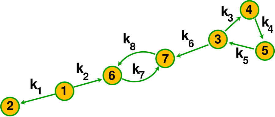
In the following, the right kernel of a matrix $A$ denotes the set of vectors $x$ so that $Ax=0$, while the left kernel is the set of (row) vectors $y$ such that $yA=0$.

Choose an arbitrary vertex $b$ as basepoint and let $r\neq b$ be any other vertex. By definition 3.7, there is an undirected path $\gamma$ from $b$ to $r$. Consider the directed edges $e_{i}$ of $\gamma$. When $\gamma$ traverses $e_{i}$ in the positive direction, multiply $e_{i}$ by $w_{i}=+1$, and in the other case by $w_{i}=-1$. The image under $\partial$ of $\sum w_{i}e_{i}$ is $r-b$. This shows that $\mathrm{Rank}\,\partial\geq v-1$. The second statement follows from the first, because the remark after Lemma 2.2 says that the sum of the two dimensions must be $v$.  

The three basic ingredients of a CRN are:

We then associate a linear vector space to each of these ingredients as follows. The column vectors $(x_{1},\cdots,x_{c})^{T}$ form the space $\mathbb{R}^{c}$. In the same way, vectors in the space $\mathbb{R}^{v}$ and $\mathbb{R}^{e}$ have components $v_{i}$ and $e_{i}$, respectively. The begin and end matrices $B$ and $E$ defined in Section 3 correspond to linear transformations $B$ and $E$ from $\mathbb{R}^{e}$ to $\mathbb{R}^{v}$, whereas their transpose acts in the opposite direction.

The spaces $\mathbb{R}^{v}$ and $\mathbb{R}^{e}$ are used to compute rates of change of concentrations, not the concentrations themselves. As an example, look at the simple system consisting of the reaction $2H_{2}+O_{2}\rightarrow 2H_{2}O$. The $x_{i}$ are the concentrations of, respectively, $H_{2}$, $O_{2}$, and $H_{2}O$. There are 2 vertices, $v_{1}$ denotes the concentration of the combination $2H_{2}+O_{2}$ and $v_{2}$ that of $2H_{2}O$ and one edge (or reaction) $v_{1}{\mathrel{\mathop{\kern 0.0pt\rightarrow}\limits^{e_{1}}}}\,v_{2}$. While the concentration of $2H_{2}+O_{2}$ is an ambiguous concept, the rate of change of that same quantity due to the reaction, is not.

Next, we describe the relationship between the reacting mixtures and the molecules. (Note that we are dropping the quotation marks.) The count of $i$-molecules in the $j$th vertex – or reacting mixture – equals $S_{ij}$. Put more simply, the $j$th column of $S$ gives the composition of molecules in the $jth$ vertex. Labeling both from left to right, the matrix $S$ for the reaction given above, is:

This defines a linear transformation $S:\mathbb{R}^{v}\rightarrow\mathbb{R}^{c}$ whose matrix has entries that are non-negative integers. In a system with many simultaneous reactions, the rate of change in $x_{i}$ (indicated by $\dot{x}_{i}$) equals the sum of the rates of change of those mixtures in which that molecule occurs. Thus

Note that if the $i$th row of $S$ is zero, then $x_{i}$ is constant and we have a redundant equation. So without loss of generality, we assume that $S$ has no zero rows.

The physical intuition behind a reaction $v_{i}{\mathrel{\mathop{\kern 0.0pt\rightarrow}\limits^{e_{\ell}}}}\,v_{j}$ in a solution of chemicals is that the reaction rate is proportional to the probability that all the necessary molecules in $v_{i}$, the tail of the arrow $e_{\ell}$, “meet” in some small volume (this is called the mass action principle). The probability that molecule $r$ is present in some small volume is proportional to $x_{r}$, its concentration in the chemical mix. Assuming these probabilities are independent of one another, we see that the probability that all the right molecules of $v_{i}$ are present in the small volume equals the product of all the concentrations of the molecules in $v_{i}$. This product is called $\psi_{i}(X)$, and these form a vector $\psi(x)$ in $\mathbb{R}^{v}$. With the above definition of $S$, we see that this product is proportional to $\prod_{j}x_{j}^{S_{ji}}$. We thus define a vector in vertex space $\mathbb{R}^{v}$ (using the convention that $0^{0}:=1$):

Next, we transform $\psi\in\mathbb{R}^{v}$ to the vector in the edge space $\mathbb{R}^{e}$ whose $\ell$th component is the reaction rate of the $\ell$th reaction $v_{i}{\mathrel{\mathop{\kern 0.0pt\rightarrow}\limits^{e_{\ell}}}}\,v_{j}$. From the previous paragraph, we conclude that the rate of the $\ell$th reaction is proportional to $\psi_{i}(x)$, where the $i$th vertex is the tail (the begin point) of the $\ell$th directed edge. Thus using the begin matrix $B$ of Section 3, we see that the reaction rates are proportional to

In the chemical literature, this proportionality is (nearly) always expressed by a constant called $k$. It is important to note that this constant is associated with the $\ell$th reaction – or edge – and not with the reacting mixture – or begin vertex – of that reaction. Thus we weight the edges using an $e\times e$ diagonal matrix $W$ whose $\ell$th diagonal element equals a (strictly) positive constant $k_{\ell}$. The reaction rates are therefore given by

The reaction $v_{i}{\mathrel{\mathop{\kern 0.0pt\rightarrow}\limits^{e_{\ell}}}}\,v_{j}$ adds to the concentration of mixture $v_{j}$ and subtracts from the concentration of mixture $v_{i}$, both at the rate $k_{\ell}\psi_{\ell}$. Again, with the definitions of $E$ and $B$ of Section 3, we compute the rates of change of the concentration reacting mixtures $v\in\mathbb{R}^{v}$ as:

Finally, in chemical situations we can’t necessarily measure or observe directly the concentrations of reacting mixtures. Rather, we observe the concentrations of the various molecules $x_{i}$. Applying (4.1) gives us the final form of the dynamical system in $\mathbb{R}^{c}$ associated to chemical reaction networks

Solutions of this system can also be derived from the solutions of the following system:

where we used (4.1). Interestingly, the reverse is not necessarily true. A solution of (4.3) does not always determine a unique solution of (4.4). In fact, one of the problems that comes up in this type of system, is whether non-trivial reactions can take place even though $\dot{x}=0$. From the above equations one can see that could happen if during these reactions $\dot{v}\in\mathrm{Ker}\,S$. This is of course impossible if $\mathrm{Ker}\,S\cap\mathrm{Im}\,L_{\mathrm{out}}^{T}=0$, as we will see in Section 5.

To summarize the whole framework schematically, here is a diagram of the transformations involved in (4.3).

The important step here is that we split these transformations into a non-linear part $\psi(x)$ and a linear part $-SL_{\mathrm{out}}^{T}$. In the literature, however, since the revolutionary work done in the 1970’s [16, 17, 10], the traditional split in treatment has been between $S\partial$ on the one hand and $WB^{T}\psi$ on the other. This was done, because the weights in $W$ are the reaction rates and these are notoriously difficult to measure. In addition, of course, one did not have access to Theorems 3.5 and 3.6. And so some of the linear transformations — to wit: $WB^{T}$ in (4.5) — were lumped with the non-linear part $\psi$. What we exhibit in this work is the price paid for that choice.

Our next result is a reality check. Since concentrations cannot be negative, we want to make sure that the set $\mathbb{R}^{c}_{+}=\{x\in\mathbb{R}^{c}\,|\,\forall i\;:\;x_{i}\geq 0\}$, also called the positive orthant, is forward invariant.

So suppose $x_{j}=0$. Since $S$ has no zero rows, there must be a $i$ such that $S_{ji}$ is a positive integer. From (4.2) we see that for all $i$ such that then $S_{ji}>0$, we have $\psi_{i}=0$. The off-diagonal elements of $-L_{\mathrm{out}}^{T}$ are non-negative, and so for these same $i$

Using again that $S_{ji}$ is non-negative, we have

This proves the proposition.  

The preceding development shows that an out-degree Laplacian arises naturally in the analysis of CRNs. We will see that the algebraic results in Section 3 are of great use in this analysis. However to make use of them, we will need to adapt them to the out-degree Laplacian. Fortunately, this is extremely simple thanks to the dual relationship between the two, namely $L_{\mathrm{out}}(G)=L_{\mathrm{in}}(G^{\Lsh})$ noted in definition 3.1. Theorems 3.4, 3.5, and 3.6 hold for $L_{\mathrm{out}}$ if we replace each instance of reach and cabal with the dual notions of co-reach and co-cabal.

It turns out that in the development of our theory, we do not use the fact that $S$ is an integer matrix nor the fact that the Laplacian is out-degree. Hence in the next few sections, we consider the following slightly more general problem.

Equation (4.3) implies that $\dot{x}\in\mathrm{Im}\,SL_{\mathrm{}}^{T}$. Thus the orthogonal projection of $x$ to $\left(\mathrm{Im}\,SL_{\mathrm{}}^{T}\right)^{\perp}=\mathrm{Ker}\,L_{\mathrm{}}S^{T}$ is in fact a constant of the motion. This motivates the following definition.

We present two definition for the deficiency of a network. The fact that they are equal follows from Proposition 2.4.

The next result shows that a 0 deficiency network has a strictly positive equilibrium if and only if it is CSC. In the two sections that follow we will refine this to show that if a 0 deficiency network is CSC, then every invariant set $X_{z}$ (Definition 4.2) has a unique equilibrium (Theorem 6.4) and furthermore, that equilibrium is asymptotically stable (Theorem 7.3).

Now we prove $\Longleftarrow$. Suppose that every reach is a strong component, then using $\delta_{L}=0$ we must show that (5.1) has a positive solution $\psi^{*}$ with $x^{*}>0$. By positivity, we can take the componentwise logarithm of both sides. We note that $\mathrm{Ln}\,\psi(x^{*})=S^{T}\mathrm{Ln}\,x^{*}$. The logarithm of the right hand side of (5.1) can be written as

where $\mathbf{1_{R_{m}}}$ is the characteristic vector of the $m$th reach or (in this case) component. Note that $\sum_{m=1}^{k}\bar{\gamma}_{m}$ has all components positive by assumption. Thus from (5.1) we see that we need to solve $x^{*}$ in

This can be re-arranged as

We observe that the first term of the right hand side ranges over $\mathrm{Im}\,S^{T}$ and the second over $\mathrm{Ker}\,L_{\mathrm{}}$. This has a solution if

However, this is guaranteed by applying Proposition 2.3 to the zero deficiency condition.  

This is the analogue of the classical zero deficiency theorem. It can, however, be strengthened significantly with very little effort. Here we first show that once can weaken the existence of an positive equilibrium to the existence of an orbit $x(t)$ such that $\mathrm{Ln}\,x(t)$ is bounded. Secondly, even if the zero deficiency system is not CSC, we can still write down equations that determine all the equilibria of the dynamics in each $X_{z}$ of Definition 4.2. In Sections 6 and 7, we will furthermore show existence and uniqueness as well as asymptotic stability of these equilibria.

Two comments are in order here. The first is that Theorems 5.3 and 5.4 imply that for a deficiency zero system $S$ with associated graph $G$ the following holds:

In particular, for a (Laplacian) deficiency zero system, we have that that CSC implies that none of the concentrations $x_{i}$ tend to zero. The persistence conjecture [11] says that this is true independently of the deficiency.

We will show that a CRN whose associated graph is CSC with zero Laplacian deficiency has exactly one positive equilibrium in each invariant set $X_{z}$ (see Definition 4.2). Informally speaking, then, the set of equilibria forms a graph (as in: is a function of) over $\mathrm{Ker}\,L_{\mathrm{}}S^{T}$. The precise formulation is given below in Theorem 6.4. (See the last paragraph of the introduction for the notation.)

To accomplish this, fix $x^{*}$ and $z$ as above and define $g:\mathbb{R}^{c}\rightarrow\mathbb{R}$ by setting

This function is a sum of $c$ one-dimensional functions described in Lemma 2.7. This Lemma implies that there is a box $B=[\mu_{1,-},\mu_{1,+}]\times\cdots\times[\mu_{c,-},\mu_{c,+}]\subseteq\mathbb{R}^{c}$ so that

See Figure 6.1. Therefore the set $C$ defined by

is non-empty (as it contains 0), closed (by continuity of $g$), and bounded.

Now we restrict $g$ to $\mathrm{Ker}\,L_{\mathrm{}}S^{T}$. Since $0\in\mathrm{Ker}\,L_{\mathrm{}}S^{T}$, the continuous function $g$ assumes its minimum in $\mathrm{Ker}\,L_{\mathrm{}}S^{T}$ at a point $\mu^{*}$. Since $g$ is also differentiable, at $\mu=\mu^{*}$, we must have

which establishes equation (6.1), thereby proving the proposition.

References

- [1] D. F. Anderson. A proof of the global attractor conjecture in the single linkage class case. SIAM Journal on Applied Mathematics, 71(4):1487–1508, 2011.
- [2] R. Aris. Prolegomena to the rational analysis of systems of chemical reactions. Archive for Rational Mechanics and Analysis, 19(2):81–99, 1965.
- [3] B. Bollobás. Modern Graph Theory. Springer, 1998.
- [4] W. C. Bray. A periodic reaction in homogeneous solution and its relation to catalysis. Journal of the American Chemical Society, 43(6):1262–1267, 1921.
- [5] J. D. Brunner and G. Craciun. Robust persistence and permanence of polynomial and power law dynamical systems. SIAM Journal on Applied Mathematics, 78(2):801–825, 2018.
- [6] J. S. Caughman and J. J. P. Veerman. Kernels of directed graph Laplacians. The Electronic Journal of Combinatorics, 13(1), 2006.
- [7] P. Chebotarev and R. Agaev. Forest matrices around the Laplacian matrix. Linear Algebra and its Applications, 356(1-3):254–273, 2002.
- [8] G. Craciun, A. Dickenstein, A. Shiu, and B. Sturmfels. Toric dynamical systems. Journal of Symbolic Computation, 44(11):1551–1565, 2009.
- [9] A. Dickenstein. Algebraic geometry tools in systems biology. Notices of the American Mathematical Society, 67:1706–1715, 2021.
- [10] M. Feinberg. Complex balancing in general kinetic systems. Archive for Rational Mechanics and Analysis, 49(3):187–194, 1972.
- [11] M. Feinberg. Chemical reaction network structure and the stability of complex isothermal reactors—i. the deficiency zero and deficiency one theorems. Chemical Engineering Science, 42(10):2229–2268, 1987.
- [12] M. Feinberg. The existence and uniqueness of steady states for a class of chemical reaction networks. Archive for Rational Mechanics and Analysis, (132):311–370, 1995.
- [13] M. Feinberg. Foundations of chemical reaction network theory. Springer, 2019.
- [14] M. Feinberg and F. J. M. Horn. Dynamics of open chemical systems and the algebraic structure of the underlying reaction network. Chemical Engineering Science, 29(3):775–787, 1974.
- [15] J. Gunawardena. Chemical reaction network theory for in-silico biologists. Available online: http://vcp.med.harvard.edu/papers/crnt.pdf, 2003.
- [16] F. J. M. Horn. Necessary and sufficient conditions for complex balancing in chemical kinetics. Archive for Rational Mechanics and Analysis, 49(3):172–186, 1972.
- [17] F. J. M. Horn and R. Jackson. General mass action kinetics. Archive for Rational Mechanics and Analysis, 47(2):81–116, 1972.
- [18] B. Joshi and A. Shiu. Which small reaction networks are multistationary? SIAM Journal on Applied Dynamical Systems, 16(2):802–833, 2017.
- [19] M. Kaufman and C. Soulé. On the multistationarity of chemical reaction networks. Journal of Theoretical Biology, 465:126–133, 2019.
- [20] Y. Kim, J. W. Kim, Z. Kim, and W. Y. Kim. Efficient prediction of reaction paths through molecular graph and reaction network analysis. Chemical Science, 9(4):825–835, 2018.
- [21] I. Mirzaev and J. Gunawardena. Laplacian dynamics on general graphs. Bulletin of Mathematical Biology, 75(11):2118–2149, sep 2013.
- [22] F. Pucci and M. Rooman. Deciphering noise amplification and reduction in open chemical reaction networks. Journal of The Royal Society Interface, 15(149):20180805, dec 2018.
- [23] S. Rao, A. J. Van Der Schaft, and B. Jayawardhana. A graph-theoretical approach for the analysis and model reduction of complex-balanced chemical reaction networks. Journal of Mathematical Chemistry, 51(9):2401–2422, 2013.
- [24] A. J. Van Der Schaft, S. Rao, and B. Jayawardhana. A network dynamics approach to chemical reaction networks. International Journal of Control, 89(4):731–745, 2015.
- [25] A. Shiu and B. Sturmfels. Siphons in chemical reaction networks. Bulletin of Mathematical Biology, 72(6):1448–1463, jan 2010.
- [26] E. D. Sontag. Structure and stability of certain chemical networks and applications to the kinetic proofreading model of T-cell receptor signal transduction. Automatic Control, IEEE Transactions on, 46:1028 – 1047, 08 2001.
- [27] E. D. Sontag. Correction to “structure and stability of certain chemical networks and applications to the kinetic proofreading model of T-cell receptor signal transduction”. IEEE Trans Aut Control, 47(4):1028–1047, 2002.
- [28] S. Sternberg. Dynamical Systems. Dover, 2010, revised 2013.
- [29]
J. J. P. Veerman.
Digraphs IV.
Available online:
http://web.pdx.edu/~veerman/2019-Digraphs-4.pdf, 2019. - [30] J. J. P. Veerman and E. Kummel. Diffusion and consensus on weakly connected directed graphs. Linear Algebra and its Applications, 578:184–206, 2019.
- [31] J. J. P. Veerman and R. Lyons. A primer on Laplacian dynamics in directed graphs. Nonlinear Phenomena in Complex Systems, 23(2), 2020.
- [32] L. Wang and E. D. Sontag. On the number of steady states in a multiple futile cycle. J. Math. Biol., 1(57):29–52, 2008.
- [33] R. Wegscheider. Ueber simultane Gleichgewichte und die Beziehungen zwischen Thermodynamik und Reactionskinetik homogener Systeme. Monatshefte fuer Chemie, 8(32):849–906, 1901.
- [34] A. T. Winfree. The prehistory of the Belousov-Zhabotinsky oscillator. J. Chem. Educ., (61):661–663, 1984.
- [35] A. M. Zhabotinsky. A history of chemical oscillations and waves. Chaos: An Interdisciplinary Journal of Nonlinear Science, 1(4):379–386, dec 1991.