Maximum efficiency of absorption refrigerators at arbitrary cooling power

Below, we will optimise the efficiency of the CAR with respect to durations $t_{\rm e}$ and $t_{\rm r}$ of the engine and refrigeration cycles and thus we assume that they are different. Duration of one cycle of the CAR, $t_{\rm s}$, is defined as a period after which both the internal devices attain their initial states. It is thus given by the least common multiple of $t_{\rm e}$ and $t_{\rm r}$. We assume that such a common multiple exists and denote as

($N_{\rm r}=t_{\rm s}/t_{\rm r}$) the number of engine (refrigeration) cycles performed per one full CAR cycle.

Now we are ready to define the thermodynamic quantities of interest, sketched in Fig. 1. Per CAR cycle, the engine produces work $W=N_{\rm e}W_{\rm e}$, which is used by the refrigerator to pump heat $N_{\rm r}Q_{\rm c}$ from the cold bath. Output power of the engine $W/t_{\rm s}$ and the input power of the refrigerator thus reads

where $W_{\rm r}=W/N_{\rm r}$ denotes the work used by the refrigerator per refrigeration cycle.

According to the first law, we have $W_{\rm e}=Q_{\rm h}-Q_{\rm me}$ and $Q_{\rm c}=Q_{\rm mr}-W_{\rm r}$. Here, $Q_{\rm h}$ and $Q_{\rm me}$ are the heats taken from the hot bath and delivered to the intermediate bath by the engine per period $t_{\rm e}$, respectively. Similarly, $Q_{\rm mr}$ is heat pumped into the intermediate bath by the refrigerator per period $t_{\rm r}$. The amount of heat extracted by the internal refrigerator from the cold bath per CAR cycle is given by $N_{\rm r}Q_{\rm c}$. The cooling power of the simultaneous CAR, $R_{\rm s}$, and the internal refrigerator, $R$, are thus the same and read

The energy input of the CAR is $N_{\rm e}Q_{\rm h}$ and thus its efficiency, referred to as the coefficient of performance (COP), is given by

Here, $\eta=W_{\rm e}/Q_{\rm h}$ and $\varepsilon=Q_{\rm c}/W_{\rm r}=R/P$ denote the efficiency of the internal heat engine and refrigerator, respectively.

Before we turn our attention to the MEGP for CARs, we determine the interval of allowed values of the cooling power (4). Its minimum value 0 is achieved for infinitely slow cycles. The maximum cooling power, $R^{*}_{\rm s}$, turns out to be limited by maximum powers of both constituting devices.

The power source of the refrigerator inside the CAR is the internal heat engine and thus the maximum cooling power of the CAR can not be larger than the maximum cooling power of the internal refrigerator without restrictions to input power, $R^{*}$, i.e. $R^{*}_{\rm s}\leq R^{*}$. Furthermore, the cooling power is related to output power of the engine by

We denote as $\bar{R}$ the maximum value of cooling power solving the equation

where $P^{*}$ is the maximum power of the engine. If $\bar{R}<R^{*}$, the engine is not powerful enough to utilize the whole potential of the refrigerator and $R^{*}_{\rm s}=\bar{R}$. Similarly, $\bar{R}>R^{*}$ means that the refrigerator is not powerful enough to use the whole power provided by the engine and $R^{*}_{\rm s}=R^{*}$. Altogether, we found that the maximum power of the CAR is given by

In the next section, we finally discuss the MEGP for the simultaneous CARs.

Inserting Eq. (6) for engine output power as function of power of the refrigerator in Eq. (5), we obtain the COP of the CAR as function of $R$:

To get the MEGP for CAR, we need to optimize the right-hand-side of this equation with respect to the durations of $t_{\rm r}$ and $t_{\rm e}$ for fixed $R$. Using Eqs. (6), (34), and (48), Eq. (9) can be rewritten in the form

where $\eta_{\rm C}$ and $\varepsilon_{\rm C}$ are Carnot efficiency of reversible Carnot heat engine and refrigerator, respectively, i.e. $\eta_{\rm C}=1-T_{\rm m}/T_{\rm h}$, and $\varepsilon_{\rm C}=T_{\rm c}/(T_{\rm m}-T_{\rm c})$, and

is the sum of average entropy production rates in the internal heat engine and internal refrigerator and thus the total average entropy production rate during the CAR cycle. Expressions for the total entropy changes per engine and refrigeration cycle, $\Delta S_{\rm tot,r}$ and $\Delta S_{\rm tot,e}$ are given in Eqs. (35) and (49) in the appendix. Maximization of COP (9) at fixed $R$ is thus equivalent to minimization of the average entropy production rate $\sigma=\sigma(R)$ under the same conditions.

The internal heat engine depends on the setup and performance of the refrigerator through the refrigeration power $R/\varepsilon(R)$ only. Thus, in order to yield the maximum value of the product in Eq. (9), $\eta(R/\varepsilon(R))$ must attain its maximal value, $\eta^{\rm opt}(R/\varepsilon(R))$, corresponding to the given refrigeration power (MEGP). Furthermore, all known expressions for MEGP are decreasing functions of power Holubec and Ryabov 2016; Holubec and Ye 2020; Ryabov and Holubec 2016; Long et al. 2018; Long and Liu 2016. Importantly, all these models neglect losses, which cannot be avoided by quasi-static operation, such as heat leakages, and thus they can saturate the Carnot bound on efficiency in the limit of vanishing power. Assuming that this idealization holds also in our present case, $\eta^{\rm opt}(R/\varepsilon(R))$ will be maximal if $\varepsilon(R)$ will be given by the maximum refrigerating efficiency at the given power, $\varepsilon^{\rm opt}(R)$. Altogether, the MEGP for the considered idealized CARs reads

The MEGP for the simultaneous CAR thus in general follows from the expressions for MEGPs for the internal engine and refrigerator. Let us now consider the simultaneous CAR composed of a LD heat engine and LD refrigerator Holubec and Ryabov 2016; Holubec and Ye 2020. For this specific model, we verified validity of Eq. (12) by direct numerical maximisation of Eq. (9). In the next section, we utilise known analytical expressions for $\eta^{\rm opt}$ and $\varepsilon^{\rm opt}$ for this model to discuss in detail properties of the MEGP (9) for this LD CAR based on analytical grounds.

The MEGP for the LD CAR follows from Eq. (12) after inserting the expressions for MEGP of the internal LD heat engine, $\eta^{\rm opt}$, and refrigerator, $\varepsilon^{\rm opt}$. For the engine, we derive $\eta^{\rm opt}$ in the Appx. B. Similarly as the derivation given in Ref. Holubec and Ryabov 2016, our present approach involves an approximation in calculation of the optimal redistribution of the total cycle duration between the two isothermal branches. Nevertheless, our analytical result for $\eta^{\rm opt}$ is, within the numerical precision, indistinguishable from the corresponding result obtained by exact numerical optimisation of the efficiency. For the refrigerator, we review in Appx. C the derivation of analytical expression for $\varepsilon^{\rm opt}$ from Ref. Holubec and Ye 2020.

All results for MEGP available in the literature Long et al. 2018; Holubec and Ryabov 2015; Long and Liu 2016; Ryabov and Holubec 2016; Holubec and Ryabov 2016; Holubec and Ye 2020; Holubec and Ryabov 2017 are given as functions of the dimensionless variable

measuring how much power is lost by operating the device at power $X$ smaller than the maximum power $X^{*}$. In our case, we have three such variables: the loss in power of the internal engine, $\delta P$, the loss in cooling power of the internal refrigerator, $\delta R$, and the loss in cooling power of the CAR, $\delta R_{\rm s}$. In general, these variables can assume values from the interval $[-1,0]$. The minimum is attained if the actual power is negligible compared to the maximum power and the maximum corresponds to devices operating at maximum power. However, in our specific setting where the input power of the refrigerator can be limited by the output power of the engine, the upper bound for $\delta R$ reads $R_{\rm s}^{*}/R^{*}-1\leq 0$.

In order to insert the known results for MEGP of the refrigerator and heat engine into Eq. (12), we need to express them in terms of refrigeration power $R$ and engine output power $P=R/\varepsilon^{\rm opt}(R)$, respectively. From now on, we use the shorthand notation $\varepsilon^{\rm opt}(\delta R)\equiv\varepsilon^{\rm opt}[R(\delta R)]$, where $R(\delta R)=(1+\delta R)R^{*}$, and similarly for $\eta^{\rm opt}(\delta P)$. Furthermore, in order to be able to discuss the MEGP of the CAR, $\psi^{\rm opt}=\varepsilon^{\rm opt}(\delta R)\eta^{\rm opt}(\delta P)$, as a function of the loss in cooling power of the CAR, we use Eqs. (6) and (17) to express $\delta P$ and $\delta R$ in terms of $\delta R_{\rm s}$. The result is

where we introduced the reduced maximum powers of the engine, $\tilde{P}^{*}=P^{*}/R^{*}$, and the CAR, $\tilde{R}_{\rm s}^{*}=R_{\rm s}^{*}/R^{*}$, measured in units of maximum power of the internal refrigerator.

When expressed in terms of $\delta P$, the MEGP of the LD heat engine, $\eta^{\rm opt}$, depends only on the ratio of the irreversibility parameters, $\Sigma_{\rm e}=\Sigma_{\rm h}/\Sigma_{\rm me}$, Carnot efficiency, $\eta_{\rm C}$, and $\delta P$. For details, see Appx. B. Similarly, we show in Appx. C that $\varepsilon^{\rm opt}$ is only a function of $\Sigma_{\rm r}=\Sigma_{\rm mr}/\Sigma_{\rm c}$, $\varepsilon_{\rm C}=T_{\rm c}/(T_{\rm m}-T_{\rm c})$, and $\delta R$. Since the MEGP, $\varepsilon^{\rm opt}(R)$, is a monotonously decreasing function of $R$, the ratio $R/\varepsilon^{\rm opt}(R)$ attains its maximum value for $R^{*}$. Therefore, Eqs. (7) and (8) imply that the reduced maximum power of the CAR $\tilde{R}_{\rm s}^{*}$ is given by

if the resulting $\tilde{R}^{*}_{\rm s}$ is smaller than one, and by $\tilde{R}^{*}_{\rm s}=1$ otherwise. Hence $\tilde{R}^{*}_{\rm s}$ is determined by $\Sigma_{\rm r}$, $\varepsilon_{\rm C}$, and $\tilde{P}^{*}$. Collecting all these results and inserting them into Eq. (12), we can finally write the MEGP of the LD simultaneous CAR in terms of the relative loss in its maximum cooling power, $\delta R_{\rm s}$. The resulting expression depends on the six parameters introduced above, namely

In the following sections, we use this expression to provide more explicit results on MEGP of CARs.

We start by deriving maximum and minimum values of the optimal COP $\psi^{\rm opt}$ with respect to working medium of the CAR (or of its constituents). In the LD approximation, the detailed physics of the working medium is described by the irreversibility parameters $\Sigma_{\rm i}$, $i=$ h, me, c, mr defined by Eqs. (13)–(16) Schmiedl and Seifert 2007; Sekimoto and Sasa 1997; Holubec and Ryabov 2015; Abiuso and Perarnau-Llobet 2020; Abiuso et al. 2020.

The optimal COP (21) depends on irreversibility parameters through the ratios $\Sigma_{\rm e}=\Sigma_{\rm h}/\Sigma_{\rm me}$ and $\Sigma_{\rm r}=\Sigma_{\rm mr}/\Sigma_{\rm c}$ and the reduced maximum power of the internal engine $\tilde{P}^{*}$. With respect to the former two, the optimal COP attains its minimum for $\Sigma_{\rm e}\to 0$ (hot isotherm of the internal engine cycle is reversible compared to the other one) and $\Sigma_{\rm r}\to\infty$ (cold isotherm of the refrigeration cycle is reversible compared to the other one). Its maximum $\psi^{\rm opt}$ is attained in the opposite limit $\Sigma_{\rm e}\to\infty$ and $\Sigma_{\rm r}\to 0$. Taking these limits into Eq. (21), we find the lower and upper bounds for the optimal COP:

This inequality has to be further optimized with respect to the parameter $\tilde{P}^{*}$, which enters the upper bound through Eqs. (18) and (19) for $\delta P$ and $\delta R$, respectively. Note that due to the limits $\Sigma_{\rm e}\to\infty$ and $\Sigma_{\rm r}\to 0$ taken to derive the upper bound, we have to use $\varepsilon^{\rm opt}=\varepsilon_{+}^{\rm opt}$ defined in Eq. (60) in the formula for $\delta P$. One finds that the upper bound is a monotonously decreasing function of $\tilde{P}^{*}$ and thus its maximum is obtained for $\tilde{P}^{*}=0$. The resulting ultimate bounds on the optimal COP of the CAR at given cooling power read

The upper bound evaluated for $\delta R_{\rm s}=0$, $\psi^{\rm opt}_{+}(0)=\varepsilon_{\rm C}\eta_{\rm C}/(2-\eta_{\rm C})$, denotes the upper bound for COP of the CAR at maximum cooling power.

The increase in COP gained after a slight decrease of the cooling power from its maximum value can be measured by the expression

Its derivative with respect to $\delta R_{\rm s}$ diverges, implying that a slight decrease of the cooling power leads to a significant gain in the upper bound on COP. Qualitatively the same behavior has generally been observed for MEGPs of various heat engines Long and Liu 2016; Ryabov and Holubec 2016; Holubec and Ryabov 2016; Dechant et al. 2017; Whitney 2014; Whitney 2015. With respect to LD refrigerators, the MEGP is proportional to $\sqrt{-\delta R}$ for a limited range of parameters only and behaves as $\propto-\delta R$ otherwise Holubec and Ye 2020. In the next section, we investigate whether the increase of MEGP for the CAR behaves for small values of $\delta R_{\rm s}$ always like the MEGPs in heat engines Holubec and Ryabov 2016 or if it sometimes also exhibits the linear behavior observed in refrigerators Holubec and Ye 2020.

Examples of parameter regimes where the MEGP for LD refrigerators exhibits the two qualitatively different behaviors are $\Sigma_{\rm r}\to 0$ (square root) and $\Sigma_{\rm r}\to\infty$ (linear) Holubec and Ye 2020. We thus investigate behavior of the MEGP for the CAR (21) in these two regimes using the cumbersome analytical expressions derived in Appendixes B and C.

Outside the limiting parameter regimes discussed above, the full analytical expression (21) for the MEGP is too cumbersome to get an immediate insight into the behavior of $\psi^{\rm opt}$. Therefore, in this section, we investigate its dependence on the model parameters graphically.

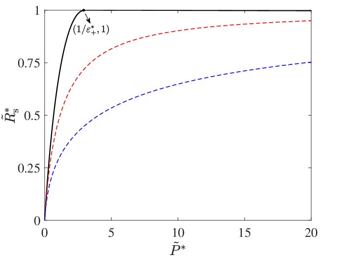
In Fig. 3, we show the reduced maximum power of the CAR, $\tilde{R}_{\rm s}^{*}$, as a function of the reduced power of the internal heat engine, $\tilde{P}^{*}$. The larger the available input power of the refrigerator (provided by the engine) the larger the corresponding maximum cooling power until the latter reaches its maximum, $\tilde{R}_{\rm s}^{*}=1$, where the whole cooling potential of the internal refrigerator is utilized. The minimum value of the reduced power, $\tilde{P}^{*}=1/\varepsilon^{\rm opt}(0)$, allowing for $\tilde{R}_{\rm s}^{*}=1$ follows from Eq. (20). Here, $\varepsilon^{\rm opt}(0)=\varepsilon^{*}_{\pm}$ denotes the MEGP for the refrigerator defined in Eqs. (52) and (53). Hence, $\tilde{R}_{\rm s}^{*}=1$ for finite value ($\tilde{P}^{*}=1/\varepsilon_{+}^{*}$) of the reduced power only if $\Sigma_{\rm r}=0$, i.e., when the dissipation during the hot isotherm of the refrigeration cycle becomes negligible compared to that during the cold one. For $\Sigma_{\rm r}>0$, the whole cooling potential of the internal refrigerator can be utilized only for infinite values of the reduced power, $\tilde{P}^{*}=1/\varepsilon_{-}^{*}\to\infty$. This is caused by the discontinuity in the ability of the refrigerator working at maximum power conditions to utilize the energy provided by the engine, $\varepsilon^{\rm opt}(0)$, which is positive for $\Sigma_{\rm r}=0$ and vanishes for $\Sigma_{\rm r}>0$ Holubec and Ye 2020. Figure 3 also shows that, for fixed $\tilde{P}^{*}$ and $\varepsilon_{\rm C}$, $\tilde{R}_{\rm s}^{*}$ decreases as the amount of energy dissipated during the hot isotherm of the refrigeration cycle increases (larger $\Sigma_{\rm r}$).

In Fig. 4, we plot the MEGP for CARs (21) as a function of $\delta R_{\rm s}$ for different values of $\tilde{P}^{*}$, $\Sigma_{\rm e}$, and $\Sigma_{\rm r}$. The upper bounds (22) for MEGP for fixed reduced power $\tilde{P}^{*}$ are depicted for $\tilde{P}^{*}=1$ (upper pink line) and $\tilde{P}^{*}\geq 1/\varepsilon_{+}^{*}$ (lower pink line). They indeed bound the MEGP obtained for arbitrary values of ratios of irreversibility parameters $\Sigma_{\rm e}$ and $\Sigma_{\rm r}$, and values of $\tilde{P}^{*}$ smaller than those chosen to plot the individual curves. The ultimate upper bound on MEGP (23) is depicted by the uppermost black solid line. According to the figure, the MEGP $\psi^{\rm opt}$ exhibits a fast nonlinear increase with decreasing power near $\delta R_{\rm s}\to 0$ unless $\tilde{P}^{*}\to\infty$. Only then this increase is linear, in agreement with our discussion below Eq. (28). In order to check our analytical results, we also calculated the MEGP for simultaneous LD CARs by a direct brute-force numerical optimization of COP (5). The figure shows that the obtained numerical results (symbols) perfectly overlap with our analytical predictions (lines).

In Fig. 5, we show the characteristics of the heat engine and refrigerator corresponding to the MEGP of the CAR with $\Sigma_{\rm r}=\Sigma_{\rm e}=1$, depicted in Fig. 4. For $\tilde{P}^{*}\to 0$, Eqs. (18)-(20) imply that $\delta R=-1$, $\varepsilon^{\rm opt}=\varepsilon_{\rm C}$, and $\delta P=\delta R_{\rm s}$. Similarly, for $\tilde{P}^{*}\to\infty$ it follows that $\delta R=\delta R_{\rm s}$, $\delta P=-1$, and $\eta^{\rm opt}=\eta_{\rm C}$. When the refrigerator works at the Carnot COP $\varepsilon_{\rm C}$, the dimensionless refrigeration cycle duration $\tau_{\rm r}^{\rm opt}$ diverges and we have $N_{\rm e}/N_{\rm r}\to\infty$, i.e. within one full CAR cycle, there is infinitely more engine cycles than refrigeration cycles. An opposite situation occurs when the engine works at Carnot efficiency.

References

- Callen (2006) H. B. Callen, Thermodynamics and an Introduction to Thermostatistics, Student Edition (Wiley India Pvt. Ltd, 2006).
- Holubec and Ryabov (2017) V. Holubec and A. Ryabov, Diverging, but negligible power at carnot efficiency: Theory and experiment, Phys. Rev. E 96, 062107 (2017).
- Müller (2007) I. Müller, A History of Thermodynamics: The Doctrine of Energy and Entropy (Springer, 2007).
- Yvon (1955) J. Yvon, Saclay Reactor: Acquired knowledge by two years experience in heat transfer using compressed gas, Tech. Rep. (CEA Saclay, 1955).
- Chambadal (1957) P. Chambadal, Les centrales nucléaires, Vol. 321 (Colin, 1957).
- Novikov (1958) I. I. Novikov, The efficiency of atomic power stations (a review), J. Nucl. Energy II 7, 125 (1958).
- Esposito et al. (2010a) M. Esposito, R. Kawai, K. Lindenberg, and C. Van den Broeck, Efficiency at maximum power of low-dissipation carnot engines, Phys. Rev. Lett. 105, 150603 (2010a).
- Gonzalez-Ayala et al. (2020) J. Gonzalez-Ayala, J. Guo, A. Medina, J. M. M. Roco, and A. C. Hernández, Energetic self-optimization induced by stability in low-dissipation heat engines, Phys. Rev. Lett. 124, 050603 (2020).
- Wang et al. (2012) Y. Wang, M. Li, Z. C. Tu, A. C. Hernández, and J. M. M. Roco, Coefficient of performance at maximum figure of merit and its bounds for low-dissipation carnot-like refrigerators, Phys. Rev. E 86, 011127 (2012).
- Van den Broeck (2005) C. Van den Broeck, Thermodynamic efficiency at maximum power, Phys. Rev. Lett. 95, 190602 (2005).
- Benenti et al. (2011) G. Benenti, K. Saito, and G. Casati, Thermodynamic bounds on efficiency for systems with broken time-reversal symmetry, Phys. Rev. Lett. 106, 230602 (2011).
- Izumida and Okuda (2014) Y. Izumida and K. Okuda, Work output and efficiency at maximum power of linear irreversible heat engines operating with a finite-sized heat source, Phys. Rev. Lett. 112, 180603 (2014).
- Izumida et al. (2015) Y. Izumida, K. Okuda, J. M. M. Roco, and A. C. Hernández, Heat devices in nonlinear irreversible thermodynamics, Phys. Rev. E 91, 052140 (2015).
- Izumida and Okuda (2012) Y. Izumida and K. Okuda, Efficiency at maximum power of minimally nonlinear irreversible heat engines, EPL 97, 10004 (2012).
- Schmiedl and Seifert (2007) T. Schmiedl and U. Seifert, Efficiency at maximum power: An analytically solvable model for stochastic heat engines, EPL 81, 20003 (2007).
- Segal (2008) D. Segal, Stochastic pumping of heat: Approaching the carnot efficiency, Phys. Rev. Lett. 101, 260601 (2008).
- Jarzynski and Mazonka (1999) C. Jarzynski and O. Mazonka, Feynman’s ratchet and pawl: An exactly solvable model, Phys. Rev. E 59, 6448 (1999).
- Esposito et al. (2009a) M. Esposito, K. Lindenberg, and C. Van den Broeck, Universality of efficiency at maximum power, Phys. Rev. Lett. 102, 130602 (2009a).
- Esposito et al. (2009b) M. Esposito, K. Lindenberg, and C. Van den Broeck, Thermoelectric efficiency at maximum power in a quantum dot, EPL 85, 60010 (2009b).
- Esposito et al. (2010b) M. Esposito, R. Kawai, K. Lindenberg, and C. Van den Broeck, Quantum-dot carnot engine at maximum power, Phys. Rev. E 81, 041106 (2010b).
- Nakpathomkun et al. (2010) N. Nakpathomkun, H. Q. Xu, and H. Linke, Thermoelectric efficiency at maximum power in low-dimensional systems, Phys. Rev. B 82, 235428 (2010).
- Whitney (2014) R. S. Whitney, Most efficient quantum thermoelectric at finite power output, Phys. Rev. Lett. 112, 130601 (2014).
- Whitney (2015) R. S. Whitney, Finding the quantum thermoelectric with maximal efficiency and minimal entropy production at given power output, Phys. Rev. B 91, 115425 (2015).
- Holubec and Ryabov (2015) V. Holubec and A. Ryabov, Efficiency at and near maximum power of low-dissipation heat engines, Phys. Rev. E 92, 052125 (2015).
- Holubec and Ryabov (2016) V. Holubec and A. Ryabov, Maximum efficiency of low-dissipation heat engines at arbitrary power, J. Stat. Mech. 2016, 073204 (2016).
- Ryabov and Holubec (2016) A. Ryabov and V. Holubec, Maximum efficiency of steady-state heat engines at arbitrary power, Phys. Rev. E 93, 050101 (2016).
- Dechant et al. (2017) A. Dechant, N. Kiesel, and E. Lutz, Underdamped stochastic heat engine at maximum efficiency, EPL 119, 50003 (2017).
- Apertet et al. (2013) Y. Apertet, H. Ouerdane, A. Michot, C. Goupil, and P. Lecoeur, On the efficiency at maximum cooling power, EPL 103, 40001 (2013).
- Yan and Chen (1990) Z. Yan and J. Chen, A class of irreversible carnot refrigeration cycles with a general heat transfer law, J. Phys. D 23, 136 (1990).
- de Tomás et al. (2012) C. de Tomás, A. C. Hernández, and J. M. M. Roco, Optimal low symmetric dissipation carnot engines and refrigerators, Phys. Rev. E 85, 010104 (2012).
- Hernández et al. (2001) A. C. Hernández, A. Medina, J. M. M. Roco, J. A. White, and S. Velasco, Unified optimization criterion for energy converters, Phys. Rev. E 63, 037102 (2001).
- Angulo-Brown (1991) F. Angulo-Brown, An ecological optimization criterion for finite-time heat engines, J. Appl. Phys. 69, 7465 (1991).
- Izumida et al. (2013) Y. Izumida, K. Okuda, A. C. Hernández, and J. Roco, Coefficient of performance under optimized figure of merit in minimally nonlinear irreversible refrigerator, EPL 101, 10005 (2013).
- de Tomas et al. (2013) C. de Tomas, J. M. M. Roco, A. C. Hernández, Y. Wang, and Z. C. Tu, Low-dissipation heat devices: Unified trade-off optimization and bounds, Phys. Rev. E 87, 012105 (2013).
- Sánchez-Salas et al. (2010) N. Sánchez-Salas, L. López-Palacios, S. Velasco, and A. Calvo Hernández, Optimization criteria, bounds, and efficiencies of heat engines, Phys. Rev. E 82, 051101 (2010).
- Zhang et al. (2016) Y. Zhang, C. Huang, G. Lin, and J. Chen, Universality of efficiency at unified trade-off optimization, Phys. Rev. E 93, 032152 (2016).
- Long and Liu (2015) R. Long and W. Liu, Ecological optimization for general heat engines, Phys. A: Stat. Mech. Appl. 434, 232 (2015).
- Blickle and Bechinger (2012) V. Blickle and C. Bechinger, Realization of a micrometre-sized stochastic heat engine, Nat. Phys. 8, 143 (2012).
- Martínez et al. (2016) I. A. Martínez, É. Roldán, L. Dinis, D. Petrov, J. M. Parrondo, and R. A. Rica, Brownian carnot engine, Nat. Phys. 12, 67 (2016).
- Sekimoto and Sasa (1997) K. Sekimoto and S.-i. Sasa, Complementarity relation for irreversible process derived from stochastic energetics, J. Phys. Soc. Jpn. 66, 3326 (1997).
- Zulkowski and DeWeese (2015) P. R. Zulkowski and M. R. DeWeese, Optimal protocols for slowly driven quantum systems, Phys. Rev. E 92, 032113 (2015).
- Cavina et al. (2017) V. Cavina, A. Mari, and V. Giovannetti, Slow dynamics and thermodynamics of open quantum systems, Phys. Rev. lett. 119, 050601 (2017).
- Ma et al. (2020) Y.-H. Ma, R.-X. Zhai, J. Chen, C. P. Sun, and H. Dong, Experimental test of the -scaling entropy generation in finite-time thermodynamics, Phys. Rev. Lett. 125, 210601 (2020).
- Holubec and Ye (2020) V. Holubec and Z. Ye, Maximum efficiency of low-dissipation refrigerators at arbitrary cooling power, Phys. Rev. E 101, 052124 (2020).
- Guo et al. (2019) J. Guo, H. Yang, H. Zhang, J. Gonzalez-Ayala, J. Roco, A. Medina, and A. C. Hernández, Thermally driven refrigerators: Equivalent low-dissipation three-heat-source model and comparison with experimental and simulated results, Energy Convers. Manag. 198, 111917 (2019).
- Guo et al. (2020) J. Guo, H. Yang, J. Gonzalez-Ayala, J. Roco, A. Medina, and A. C. Hernández, The equivalent low-dissipation combined cycle system and optimal analyses of a class of thermally driven heat pumps, Energy Convers. Manag. 220, 113100 (2020).
- Levy and Kosloff (2012) A. Levy and R. Kosloff, Quantum absorption refrigerator, Phys. Rev. Lett. 108, 070604 (2012).
- Correa et al. (2013) L. A. Correa, J. P. Palao, G. Adesso, and D. Alonso, Performance bound for quantum absorption refrigerators, Phys. Rev. E 87, 042131 (2013).
- Correa et al. (2014) L. A. Correa, J. P. Palao, D. Alonso, and G. Adesso, Quantum-enhanced absorption refrigerators, Sci. Rep. 4, 3949 (2014).
- Brask and Brunner (2015) J. B. Brask and N. Brunner, Small quantum absorption refrigerator in the transient regime: Time scales, enhanced cooling, and entanglement, Phys. Rev. E 92, 062101 (2015).
- González et al. (2017) J. O. González, J. P. Palao, and D. Alonso, Relation between topology and heat currents in multilevel absorption machines, New J. Phys. 19, 113037 (2017).
- Holubec and Novotnỳ (2019) V. Holubec and T. Novotnỳ, Effects of noise-induced coherence on the fluctuations of current in quantum absorption refrigerators, J. Chem. Phys. 151, 044108 (2019).
- Maslennikov et al. (2019) G. Maslennikov, S. Ding, R. Hablützel, J. Gan, A. Roulet, S. Nimmrichter, J. Dai, V. Scarani, and D. Matsukevich, Quantum absorption refrigerator with trapped ions, Nat. Commun. 10, 202 (2019).
- (54) One might argue that, when operating simultaneously, the internal heat engine cannot power the internal refrigerator because the engine generates work during half of the cycle only and accepts it during the rest. However, already realization of cyclically operating heat engine requires existence of a work source, where the work generated by the engine is stored and which is used to propel the engine during parts of the cycle where it accepts energy. The same work source can power the simultaneous CAR. In practice, the energy transfer to/from the work source could lead to additional losses decreasing the performance of the CAR. Since our aim here is to provide an upper bound on efficiency, we neglect such losses. Furthermore, we are interested only on second law limitations on the performance of the CAR working under idealistic conditions (no heat leakages, no losses during work-to-work conversion) and thus the practical implementation of the work source is irrelevant for our analysis.
- Long et al. (2018) R. Long, Z. Liu, and W. Liu, Performance analysis for minimally nonlinear irreversible refrigerators at finite cooling power, Phys. A: Stat. Mech. Appl. 496, 137 (2018).
- Long and Liu (2016) R. Long and W. Liu, Efficiency and its bounds of minimally nonlinear irreversible heat engines at arbitrary power, Phys. Rev. E 94, 052114 (2016).
- (57) Adiabatic processes are described by vanishing average heat flux into the system and can be realized either by disconnecting the system from the thermal environment or by changing the control parameters in such a way that the average heat flux vanishes Martínez et al. 2015; Martínez et al. 2016. A fast adiabat is effectively an example of the former since the heat does not have enough time to enter the system, see Ref. Blickle and Bechinger 2012 for an experimental realization of such branches in an over-damped Brownian setup. In general, fast changes of control parameters can bring the system far from equilibrium. In the overdamped description, this can be avoided by suitably tuning the jump in potential and temperature Schmiedl and Seifert 2007; Holubec and Ryabov 2015. However, in the underdamped regime this is in general not possible and one has to employ adiabatic branches with finite duration. In our present analysis, this would lead to a decrease in output power of all the considered devices.
- Abiuso and Perarnau-Llobet (2020) P. Abiuso and M. Perarnau-Llobet, Optimal cycles for low-dissipation heat engines, Phys. Rev. Lett. 124, 110606 (2020).
- Abiuso et al. (2020) P. Abiuso, H. JD Miller, M. Perarnau-Llobet, and M. Scandi, Geometric optimisation of quantum thermodynamic processes, Entropy 22, 1076 (2020).
- Reyes-Ramírez et al. (2017) I. Reyes-Ramírez, J. Gonzalez-Ayala, A. Calvo Hernández, and M. Santillán, Local-stability analysis of a low-dissipation heat engine working at maximum power output, Phys. Rev. E 96, 042128 (2017).
- Gonzalez-Ayala et al. (2018) J. Gonzalez-Ayala, M. Santillán, I. Reyes-Ramírez, and A. Calvo-Hernández, Link between optimization and local stability of a low-dissipation heat engine: Dynamic and energetic behaviors, Phys. Rev. E 98, 032142 (2018).
- Gonzalez-Ayala et al. (2019) J. Gonzalez-Ayala, J. Guo, A. Medina, J. M. M. Roco, and A. Calvo Hernández, Optimization induced by stability and the role of limited control near a steady state, Phys. Rev. E 100, 062128 (2019).
- Curzon and Ahlborn (1975) F. L. Curzon and B. Ahlborn, Efficiency of a carnot engine at maximum power output, Am. J. Phys. 43, 22 (1975).
- Tu (2012) Z.-C. Tu, Recent advance on the efficiency at maximum power of heat engines, Chin. Phys. B 21, 020513 (2012).
- Abramowitz and Stegun (1964) M. Abramowitz and I. A. Stegun, Handbook of mathematical functions with formulas, graphs, and mathematical tables, Vol. 55 (Dover, New York, 1964).
- Hernández et al. (2015) A. C. Hernández, A. Medina, and J. Roco, Time, entropy generation, and optimization in low-dissipation heat devices, New J. Phys. 17, 075011 (2015).
- Martínez et al. (2015) I. A. Martínez, E. Roldán, L. Dinis, D. Petrov, and R. A. Rica, Adiabatic processes realized with a trapped brownian particle, Phys. Rev. Lett. 114, 120601 (2015).