A discrete complex Ginzburg-Landau equation for a hydrodynamic active lattice

This study is motivated by experiments of quasi-one-dimensional lattices of millimetric droplets, bouncing synchronously and periodically on the surface of a vertically vibrating fluid bath and confined to an annular channel [17]; see Figure 1. (For a broader perspective of the physics of bouncing droplets, see [21, 22, 23] and references therein.) Upon successive impacts, each droplet excites a field of standing waves whose decay time, $T_{M}$, increases with the vertical acceleration of the bath and diverges at the Faraday threshold [24, 25]. The superposition of the wave fields generated by each droplet forms the global lattice wave field, which acts as an inter-droplet potential, mediating the spatiotemporal coupling of the lattice. This wave-mediated coupling represents a distinguishing feature of this new class of coupled oscillator: the waves produced at each droplet impact give rise to an effective self-generated, dynamic coupling potential between droplets, one that evolves continuously with the droplet motion.

For sufficiently weak vibrational forcing, the droplets exhibit stationary bouncing in a circular, equispaced lattice. Above a critical vertical acceleration of the bath (or, alternatively, critical decay time, $T_{M}$), the droplets destabilize to small lateral perturbations, oscillating about their equilibrium position (Figures 1b and 1c). Physically, these oscillations emerge due to the competition between droplet self-propulsion—arising through the propulsive force enacted on each droplet by the local slope of the lattice wave field—and wave-mediated, nonlocal coupling between droplets. Oscillations of the lattice are further offset by dissipative effects due to drag. That self-propulsion is achieved and sustained by the continual exchange of energy of the droplet with its environment—in this case, the vibrating bath—renders this hydrodynamic lattice a novel example of an inertial active system [26, 27, 28, 29].

As shown in experiments [17], oscillations of the lattice follow the onset of either a supercritical or subcritical Hopf bifurcation, depending primarily on the proximity of neighboring droplets. Our focus here is on the supercritical case, for which periodic, small-amplitude, out-of-phase oscillations arise beyond the bifurcation point, initially uniform over all droplets. (When the bifurcation is subcritical, the dynamics are profoundly different: in experiments, the system approaches a distant attractor and the emergent dynamics manifest as a self-sustaining, nonlinear solitary-like wave [17].) The dependence of the form of these bifurcations on the parameters of the lattice system, and the ensuing dynamics of the uniform, periodic state, was characterized via a weakly nonlinear analysis of a mathematical model describing the droplet lattice [18]. Upon further increase of the vibrational forcing, this periodic state can itself destabilize, leading to spatial modulations of the droplet oscillation amplitude, a phenomenon not captured by the analysis presented in [18]. To explore and rationalize the onset and resultant dynamics of these spatial modulations, we present a generalized weakly nonlinear theory of the lattice, in the vicinity of the supercritical Hopf bifurcation. We proceed to briefly summarize the results of [18] as they pertain to our derivation of the governing amplitude equations presented herein.

Model—The principal assumption underpinning the hydrodynamic lattice model [18] is that the horizontal motion of each of the $N$ droplets in the lattice may be averaged over one bouncing period, which we denote $T_{F}$. This stroboscopic approximation [30] effectively eliminates the droplets’ synchronous vertical motion from consideration. To further simplify matters, we assume that the droplets lie on a circle of constant radius, $R$, which, in experiments, is determined by the inner and outer radii of the annular channel. Combining this motion with the stroboscopic approximation yields the following equation of motion for the circumferential position, $x_{n}(t)$, of each droplet in the lattice [18]:

	$$m\ddot{x}_{n}+\bar{D}\dot{x}_{n}=-mg\frac{\partial h}{\partial x}\bigg|_{x=x_{n}}.$$		(1a)
Dots denote differentiation with respect to time, $t$, and the space variable, $x\in[0,L=2\pi R]$, is directed along the circumference of the circle on which the droplets lie. According to equation (1a), the motion of each droplet of mass $m$ is thus governed by a balance between inertia, a linear drag with drag coefficient $\bar{D}$, and the time-averaged propulsive wave force enacted on each droplet by the local slope of the lattice wave field, $h(x,t)$. By periodicity, $h(x,t)=h(x+L,t)$. The remaining parameter, $g$, is acceleration due to gravity. It is to be understood that $h(x,t)$ is the stroboscopic global lattice wave field—the time-averaged superposition of wave fields generated by each individual droplet in the lattice—projected onto the circle.

A distinguishing feature of the hydrodynamic lattice is that the propulsive wave force enacted on each droplet depends explicitly on the prior trajectory of every droplet in the lattice [18, 24, 25, 30]. The time-dependent evolution of the lattice wave field, $h$, may be described by

$$\frac{\partial h}{\partial t}+\frac{1}{T_{M}}h=\frac{1}{T_{F}}\sum_{m=1}^{N}\mathcal{H}(x-x_{m}),$$

(1b)

where the wave kernel, $\mathcal{H}(x)$, is the quasistatic wave field generated by stationary bouncing of each individual droplet, time-averaged over $T_{F}$ and projected onto the circle [18]. Prompted by the fundamental aspects of the fluid system [17], our theory requires only that $\mathcal{H}(x)$ be sufficiently smooth and periodic with $\mathcal{H}(x)=\mathcal{H}(x+L)$, exhibiting variations over a characteristic wavelength, $\lambda$, and an exponential spatial decay with lengthscale $l_{d}$; see Figure 2(b) for a prototypical example. (A candidate wave kernel satisfying these properties is presented in §3.) In summary, equation (1b) represents a balance between the rate-of-change of $h$, wave dissipation, and the superposition of waves generated about the instantaneous position of each droplet in the lattice.

The dynamical system (1) is non-dimensionalized via the scalings

$$t=\frac{m}{\bar{D}}\hat{t}=t_{0}\hat{t},\qquad x=\lambda\hat{x},\qquad h=\frac{\lambda^{2}}{gt_{0}^{2}}\hat{h}=h_{0}\hat{h},\qquad\mathcal{H}=\frac{h_{0}T_{F}}{t_{0}}\hat{\mathcal{H}}.$$

Upon dropping the carets, we arrive at the dimensionless system [18]

	$\displaystyle\ddot{x}_{n}+\dot{x}_{n}$	$\displaystyle=-\frac{\partial h}{\partial x}(x_{n},t),$		(2a)
	$\displaystyle\frac{\partial h}{\partial t}+\nu h$	$\displaystyle=\sum_{m=1}^{N}\mathcal{H}(x-x_{m}),$		(2b)

where $\nu=t_{0}/T_{M}$ is the dimensionless dissipation rate of the wave field. Recalling that the decay time, $T_{M}$, may be regarded as a proxy for the vertical vibrational acceleration of the bath [24, 25], $\nu$ plays the role of a control, or bifurcation, parameter in the dimensionless system (2). While $\nu$ is convenient for algebraic manipulations, we will interpret our results in terms of the dimensionless memory parameter, $M=1/\nu$, where the influence of prior droplet dynamics increases with $M$. For future reference, we provide a list of the salient dimensionless parameters related to the lattice model (2) in Table 1.

Linear theory—We consider a static, equispaced lattice with droplet positions $x_{n}=n\delta$ and $h=\nu^{-1}\sum_{m=1}^{N}\mathcal{H}(x-m\delta)$, where $\delta=2\pi R/\lambda N$ is the droplet arc-length separation along the circle of dimensionless radius $R/\lambda$. The critical value of $M$ above which the wave force promotes sustained self-propulsion of the droplets, and hence oscillations of the lattice, is determined from the linear stability of the lattice system (2). We summarize the key results; full details are presented in [18].

Coinciding with experiments [17], we consider small perturbations of the droplet positions of the form

$$x_{n}(t)=n\delta+\eta\left[A\exp(\text{i}kn\alpha+\lambda_{k}t)+\mathrm{c}.\mathrm{c}.\right],\quad\eta\ll 1,$$

(3)

with a concomitant perturbation to the wave field, $h$. Here $\alpha=2\pi/N$ is the angular spacing of the droplets, $A$ is a complex amplitude, i is the imaginary unit, and $\mathrm{c}.\mathrm{c}.$ denotes complex conjugation of the preceding term. The eigenvalues, $\lambda_{k}$, for each integer wavenumber, $k$, satisfy the dispersion relation $\mathcal{D}_{k}(\lambda_{k};\nu)=0$ [18], where

$$\mathcal{D}_{k}(\lambda_{k};\nu)=\lambda^{2}_{k}+\lambda_{k}+\frac{c_{0}}{\nu}-\frac{c_{k}}{\lambda_{k}+\nu}$$

(4)

and the real constants $c_{k}$ are defined as

$$c_{k}=\sum_{n=1}^{N}\cos(kn\alpha)\mathcal{H}^{\prime\prime}(n\delta).$$

By symmetry considerations, we need only consider discrete wavenumbers in the interval $k\in[0,\overline{N}]$, where $\overline{N}=\lfloor N/2\rfloor$. Notably, the coefficients $c_{k}$ depend on both the number of droplets, $N$, and the droplet separation, $\delta$.

After rearranging $\mathcal{D}_{k}(\lambda_{k};\nu)=0$ and writing $\nu=1/M$, the eigenvalues, $\lambda_{k}$, describing the asymptotic linear stability of the equispaced lattice are roots of the cubic polynomial $q_{k}(\lambda_{k};M)$, where

$$q_{k}(\lambda_{k};M)=M\lambda^{3}_{k}+(M+1)\lambda^{2}_{k}+(c_{0}M^{2}+1)\lambda_{k}+M(c_{0}-c_{k}).$$

(5)

As the memory parameter, $M$, is increased, the lattice becomes asymptotically unstable if, for some wavenumber, $k$, there is at least one eigenvalue, $\lambda_{k}$, for which $\text{Re}(\lambda_{k})>0$. We note, however, that a fundamental property of the lattice system is its rotational invariance, characterized by the neutrally stable eigenvalue $\lambda_{0}=0$. As we shall see in §1.3, this invariance gives rise to a discrete mean equation coupled to our dCGLE describing the rotational drift of the lattice.

As discussed in [18], the stability of the lattice system, whose eigenvalues are the roots of (5), depends in a non-trivial way on the droplet separation parameter, $\delta$, through the coefficients $c_{k}$. Specifically, the lattice can destabilize via two distinct mechanisms, depending primarily on the droplet separation, $\delta$: (i) an oscillatory instability, wherein the real part of a pair of complex-conjugate eigenvalues transitions from negative to positive as $M$ increases through $M=M_{c}=1/\nu_{c}$, or (ii) a so-called “geometrical instability,” independent of the memory parameter, $M$, brought on by geometrical frustration of the lattice wave field. We focus our attention in this paper on case (i), which arises when $c_{k}\leq c_{0}$ for all $k$ [18]. In Figure 2(a), we present an oscillatory instability arising for $N=20$ droplets: as the control parameter, $M$, is increased, a single wavenumber $k_{c}=N/2$ first touches $\text{Re}(\lambda_{k_{c}})=0$ for some critical value of $M=M_{c}$, while $\text{Im}(\lambda_{k_{c}})=\omega_{c}\neq 0$, corresponding to an oscillatory instability of the lattice. In terms of the coefficients $c_{k}$ and critical memory, $M_{c}$, the angular frequency, $\omega_{c}$, satisfies $\omega^{2}_{c}=c_{0}M_{c}+1/M_{c}$ [18]. Further, that the system destabilizes to a pair of complex-conjugate eigenvalues points to a Hopf bifurcation [31].

The existence of a Hopf bifurcation was confirmed in [18] by an accompanying weakly nonlinear stability analysis of the equispaced lattice. The analysis presented in [18] demonstrates that, just beyond the instability threshold ($0<M-M_{c}\ll 1$), each droplet evolves according to

$$x_{n}=n\delta+\left[D(T)+O(\varepsilon)\right]+\varepsilon\left[A(T)\text{e}^{\text{i}(k_{c}n\alpha+\omega_{c}t)}+\mathrm{c}.\mathrm{c}.\right]+O(\varepsilon^{2}),$$

(6)

where $0<\varepsilon=\sqrt{\nu_{c}-\nu}\ll 1$. The slowly varying complex amplitude $A(T)$, a function of the slow timescale $T=\varepsilon^{2}t$, is governed by a Stuart-Landau equation

	$$\frac{\mathrm{d}A}{\mathrm{d}T}=\sigma_{1}A-\bar{\sigma}_{2}|A|^{2}A$$		(7a)
with an accompanying equation governing the evolution of the rotational drift, $D$, of the lattice, namely
	$$\frac{\mathrm{d}D}{\mathrm{d}T}=\bar{\gamma}_{3}|A|^{2}.$$		(7b)

The origin of this rotational drift may be traced back to the $k=0$ mode of the dispersion relation (5), corresponding to rotational invariance. As alluded to earlier, we will find an analogous equation in the amplitude equations presented in §1.3.

The complex coefficients $\sigma_{1}$, $\bar{\sigma}_{2}$, and $\bar{\gamma}_{3}$ in equations (7) are defined in terms of the parameters of the lattice system (2) [18]. We shall see how they are related to the coefficients of the amplitude equations derived in this paper in §1.3. For now, we note that, consistent with the linear instability of the lattice system (2), the coefficient $\sigma_{1}$ satisfies $\text{Re}(\sigma_{1})>0$, corresponding to exponential growth of the oscillation amplitude. Whether the Hopf bifurcation is super- or sub-critical depends on the sign of $\text{Re}(\bar{\sigma}_{2})$: For $\text{Re}(\bar{\sigma}_{2})>0$, the bifurcation is supercritical, and subcritical when $\text{Re}(\bar{\sigma}_{2})<0$. Further, when $k_{c}=N/2$, it is found that $\bar{\gamma}_{3}=0$, in which case $D=\text{constant}$, corresponding to an arbitrary shift of the droplet equilibrium positions.

The stability of the equispaced lattice and its complex dependence on the system parameters, is summarized in Figure 2(c). Each region of parameter space is color-coded according to the type of instability that arises for a lattice of $N=20$ droplets as $\delta$ and the dimensionless spatial decay length of the wave kernel, $l=l_{d}/\lambda$, are varied independently. Of particular interest here are the green regions, indicating a supercritical Hopf bifurcation. A crucial feature of the stability analysis just described is the value of the critical wavenumber, $k_{c}$ [18]. When the Hopf bifurcation is supercritical, it is found that $k_{c}=\lfloor N/2\rfloor$ (except near the boundaries with subcritical Hopf bifurcations), a fact that we will exploit in §1.3. Further, when $N$ is odd, a symmetry-breaking, oscillatory-rotary motion of the lattice arises, which will manifest in §1.3 as a non-zero group speed in our dCGLE.

Numerical simulations of the hydrodynamic active lattice (2) beyond the supercritical Hopf bifurcation (when $\nu<\nu_{c}$ or, equivalently, $M>M_{c}$) reveal the onset of a second bifurcation where spatially uniform, small-amplitude oscillations of the droplet positions give way to spatio-temporal modulations in the droplet oscillation amplitude, arising via a long-wavelength instability. To capture this second bifurcation, and the ensuing dynamics, the weakly nonlinear analysis leading to the amplitude equations (7) must be generalized to account for spatial, as well as temporal, effects.

Starting from the lattice system (2), we use the asymptotic method of multiple scales [32] to derive a generalized set of amplitude equations, accounting for both spatial and temporal modulations of the droplet oscillation amplitude and rotational drift. Specifically, we show that each droplet position evolves according to

$$x_{n}=n\delta+\varepsilon\left[A_{n}(T)\text{e}^{\text{i}(k_{c}n\alpha+\omega_{c}t)}+\mathrm{c}.\mathrm{c}.+B_{n}(T)\right]+O(\varepsilon^{2}),$$

(8)

where $A_{n}$ is the slowly varying complex amplitude of the $n$th droplet in the lattice, $B_{n}$ is the rotational drift, and $T=\varepsilon^{2}t$ is the slow time scale. As is typical in the method of multiple scales, eliminating secular terms at successive orders of $\varepsilon$ yields a coupled system of equations for $A_{n}$ and $B_{n}$, resulting in a dCGLE coupled to a discrete mean equation:

	$$\frac{\mathrm{d}A_{n}}{\mathrm{d}T}+\mu^{2}c_{g}\nabla A_{n}=\sigma_{1}A_{n}-\sigma_{2}|A_{n}|^{2}A_{n}+\mu\gamma_{1}A_{n}\nabla B_{n}+\mu^{2}D_{1}\Delta A_{n},$$		(9a)
	$$\frac{\mathrm{d}B_{n}}{\mathrm{d}T}=\mu^{2}D_{2}\Delta B_{n}+2\mu\text{Re}\left[\gamma_{2}A_{n}\nabla A^{*}_{n}\right]+\mu\gamma_{3}|A_{n}|^{2}.$$		(9b)

The operators $\nabla$ and $\Delta$, defined in §2, are discrete gradient and Laplacian operators, respectively. In terms of the dissipation rate, $\nu$, and the number of droplets, $N$, the control parameter, $\mu$, in the amplitude equations (9) that arises from our analysis is defined

$$\mu=\frac{\alpha}{\varepsilon}=\frac{2\pi}{N\sqrt{\nu_{c}-\nu}}.$$

Our theory is valid for $\mu=O(1)$ or, equivalently, $\alpha\sim\varepsilon$. (We note that this condition requires that $N$ is sufficiently large.) Spatially uniform oscillations for which $A_{n}(T)=A(T)$ and $B_{n}(T)=B(T)$ are also captured by our theory, in which case the amplitude equations (9) reduce in form to the Stuart-Landau equations (7) with $D=\varepsilon B$. Table 1 provides a reference list of relevant parameters appearing in the amplitude equations (9).

We pause to emphasize a few aspects of the system (9). With regards to the coefficients, the group speed, $c_{g}$, growth coefficients, $\sigma_{i}$ $(i=1,2)$, coupling coefficients, $\gamma_{i}$ ($i=1,2,3$), and the diffusion coefficients, $D_{i}$ ($i=1,2$), are determined as part of the multiple scales analysis and are directly related to the physical parameters of the lattice system (2) (see Appendix A for their algebraic forms). Notably, $D_{2}>0$ and $\gamma_{3}$ are both real, while the remaining parameters are all complex with $\text{Re}(\sigma_{1})>0$ and $\text{Re}(D_{1})>0$. Notably, $\sigma_{2}=\bar{\sigma}_{2}+O(\alpha)$, which is consistent with (7a) as $\alpha\rightarrow 0$ and the absence of spatial effects. Further, a keen eye will note that the drift term, $B_{n}$, appears at $O(\varepsilon)$ in the expansion (8), whereas the drift is an $O(1)$ term in (6). As discussed in Appendix A, this change arises since $\bar{\gamma}_{3}=\alpha\gamma_{3}$ when $k_{c}\lesssim\lfloor N/2\rfloor$ and $\alpha\sim\varepsilon\ll 1$, resulting in $\gamma_{3}=O(1)$; hence, the drift, $D$, appearing in (6) is promoted to higher order, specifically $O(\varepsilon)$.

We note that, in our system, discreteness originates at the level of the underlying microscopic equations (2), and thus is a connate characteristic of the resultant amplitude equations (9). This feature is in contrast with discrete versions of the CGLE motivated by a direct discretization of the continuous CGLE using standard finite difference operators [14, 15, 16]. Similarly, periodicity arises from the periodicity of the lattice, rather than being imposed ex post facto through periodic boundary conditions [33, 34]. Interestingly, the system (9) is the discrete and periodic analogue of the amplitude equations describing a host of disparate physical phenomena presented elsewhere [35, 36, 37, 38].

This paper is organized as follows. For the interested reader, we provide further details of the multiple scales procedure involved in deriving the amplitude equations (9) from the lattice model (2) in §2. We then proceed to analyze the successive bifurcations of the system (9) in §3, rationalizing the onset of the second bifurcation leading to a long-wavelength instability of time-periodic oscillations of the lattice, and eventually to spatiotemporal chaos. Numerical solutions of the amplitude equations (9) beyond the second bifurcation are presented in §4, demonstrating their rich dynamical behavior in the form of traveling waves, bright and dark solitons, and dark breathers, prompting future comparison with experiments. A review of our results is presented in §5, along with a discussion of future directions.

Our first point of interest is at $O(\varepsilon)$, where we have the system

	$\displaystyle\frac{\partial^{2}x^{(1)}_{n}}{\partial t^{2}}+\frac{\partial x^{(1)}_{n}}{\partial t}$	$\displaystyle=-\frac{x^{(1)}_{n}}{\nu_{c}}\sum_{m=1}^{N}\mathcal{H}^{\prime\prime}((n-m)\delta)-\frac{\partial h^{(1)}}{\partial x}\bigg|_{x=n\delta},$		(11a)
	$\displaystyle\frac{\partial h^{(1)}}{\partial t}+\nu_{c}h^{(1)}$	$\displaystyle=-\sum_{m=1}^{N}x^{(1)}_{m}\mathcal{H}^{\prime}(x-m\delta).$		(11b)

At this stage in conventional multiple-scales analyses of nonlinear oscillators [31, 32], one is typically interested in solving for the perturbed oscillator position, $x^{(1)}_{n}$, alone. In the present case, however, we must also contend with equation (11b) governing the free surface perturbation, $h^{(1)}$. In order to project the dynamics entirely onto the droplet trajectories, $x^{(1)}_{n}$, our first key idea is to use the form of (11b) to define the auxiliary variables, $X_{n}$, satisfying [18]

$$\frac{\partial X_{n}}{\partial t}+\nu_{c}X_{n}=x^{(1)}_{n}.$$

(12)

A particular solution of (11b) is then

$$h^{(1)}=-\sum_{m=1}^{N}X_{m}\mathcal{H}^{\prime}(x-m\delta).$$

(13)

We neglect the homogeneous solution of (11b), which decays exponentially on the fast time-scale, $t$. Now that $h^{(1)}$ is expressed in terms of the auxiliary variables, $X_{n}$, through equation (13), the linear system (11) may be recast as a dynamical system for $x^{(1)}_{n}$ and $X_{n}$. Specifically, substituting (13) into (11a) yields $\mathcal{L}_{n}\bm{x}^{(1)}=0$, where $\bm{x}^{(1)}=\left(x^{(1)}_{1},\ldots,x^{(1)}_{N}\right)$ and the linear operator, $\mathcal{L}_{n}$, is defined as

$$\mathcal{L}_{n}\bm{x}^{(1)}=\frac{\partial^{2}x^{(1)}_{n}}{\partial t^{2}}+\frac{\partial x^{(1)}_{n}}{\partial t}+\sum_{m=1}^{N}\left(\frac{x^{(1)}_{n}}{\nu_{c}}-X_{m}\right)\mathcal{H}^{\prime\prime}(\delta(n-m)).$$

(14)

Informed by the ansatz (3), we now seek a solution to $\mathcal{L}_{n}\bm{x}^{(1)}=0$ of the form

$$x^{(1)}_{n}=A_{n}(T)\text{e}^{\text{i}(k_{c}n\alpha+\omega_{c}t)}+\mathrm{c}.\mathrm{c}.+B_{n}(T),\quad X_{n}=\frac{A_{n}(T)}{\nu_{c}+\text{i}\omega_{c}}\text{e}^{\text{i}(k_{c}n\alpha+\omega_{c}t)}+\mathrm{c}.\mathrm{c}.+\frac{1}{\nu_{c}}B_{n}(T),$$

(15)

where we recall that the critical wavenumber of instability, $k_{c}$, and angular frequency, $\omega_{c}$, are determined from linear theory (§1.2). We note that the presence of the subscript $n$ in both the complex amplitude, $A_{n}$, and mean, $B_{n}$, generalizes the spatially uniform expansion (6), which simply leads to a Stuart-Landau equation [18]. By inserting (15) into (14), we find that

$$\mathcal{L}_{n}\bm{x}^{(1)}=\left\{\frac{\text{e}^{\text{i}\phi_{n}}}{\nu_{c}+\text{i}\omega_{c}}\sum_{m=1}^{N}(A_{n}-A_{n-m})\text{e}^{-\text{i}k_{c}m\alpha}\mathcal{H}^{\prime\prime}(m\delta)\right\}+\mathrm{c}.\mathrm{c}.\\ +\frac{1}{\nu_{c}}\sum_{m=1}^{N}(B_{n}-B_{n-m})H^{\prime\prime}(m\delta),$$

(16)

where $\phi_{n}=k_{c}n\alpha+\omega_{c}t$. We note that, en route to obtaining (16), we first write $A_{n-m}=(A_{n-m}-A_{n})+A_{n}$ and then simplify the resultant expression using the properties of the dispersion relation, namely $\mathcal{D}_{k}(\lambda_{k};\nu_{c})=\mathcal{D}_{0}(0;\nu_{c})=0$.

We now arrive at the second key idea, which lies at the heart of our analysis: approximating the discrete convolutions arising in equation (16). When $A_{n}$ and $B_{n}$ are spatially uniform (i.e. independent of $n$), the right-hand side of (16) is identically zero. To allow for spatial variations, we approximately satisfy (16) at this order by approximating the discrete convolutions. Recalling the angular spacing parameter, $\alpha=2\pi/N$, we assume a distinguished limit between the relative sizes of $\alpha$ and $\varepsilon$. Specifically, we assume $\alpha\sim\varepsilon$ and thus set $\alpha=\mu\varepsilon$, where $\mu=O(1)$ is the control parameter arising in the amplitude equations (9). This limiting case allows us to approximate convolutions by spatially local terms.

The following approximation technique applies to any $2\pi$-periodic function $F(\theta)$ that is slowly varying (that is, the derivatives of $F$ are all of size $O(1)$) and to any periodic function $G(x)=G(x+L)$ exhibiting exponential spatial decay. By denoting $F_{m}=F(m\alpha)$, we approximate convolutions of the form

$$\sum_{m=1}^{N}F_{n-m}G(m\delta),$$

(17)

by first introducing an interpolating polynomial of degree $2p$ passing through the points $F_{n-p},\ldots,F_{n+p}$. As justified in Appendix B, for $|m|\leq p=O(1)$, we may then express

$$F_{n-m}=F_{n}-\alpha m\nabla F_{n}+\alpha^{2}\frac{m^{2}}{2}\Delta F_{n}+O(\alpha^{3}),$$

(18)

where $\nabla$ and $\Delta$ are the central finite difference operators approximating the first and second derivatives of $F(\theta)$ using $2p+1$ points spaced $\alpha$ apart. The difference stencils for $p=1$ and $p=2$ are listed in Appendix B.

We then exploit the assumed exponential decay of $G$ to extend the polynomial approximation (18) outside of the interval $m=-p,\ldots,p$, only incurring exponentially small errors when substituting into the convolution, provided that $p$ is sufficiently large. It follows that the convolution (17) may be approximated by

$$\sum_{m=1}^{N}F_{n-m}G(m\delta)=\\ F_{n}\sum_{m=1}^{N}G(m\delta)-\alpha\nabla F_{n}\sum_{m=1}^{N}a_{m}G(m\delta)+\alpha^{2}\Delta F_{n}\sum_{m=1}^{N}b_{m}G(m\delta)+O(\alpha^{3}),$$

(19)

where the periodic coefficients $a_{m}=a_{m+N}$ and $b_{m}=b_{m+N}$ are odd and even, respectively, defined as

$$a_{m}=m\qquad\text{and}\quad b_{m}=\frac{1}{2}m^{2}\quad\text{for}\quad|m|<N/2,$$

with $a_{N/2}=0$ and $b_{N/2}=N^{2}/8$ for $N$ even.

The coupling integer $p>0$ is chosen so that $|G(\pm p\delta)|\ll 1$; due to the exponential decay of $G$ over the length scale $l$, this condition is equivalent to $\exp(-p\delta/l)\ll 1$. Moreover, if $p$ becomes too large then the neglected terms in (18) may also be large since $\alpha p$ may not be sufficiently small: hence, $p$ must also satisfy $\alpha p\ll 1$. For the case where $N$ is large ($\alpha\ll 1$) and $l\sim\delta$, $p=1$ and 2 adequately satisfy both of these conditions. We note that the larger the value of $p$, the greater the level of coupling between droplets in the resultant amplitude equations (9), where $p=1$ corresponds to nearest-neighbor interactions.

Employing the slowly varying approximation (19) in (16) yields the sought-after approximation to the discrete convolutions. Specifically, we obtain

$$\mathcal{L}_{n}\bm{x}^{(1)}+\left\{-\alpha\frac{\nabla A_{n}\text{e}^{\text{i}\phi_{n}}}{\nu_{c}+\text{i}\omega_{c}}\sum_{m=1}^{N}a_{m}\text{e}^{-\text{i}k_{c}m\alpha}\mathcal{H}^{\prime\prime}(m\delta)+\alpha^{2}\frac{\Delta A_{n}\text{e}^{\text{i}\phi_{n}}}{\nu_{c}+\text{i}\omega_{c}}\sum_{m=1}^{N}b_{m}\text{e}^{-\text{i}k_{c}m\alpha}\mathcal{H}^{\prime\prime}(m\delta)\right\}+\mathrm{c}.\mathrm{c}.\\ +\alpha^{2}\frac{\Delta B_{n}}{\nu_{c}}\sum_{m=1}^{N}b_{m}\mathcal{H}^{\prime\prime}(m\delta)=O(\alpha^{3}).$$

(20)

We note that there is not a $\nabla B_{n}$ term in (20) as the symmetry of the wave kernel, $\mathcal{H}$, determines that its coefficient vanishes, specifically $\sum_{m=1}^{N}a_{m}\mathcal{H}^{\prime\prime}(m\delta)=0$. Recalling our assumption that $\alpha\sim\varepsilon$, terms of $O(\alpha^{n})$ in equations (20) are consequently promoted to $O(\varepsilon^{n+1})$, appearing as secular terms (either those constant in $t$ or proportional to $\text{e}^{\text{i}\phi_{n}}$) on the right-hand of the expansion of equation (2a). Thus, the $\Delta A_{n}$ and $\Delta B_{n}$ terms in equation (20) are destined to become the diffusion-like terms in the amplitude equations (9).

Finally, our third key idea is to use the observed property of the supercritical Hopf bifurcations, outlined in Figure 2(a), that $k_{c}\lesssim\lfloor N/2\rfloor$. We first define $\chi=N/2-k_{c}$, where we typically find that $\chi=0$ or $\chi=1/2$. Then, by recalling that $\alpha=2\pi/N$, we use the form $k_{c}=N/2-\chi$ to recast the $\nabla A_{n}$ coefficient in (20) as

$$\frac{\alpha}{\nu_{c}+\text{i}\omega_{c}}\sum_{m=1}^{N}a_{m}\text{e}^{-\text{i}k_{c}m\alpha}\mathcal{H}^{\prime\prime}(m\delta)=\frac{\text{i}\alpha}{\nu_{c}+\text{i}\omega_{c}}\sum_{m=1}^{N}a_{m}(-1)^{m}\sin(m\alpha\chi)\mathcal{H}^{\prime\prime}(m\delta),$$

which is an even function of $\alpha$ for $\chi\neq 0$, and vanishes otherwise. In the former case, this term is expected to be of size $O(\alpha^{2})$ as $\alpha\rightarrow 0$, which may be verified numerically. Further, we are prompted to define the $O(1)$ group velocity

$$\hat{c}_{g}=\frac{1}{\alpha}\sum_{m=1}^{N}\frac{a_{m}\text{e}^{-\text{i}k_{c}m\alpha}\mathcal{H}^{\prime\prime}(m\delta)}{\nu_{c}+\text{i}\omega_{c}},$$

which vanishes when $k_{c}=N/2$. We then acknowledge—as a corollary of our second key idea—that the term $\alpha^{2}\hat{c}_{g}\nabla A_{n}$ appears as a secular term at $O(\varepsilon^{3})$, ultimately resulting in the advective term in our dCGLE (9a). (We note that $\hat{c}_{g}$ is divided by a further coefficient to yield the $c_{g}$ in (9); see Appendix A for clarification.) In this final step, equation (20) reduces to $\mathcal{L}_{n}\bm{x}^{(1)}=O(\varepsilon^{3})$, verifying our ansatz for $x^{(1)}_{n}$.

As shown in Appendix A, a combination of the foregoing three key ideas is used to systematically derive the amplitude equations (9) from the lattice system (2). The remaining terms involving time derivatives and the nonlinear coupling terms in (9) are obtained by eliminating higher-order secular terms, both those that are promoted from $O(\varepsilon^{2})$ and others that appear at $O(\varepsilon^{3})$. We now proceed to analyze the stability of the amplitude equations (9), elucidating the second bifurcation leading to spatiotemporal modulation of the droplet oscillation amplitude and drift as the control parameter, $\mu$, is decreased from infinity (corresponding to $\nu<\nu_{c}$).

In the case of a supercritical Hopf bifurcation, where $\text{Re}(\bar{\sigma}_{2})\sim\text{Re}(\sigma_{2})>0$ when $\alpha\ll 1$, there exists a spatially uniform solution to (9) of the form

$$A^{(0)}_{n}(T)=\rho\exp(\text{i}\Omega T)\quad\text{and}\quad B^{(0)}_{n}(T)=\mu\gamma_{3}\rho^{2}T+\text{constant},$$

(21)

where the modulus and angular frequency of the complex amplitude are

$$\rho=\sqrt{\text{Re}(\sigma_{1})/\text{Re}(\sigma_{2})}\quad\text{and}\quad\Omega=\text{Im}(\sigma_{1}\sigma^{*}_{2})/\text{Re}(\sigma_{2}).$$

We now consider small perturbations about the spatially uniform state of the form

$$A_{n}(T)=A^{(0)}_{n}(T)(1+\overline{A}_{n}(T)),\quad B_{n}(T)=B^{(0)}_{n}(T)+\overline{B}_{n}(T),$$

where $0<|\overline{A}_{n}|\sim|\overline{B}_{n}|\ll 1$. Substituting this ansatz into (9) and neglecting terms of quadratic order and higher, we obtain a linear system governing the perturbations $\overline{A}_{n}$ and $\overline{B}_{n}$, supplemented by an additional equation for $\overline{C}_{n}=\overline{A}^{*}_{n}$. The resulting linear system may then be diagonalized by considering a discrete Fourier transform in $n$. Specifically, we consider solutions of the form

$$\overline{A}_{n}=\sum_{\xi=0}^{N-1}\hat{A}_{\xi}\text{e}^{\text{i}\xi n\alpha},\quad\overline{B}_{n}=\sum_{\xi=0}^{N-1}\hat{B}_{\xi}\text{e}^{\text{i}\xi n\alpha},\quad\overline{C}_{n}=\sum_{\xi=0}^{N-1}\hat{C}_{\xi}\text{e}^{\text{i}\xi n\alpha},$$

where the wavenumber, $\xi$, is an integer. Under this transformation, we obtain

$$\frac{\mathrm{d}\hat{\textbf{A}}_{\xi}}{\mathrm{d}T}=\text{M}_{\xi}(\mu)\hat{\textbf{A}}_{\xi},$$

(22)

where $\hat{\textbf{A}}_{\xi}=(\hat{A}_{\xi},\hat{B}_{\xi},\hat{C}_{\xi})^{T}$ and

$$\text{M}_{\xi}(\mu)=\begin{pmatrix}-\mu^{2}c_{g}\nabla_{\xi}-\rho^{2}\sigma_{2}+\mu^{2}D_{1}\Delta_{\xi}&\mu\gamma_{1}\nabla_{\xi}&-\rho^{2}\sigma_{2}\\ \mu\rho^{2}(\gamma^{*}_{2}\nabla_{\xi}+\gamma_{3})&\mu^{2}D_{2}\Delta_{\xi}&\mu\rho^{2}(\gamma_{2}\nabla_{\xi}+\gamma_{3})\\ -\rho^{2}\sigma^{*}_{2}&\mu\gamma^{*}_{1}\nabla_{\xi}&-\mu^{2}c^{*}_{g}\nabla_{\xi}-\rho^{2}\sigma^{*}_{2}+\mu^{2}D^{*}_{1}\Delta_{\xi}\end{pmatrix}.$$

(23)

For the case of nearest-neighbor interactions ($p=1$), the Fourier symbols, $\nabla_{\xi}$ and $\Delta_{\xi}$, of the difference operators, $\nabla$ and $\Delta$, are defined as

$$\nabla_{\xi}=\frac{\text{i}\sin(\xi\alpha)}{\alpha}\quad\text{and}\quad\Delta_{\xi}=\frac{2(\cos(\xi\alpha)-1)}{\alpha^{2}}.$$

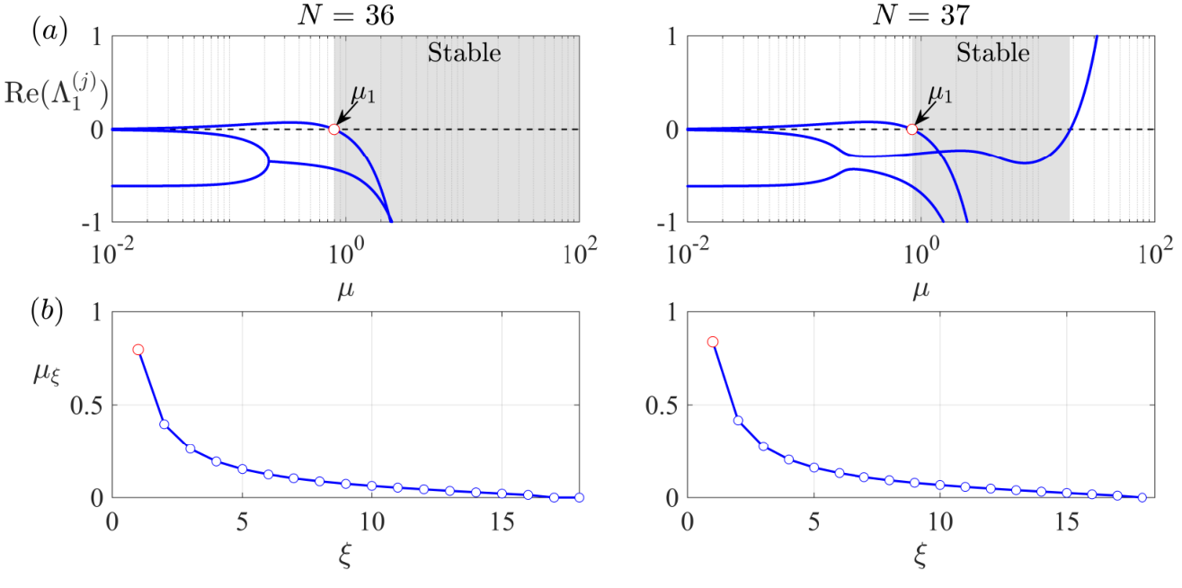
The eigenvalues, $\Lambda_{\xi}^{(j)}$ (for $j=1,2,3$), of $\text{M}_{\xi}(\mu)$ determine the stability of the spatially uniform state (21), where the dependence of $\Lambda_{\xi}^{(j)}$ on $\mu$ is presented in Figure 3. The onset of instability is determined by the eigenvalue (or one of a pair of complex-conjugate eigenvalues) of $\text{M}_{\xi}(\mu)$ with maximal real part; we denote this eigenvalue as $\Lambda_{\xi}(\mu)$ for each wavenumber, $\xi\in\{0,1,\ldots,N-1\}$. At a given value of $\mu>0$, the perturbed system (22) is neutrally stable if $\mathrm{Re}(\Lambda_{\xi}(\mu))\leq 0$ for all $\xi$, and unstable otherwise. We first note, however, that the rotational and temporal invariance of the spatially uniform state (21) implies that $\Lambda_{0}=0$ has multiplicity two. The remaining eigenvalue for $\xi=0$ is $-2\rho^{2}\text{Re}(\sigma_{2})=-2\text{Re}(\sigma_{1})<0$, corresponding to a stable perturbation from the periodic state for all $\mu>0$. Hence, if an instability to the periodic state arises, then it is for $\xi\neq 0$, corresponding to the emergence of a nontrivial spatial pattern. Moreover, for $\mu\gg 1$ and $\xi\neq 0$, the diagonal elements of the matrix $\mathrm{M}_{\xi}(\mu)$ dominate, from which we infer that the eigenvalues of $\mathrm{M}_{\xi}(\mu)$ are approximated by

$$\Lambda_{\xi}^{(1)}\sim\mu^{2}D_{2}\Delta_{\xi},\quad\Lambda_{\xi}^{(2)}\sim\mu^{2}(D_{1}\Delta_{\xi}-c_{g}\nabla_{\xi}),\quad\Lambda_{\xi}^{(3)}\sim\mu^{2}(D_{1}^{*}\Delta_{\xi}-c_{g}^{*}\nabla_{\xi}),$$

(24)

corresponding to advection and diffusion of perturbations. We recall that $\mathrm{Re}(D_{1})>0$, $D_{2}>0$, and $\Delta_{\xi}<0$ for $\xi\neq 0$. Hence, for $c_{g}=0$ (arising when $k_{c}=N/2$), all three eigenvalues have negative real part for $\mu\gg 1$ (as evidenced in Figure 3 for $N=36$). However, for $c_{g}\neq 0$, there are regimes in which the spatially uniform state is spuriously predicted to be unstable for $\mu\gg 1$ (a regime inconsistent with our $\mu=O(1)$ assumption), as presented in Figure 3 for $N=37$. To sidestep this spurious prediction, we therefore define $\mu_{\xi}>0$ as the largest value of $\mu$ at which $\text{Re}(\Lambda_{\xi}(\mu_{\xi}))=0$ and $\text{Re}(\Lambda_{\xi}(\mu))$ is a decreasing function of $\mu$ at $\mu=\mu_{\xi}$ (see Figure 3$(a)$ for reference). In the $\mu=O(1)$ regime of interest, the system is therefore unstable to perturbations for $\mu<\mu_{c}=\max_{\xi}\mu_{\xi}$.

A crucial feature of the system (9) is the coupling of the complex amplitude, $A_{n}$, with the mean, $B_{n}$, which acts to drive the instability of the spatially uniform state (21). We observe that variations in $B_{n}$ act as a source term in the amplitude, $A_{n}$, thus promoting spatial variations in $A_{n}$. For large $\mu$, the diffusion term in (9a) counteracts the growth of spatial variations of $A_{n}$, but this smoothing effect may become subdominant to the source term when $\mu$ is sufficiently small. Likewise, a similar competition between diffusion and the excitation of spatial variations in $B_{n}$ driven by variations in $A_{n}$ is apparent in equation (9b). As a consequence, this coupling provides a positive feedback loop for the emergence of spatial variations, whereas a BFN-like mechanism instead relies on sufficiently small dissipation. In fact, a true BFN instability only arises in the system (9) when the coupling coefficients, $\gamma_{i}$, and the group speed, $c_{g}$, vanish. A necessary condition for instability in this artificial case is $\text{Re}(\sigma_{2}D^{*}_{1})<0$ [15].

By numerically computing the eigenvalues of $\mathrm{M}_{\xi}(\mu)$, we observe that, similar to the BFN instability, the amplitude equations (9) exhibit a long-wave instability at $\xi=1$ (see Figure 3); hence, in the cases considered here, we have $\mu_{c}=\mu_{1}$. To capture this phenomenon analytically, we consider the special where $N$ is even and $k_{c}=N/2$, resulting in $c_{g}=0$ and $\gamma_{3}=0$. In this case, the spatially uniform state destabilizes via a real eigenvalue, for which the corresponding value of $\mu_{\xi}$ satisfies $\det\mathrm{M}_{\xi}(\mu_{\xi})=0$. This condition is satisfied by $\mu_{\xi}=0$ or when $\mu_{\xi}$ has a positive solution to

$$\Big[|D_{1}|^{2}D_{2}\Delta_{\xi}^{3}\Big]\mu_{\xi}^{4}-2\rho^{2}\Delta_{\xi}\Big[D_{2}\Delta_{\xi}\,\mathrm{Re}(\sigma_{2}D_{1}^{*})+\nabla_{\xi}^{2}\,\mathrm{Re}(\gamma_{1}^{*}\gamma_{2}D_{1})\Big]\mu_{\xi}^{2}-4\rho^{4}\nabla_{\xi}^{2}\,\mathrm{Im}(\sigma_{2}\gamma_{1}^{*})\,\mathrm{Im}(\gamma_{2})=0.$$

As $\nabla_{\xi}=-\nabla_{N-\xi}$ and $\Delta_{\xi}$ and $\Delta_{N-\xi}$, the coefficients of this equation are invariant under the mapping $\xi\rightarrow N-\xi$, so $\mu_{\xi}=\mu_{N-\xi}$ for all $\xi$. Moreover, to elucidate the dependence of $\mu_{\xi}$ on $\xi$, we consider the limiting case $\xi\alpha\ll 1$. In this limit, we observe that $\nabla_{\xi}^{2}\sim\Delta_{\xi}\sim-\xi^{2}$, yielding $\mu_{\xi}=\kappa\rho\sqrt{2}/\xi$, where $\kappa$ is a real and positive root of the quartic polynomial

$$P(\kappa)=\Big[|D_{1}|^{2}D_{2}\Big]\kappa^{4}+\Big[D_{2}\,\mathrm{Re}(\sigma_{2}D_{1}^{*})+\mathrm{Re}(\gamma_{1}^{*}\gamma_{2}D_{1})\Big]\kappa^{2}-\mathrm{Im}(\sigma_{2}\gamma_{1}^{*})\,\mathrm{Im}(\gamma_{2}).$$

If $P$ has a real and positive root then the form $\mu_{\xi}\sim\xi^{-1}$ suggests that the first wavenumber to destabilize is $\xi=1$ (or $\xi=N-1$, by symmetry); this long-wave instability is thus consistent with our slowly varying approximation of convolutions (see §2).

We proceed to explore the dependence of $\mu_{c}$ on the inter-droplet spacing, $\delta$, and spatial decay length, $l$, of the wave kernel, $\mathcal{H}$. Motivated by the form of the wave field arising in the bouncing-droplet system [24], a candidate wave kernel that satisfies the assumed periodicity, exponential decay and quasi-monochromaticity may be derived by projecting the form of the dimensionless radially symmetric wave $F(r)=\mathcal{A}J_{0}(2\pi r)\mathrm{sech}(r/l)$ onto a circle of circumference $2\pi r_{0}=N\delta$, where $r_{0}=R/\lambda$ [18]. Here $J_{0}$ is the Bessel function of the first kind with order zero and $\mathcal{A}$ is the amplitude of the wave. The resultant algebraic form of the wave kernel is

$$\mathcal{H}(x)=F\bigg(2r_{0}\sin\frac{x}{2r_{0}}\bigg),$$

(25)

where an example of this wave kernel is given in Figure 2$(b)$. For the numerical results presented herein, we consider $\mathcal{A}=0.1$ [18]. We note that the qualitative features of these results do not depend on the value of $\mathcal{A}$; increasing $\mathcal{A}$ simply serves to increase the amplitude of the wave field accompanying the equispaced lattice, the main consequence of which is a concomitant decrease in the critical memory, $M_{c}$.

References

- [1] I. S. Aranson and L. Kramer. The world of the complex Ginzburg–Landau equation. Reviews of Modern Physics, 74(1):99, 2002.
- [2] V. García-Morales and K. Krischer. The complex Ginzburg–Landau equation: an introduction. Contemporary Physics, 53(2):79–95, 2012.
- [3] M. C. Cross and P. C. Hohenberg. Pattern formation outside of equilibrium. Reviews of Modern Physics, 65(3):851, 1993.
- [4] A. C. Newell, T. Passot, and J. Lega. Order parameter equations for patterns. Annual Review of Fluid Mechanics, 25(1):399–453, 1993.
- [5] P. Coullet, L. Gil, and J. Lega. Defect-mediated turbulence. Physical Review Letters, 62(14):1619, 1989.
- [6] D. Tanaka and Y. Kuramoto. Complex Ginzburg-Landau equation with nonlocal coupling. Physical Review E, 68(2):026219, 2003.
- [7] V. García-Morales and K. Krischer. Nonlocal complex Ginzburg-Landau equation for electrochemical systems. Physical Review Letters, 100(5):054101, 2008.
- [8] J. Denk, L. Huber, E. Reithmann, and E. Frey. Active curved polymers form vortex patterns on membranes. Physical Review Letters, 116(17):178301, 2016.
- [9] T. H. Tan, J. Liu, P. W. Miller, M. Tekant, J. Dunkel, and N. Fakhri. Topological turbulence in the membrane of a living cell. Nature Physics, 16(6):657–662, 2020.
- [10] A. C. Newell and J. A. Whitehead. Finite bandwidth, finite amplitude convection. Journal of Fluid Mechanics, 38(2):279–303, 1969.
- [11] L. A. Segel. Distant side-walls cause slow amplitude modulation of cellular convection. Journal of Fluid Mechanics, 38(1):203–224, 1969.
- [12] M. C. Cross. Derivation of the amplitude equation at the Rayleigh–Bénard instability. Physics of Fluids, 23(9):1727–1731, 1980.
- [13] N. Stoop, R. Lagrange, D. Terwagne, P. M. Reis, and J. Dunkel. Curvature-induced symmetry breaking determines elastic surface patterns. Nature Materials, 14(3):337–342, 2015.
- [14] V. Hakim and W-J. Rappel. Dynamics of the globally coupled complex Ginzburg-Landau equation. Physical Review A, 46(12):R7347, 1992.
- [15] J. F. Ravoux, S. Le Dizes, and P. Le Gal. Stability analysis of plane wave solutions of the discrete Ginzburg-Landau equation. Physical Review E, 61(1):390, 2000.
- [16] K-I. Maruno, A. Ankiewicz, and N. Akhmediev. Exact localized and periodic solutions of the discrete complex Ginzburg–Landau equation. Optics Communications, 221(1-3):199–209, 2003.
- [17] S. J. Thomson, M. M. P. Couchman, and J. W. M. Bush. Collective vibrations of confined levitating droplets. Physical Review Fluids, 5:083601, Aug 2020.
- [18] S. J. Thomson, M. Durey, and R. R. Rosales. Collective vibrations of a hydrodynamic active lattice. Proceedings of the Royal Society A, 476(2239), 2020.
- [19] G. C Sethia and A. Sen. Chimera states: the existence criteria revisited. Physical Review Letters, 112(14):144101, 2014.
- [20] B. Thakur and A. Sen. Collective dynamics of globally delay-coupled complex Ginzburg-Landau oscillators. Chaos: an Interdisciplinary Journal of Nonlinear Science, 29(5):053104, 2019.
- [21] Y. Couder, S. Protiere, E. Fort, and A. Boudaoud. Walking and orbiting droplets. Nature, 437(7056):208–208, 2005.
- [22] J. W. M. Bush. Pilot-wave hydrodynamics. Annual Review of Fluid Mechanics, 47:269–292, 2015.
- [23] J. W. M. Bush, Y. Couder, T. Gilet, P. A. Milewski, and A. Nachbin. Introduction to focus issue on hydrodynamic quantum analogs. Chaos: an Interdisciplinary Journal of Nonlinear Science, 28(9):096001, 2018.
- [24] A. Eddi, E. Sultan, J. Moukhtar, E. Fort, M. Rossi, and Y. Couder. Information stored in Faraday waves: the origin of a path memory. Journal of Fluid Mechanics, 674:433–463, 2011.
- [25] J. Moláček and J. W. M. Bush. Drops walking on a vibrating bath: towards a hydrodynamic pilot-wave theory. Journal of Fluid Mechanics, 727:612–647, 2013.
- [26] C. Bechinger, R. Di Leonardo, H. Löwen, C. Reichhardt, G. Volpe, and G. Volpe. Active particles in complex and crowded environments. Reviews of Modern Physics, 88(4):045006, 2016.
- [27] C. Scholz, S. Jahanshahi, A. Ldov, and H. Löwen. Inertial delay of self-propelled particles. Nature Communications, 9(1):1–9, 2018.
- [28] M. X. Lim, A. Souslov, V. Vitelli, and H. M. Jaeger. Cluster formation by acoustic forces and active fluctuations in levitated granular matter. Nature Physics, 15(5):460–464, 2019.
- [29] H. Löwen. Inertial effects of self-propelled particles: From active Brownian to active Langevin motion. The Journal of Chemical Physics, 152(4):040901, 2020.
- [30] A. U. Oza, R. R. Rosales, and J. W. M. Bush. A trajectory equation for walking droplets: hydrodynamic pilot-wave theory. Journal of Fluid Mechanics, 737:552–570, 2013.
- [31] S. H. Strogatz. Nonlinear dynamics and chaos: with applications to physics, biology, chemistry, and engineering. CRC press, 2018.
- [32] J. K. Kevorkian and J. D. Cole. Multiple scale and singular perturbation methods, volume 114. Springer Science & Business Media, 2012.
- [33] C. R. Doering, J. D. Gibbon, D. D. Holm, and B. Nicolaenko. Low-dimensional behaviour in the complex Ginzburg-Landau equation. Nonlinearity, 1(2):279, 1988.
- [34] M. Bartuccelli, P. Constantin, C. R. Doering, J. D. Gibbon, and M. Gisselfält. On the possibility of soft and hard turbulence in the complex Ginzburg-Landau equation. Physica D: Nonlinear Phenomena, 44(3):421–444, 1990.
- [35] P. Coullet and S. Fauve. Propagative phase dynamics for systems with Galilean invariance. Physical Review Letters, 55(26):2857, 1985.
- [36] P. C. Matthews and S. M. Cox. Pattern formation with a conservation law. Nonlinearity, 13(4):1293, 2000.
- [37] N. L. Komarova and A. C. Newell. Nonlinear dynamics of sand banks and sand waves. Journal of Fluid Mechanics, 415:285–321, 2000.
- [38] S. M. Cox and P. C. Matthews. New instabilities in two-dimensional rotating convection and magnetoconvection. Physica D: Nonlinear Phenomena, 149(3):210–229, 2001.
- [39] T. B. Benjamin and J. E. Feir. The disintegration of wave trains on deep water. Journal of Fluid Mechanics, 27(3):417–430, 1967.
- [40] J. T. Stuart and R. C. DiPrima. The Eckhaus and Benjamin-Feir resonance mechanisms. Proceedings of the Royal Society of London. A: Mathematical and Physical Sciences, 362(1708):27–41, 1978.
- [41] P. A. Milewski and E. G. Tabak. A pseudospectral procedure for the solution of nonlinear wave equations with examples from free-surface flows. SIAM Journal on Scientific Computing, 21(3):1102–1114, 1999.
- [42] M. Durey, P. A. Milewski, and Z. Wang. Faraday pilot-wave dynamics in a circular corral. Journal of Fluid Mechanics, 891:A3, 2020.
- [43] D. M. Abrams and S. H. Strogatz. Chimera states for coupled oscillators. Physical Review Letters, 93(17):174102, 2004.
- [44] G. C. Sethia, A. Sen, and F. M. Atay. Clustered chimera states in delay-coupled oscillator systems. Physical Review Letters, 100(14):144102, 2008.
- [45] S. Nkomo, M. R. Tinsley, and K. Showalter. Chimera states in populations of nonlocally coupled chemical oscillators. Physical Review Letters, 110(24):244102, 2013.
- [46] E. A. Martens, S. Thutupalli, A. Fourrière, and O. Hallatschek. Chimera states in mechanical oscillator networks. Proceedings of the National Academy of Sciences, 110(26):10563–10567, 2013.
- [47] J. Wojewoda, K. Czolczynski, Y. Maistrenko, and T. Kapitaniak. The smallest chimera state for coupled pendula. Scientific Reports, 6(1):1–5, 2016.
- [48] J. F. Totz, J. Rode, M. R. Tinsley, K. Showalter, and H. Engel. Spiral wave chimera states in large populations of coupled chemical oscillators. Nature Physics, 14(3):282–285, 2018.