Learning to Optimise General TSP Instances
Abstract
The Travelling Salesman Problem (TSP) is a classical combinatorial optimisation problem. Deep learning has been successfully extended to meta-learning, where previous solving efforts assist in learning how to optimise future optimisation instances. In recent years, learning to optimise approaches have shown success in solving TSP problems. However, they focus on one type of TSP problem, namely ones where the points are uniformly distributed in Euclidean spaces and have issues in generalising to other embedding spaces, e.g., spherical distance spaces, and to TSP instances where the points are distributed in a non-uniform manner. An aim of learning to optimise is to train once and solve across a broad spectrum of (TSP) problems. Although supervised learning approaches have shown to achieve more optimal solutions than unsupervised approaches, they do require the generation of training data and running a solver to obtain solutions to learn from, which can be time-consuming and difficult to find reasonable solutions for harder TSP instances. Hence this paper introduces a new learning-based approach to solve a variety of different and common TSP problems that are trained on easier instances which are faster to train and are easier to obtain better solutions. We name this approach the non-Euclidean TSP network (NETSP-Net). The approach is evaluated on various TSP instances using the benchmark TSPLIB dataset and popular instance generator used in the literature. We performed extensive experiments that indicate our approach generalises across many types of instances and scales to instances that are larger than what was used during training.
Keywords Travelling Salesman Problem Deep Learning Learning to Optimise
1 Introduction
The Travelling salesman problem (TSP) is prevalent in combinatorial optimisation. It requires searching a set of given nodes, which can represent cities or places, to find a route that passes through each node exactly once and has minimal route/tour length. It has numerous applications in telecommunications, circuit board design, DNA sequencing, transportation and in theoretical computer science [1]. It is an NP-Hard problem, which means that there are instances for which finding an optimal solution is a time-taking process. Traditional approaches to tackle such hard optimisation problems employ two main strategies: exact algorithms [1], and heuristics [2]. Exact algorithms are based around enumeration and can solve TSP optimally, e.g., branch-and-bound or integer programming formulations, but they generally cannot scale to larger instances [1]. Since finding the optimal solutions might not be feasible for a large number of cities, heuristics employ problem-specific knowledge and carefully engineered approaches and parameters to find near-optimal solutions. Therefore, heuristics are effective algorithms which are often fast, but they may be tailored to a specific problem. Application of current search heuristics to new problems or extending to new instances of a similar problem is difficult and challenging. This challenge motivates the level of generalisation at which optimisation systems operate [3], and that is the underlying motivation behind learning to optimise algorithms to solve optimisation problems. Although existing approaches can find reasonable TSP solutions, they need to be restarted for every instance, even where similar instances have been solved before. Instead, the knowledge generated from solving previous instances can be reused and utilised using learning to optimise mechanism, and this can assist in initialising solutions for heuristic and exact solvers for improved and more efficient solution searching. We next describe some related work in learning to optimise area and the open challenges associated with them.
Deep neural networks (DNNs) have boosted performance in machine translation and image processing ([4]). In a similar way, deep learning architecture can be trained to predict solutions to many combinatorial optimisation problems. This new field is called Learning to Optimise [5]. Learning to Optimise approaches can be divided into supervised [6] and reinforcement learning-based [7], [8], [9], and have learnt to solve classic problems such as Travelling salesman [6], Knapsack [7] and Vehicle Routing problems [10]. In the supervised learning-based approaches, TSP instances and the corresponding ground truth solutions are used to train the DNN [6]. The reinforcement learning-based approach has been designed to solve combinatorial optimisation problems where policies are learnt to optimise tour length [7],[8],[9] and can be used as solvers. Although showing good initial promise, learning to optimise for COP suffers challenges.
- •
How to predict a solution for general TSP instances? For instance, TSP instances can be characterised by a) the space the points/cities are embedded in, e.g., Euclidean space and b) the difficulty of finding the optimal solution, which is partly related to how the points/cities are distributed within the space. We believe many of the existing approaches focus on training and testing on TSP instances that are embedded in Euclidean space. Also, they focus on generating training and testing instances that are uniformly distributed within a unit hypercube. This can lead to an inability to model, learn on and generalise to TSP instances that are embedded in non-Euclidean spaces and points (nodes) are not uniformly distributed.
- •
How to generate appropriate training data to be able to learn to solve different instances of TSP adequately? Though it is difficult to generate training data using various TSP instances, however, it is easy to generate Euclidean TSP instances/easy instances that we can use as training data to solve all types of TSP instances and easy to find optimal solutions (for small size ) of some Euclidean TSP instances using Concorde [11]. Therefore, we consider generating Euclidean TSP instances as training data that are easy to generate and find a solution and predict solutions for any types of instances.
The motivation of this paper is to present an approach that can able to solve general (various size and difficulty level) TSP instances, given the greater availability of Euclidean instances considering the above mention challenge. We next describe the various size and difficulty level of TSP instances that never analysed before in learning to optimise area in the next two paragraphs.
Studies have been shown that the main property of measure the difficulty of TSP problem related to how the cities are distributed (and the distance space). In [12] studied all the TSP instances do not have the same difficulty level such as difficulty/distribution of points (easy, hard and so on) and in terms of size (instance size). We illustrate two examples of TSP instances, for example, hard (Berlin52) and easy(TSP50). In Fig. 1(a), Berlin52 is an example of a hard problem because of the tightly constrained points; it is hard to search solutions that made the problem hard. In Fig. 1(b), TSP50 is an example of an easy problem as the points are loosely constrained, so it is easy to search for solutions for these problems. Hardness generally relates to the distribution of the normalised areas and the distances between the cities. For example, the number of cities, represented as a dot(.) in Fig. 1], spread in the area covered by the cities of the given problem. This distribution of the cities represent how instances are embedded in the space, and how hard or easy an instance is to solve, as described in [13]. In [13], they classified TSP instances according to their hardness such as easy, and hard to solve instances. In Fig. 1(c) and 1(d) is the solution for Fig. 1(a) and 1(b) where we illustrate that although instance size is nearly the same for two problems according to distributions of the problems, the solutions also alter on how the number of cities spread in the place. We define hardness indication details in Section 3.3. In this paper, motivation is not to measure the difficulty level of TSP instance, but, we are using the measure to show our model can learn all types of instances (hard and easy) studied in [13], which is verified in Section 5.3.1.
Another types of TSP instances embedded non-uniform manner with various edge-weight types illustrates in Fig. 2. Edge is a property of new measure of the city to city nearness. Every TSP instances can be classified as their edge-weight types (weight means distances), such as Euclidean distance, Haversine distance11 1 The edge weights represent the geographic distances (Haversine) between these locations, and TSP points are distributed on a sphere considering the curvature of the Earth., pseudo-Euclidean distance22 2 Pseudo-Euclidean instances, which is Euclidean distance but breakdown of some properties of Euclidean space since the triangular inequality is not satisfied [14]. In Fig. 2, we illustrate that every edge-weight type of TSP instance embedded differently in the space, which formulates in Section 3.2. These instances never analysed before in learning to optimise area. Previous work by the author has evaluated using Euclidean distance TSP instances, and it is anticipated that evaluate other distance types of TSP instances is preferred. Consequently, since we are considering learning general TSP instances so from the TSPLIB library [15], we observe various edge-weight types of instances to evaluate our model. We showed our model able to generalise on the different types of common TSP problems that we want one learning algorithm to generalise over, and that existing works have difficulty in generalising. Subsequently, we show the competitiveness of our approach.


In real-world TSP applications, the instances consists of hundreds or thousands of nodes with various structures, and the optimal solution is not able to compute efficiently. We find that the proposed NETSP model generalises well from small-scale TSP problems to larger-scale problems and the various structure of distribution of the problems (cities) and generalisation capacity increases by order of magnitude. Cities may be distributed in a structured or unstructured way, which makes each TSP problem hard [16], [13]. We present a new approach to solve the TSPs embedded in different spaces, and consider the distribution of points, also study different difficulty level of instances [13]. Subsequently, different edge-weight types [17] of instances from the TSPLIB benchmark dataset [18] and classify them according to their edge-weight types and hardness. Moreover, we presented that we trained our model with smaller instances but can generalised larger instances. This paper introduces a deep learning approach using a combination of Convolution Neural Network (CNN) [19] and Recurrent Neural Network (RNN) [20]. CNN has been successfully shown to be able to handle different embedding spaces, and as we show in this paper, it is also able to handle TSPs in different spaces. Also, a CNN architecture can discover the inherent micro-patterns within smaller instances that transfer to larger instances and different spaces. In the field of combinatorial optimisation research, we have proposed the Non-Euclidean travelling salesman problem architecture (NETSP-Net) in Fig. 4, which aims to learn various TSP instance representations and capture important features (such as local spatial patterns among coordinates to learn about the pattern between two nodes). The objective of this work is not to outperform the current state-of-the-art TSP learning algorithm but to motivate the research in supervised learning to learn general TSP instances, considering the above difficulties.
The main contributions of our work are as follows:
- •
We propose a new architecture, that we call NETSP-Net whose model is applied to non-trivial algorithmic problems involving geometry in various travelling salesman problems.
- •
Our NETSP-Net is applied to different distributions of TSP instances embedded in the Euclidean plane (hard to solve instances). We show that the learned model generalises to various distributions.
- •
We show that our method can generalise on various TSP instances embedded in various spaces.
- •
We show that our supervised model is efficient compared to reinforcement learning and can generalise to larger problems and perform consistently compared to other learning models.
2 Related work
Before presenting NETSP-Net, we review some background that is related to our model. Over the last few years, much work has been done to tackle combinatorial optimisation problems, particularly from a learning perspective. To begin with, we discuss exact and heuristic solutions, followed by learning algorithms for TSP as well as policy-based methods.
2.1 Exact and heuristic solvers
Combinatorial optimisation problems intensely studied in the operation research field is the travelling salesman problems (TSP). Many algorithms such as exact, heuristics and meta-heuristic can provide the approximate solutions efficiently for larger problems. The exact algorithms (TSP solver Concorde [1]) can find solution optimally. However, for solving larger problems, the algorithms become slower, and there is an exponential increase in the execution time [21]. In practice, many heuristic approaches are employed including swarm optimisation, simulated annealing, local search, genetic and greedy algorithms[22]. The approximate search heuristic for the symmetric TSP the Lin-Kernighan-Helsgaun heuristic [23], has been shown to solve instances with larger problems optimally. OR-Tools (developed by Google) [24] is a solver for vehicle routing problem, tackles the TSP with a combination of local search algorithms and meta-heuristics. Substantially, these approaches need expertise and require extensive problem-specific research.
2.2 Sequence to sequence learning on Neural Combinatorial Optimisation
Recent advances in the neural networks include the design of a new model architecture called Pointer Network(PN) [6], inspired by sequence-to-sequence models where the input sequence can determine the output sequence. In sequence-to-sequence models, the overall architecture requires two RNN networks referred to as an encoder-decoder framework. An encoder network receives the input sequence (source information) and encodes the source information into a vector representation. Later, a decoder generates an output sequence from this. In the Sequence-to-Sequence architecture, the encoder takes the input sequence and generates the output sequence based on one vector. For example, [25] demonstrates that during decoding steps, using a technique name attention mechanism the decoder can extract important parts of the source information (input sequence) and produces the output sequences using the corresponding information.
2.2.1 Neural Combinatorial Optimisation using Supervised Learning Techniques
Pointer Network(PN) [6] learns to solve combinatorial optimisation problems where encoder(RNN) converts the input sequence that is fed to the decoder(RNN). They use attention on the input sequence and trained the model to solve the Euclidean TSP. The PN architecture has been developed to solve TSP, they trained their network using a supervised method (training date is the randomly generated problem instances with their ground truth optimal (or heuristic) solutions). In [26] takes a graph as an input and used several graph convolutional layers to extract features from its (graph) nodes and edges. The output of the neural network is an adjacency matrix whose elements represented the probabilities of edges. The edge predictions are then transformed into a feasible tour. Joshi et al. [26] also trained the model in a supervised manner.
2.2.2 Neural Combinatorial Optimisation using Reinforcement Learning Techniques
In recent years, researchers develop reinforcement learning-based frameworks to solve TSP problems [7], [8], [27], [9]. The proposed model called EAN [8] used Principal Component Analysis (PCA) on the input coordinates. They do not use any recurrent and convolutional layer instead used attention mechanisms [28], moreover first time they combine 2OPT local search with improving performance. Model names S2VDQN [27] used a graph embedding structure first in the combinatorial optimisation field. They trained the model using the reinforcement learning deep Q-network (DQN) to develop solutions for graph-based NP-hard problems incrementally. The framework proposed by Kool et al. [9], based on deep reinforcement learning that utilized graph attention layers, demonstrated that high-quality approximate solutions can be achievable to some NP-hard COPs. In [9], construct a solution for TSP by pointing input elements as a sequence. They claim their model is an alternative to the PN [6]. Another recent method called (GNN-MCTS), a graph neural network (GNN) [29] used Monte Carlo Tree Search (MCTS) to make the decision more reliable by simulating a large number of searches. GNN [29] is trained to guide the MCTS, which helps to reduce the complexity of the search space. Also, to avoid stuck in a local optimum MCTS provides a more reliable policy [30].
In the learning to optimisation field, previous work only considered the TSP instances embedded in a Euclidean plane and randomly generated TSP instances. Our goal is to consider TSP instances according to their edge weight types and distribution. Our model is based on a CNN combined with RNN and attention mechanisms, and this combination significantly improves results. In our work, we have used a CNN, which is more powerful to exploit spatial invariance of all locations (cities). The hardness of TSP instances have been investigated many times [12],[31] and solve various edge-weight types [32] of TSP instances in the operation research field. However, in the learning to optimise field, never address the issue of the hardness of TSP instances and other edge-weight types of instances from the TSPLIB benchmark dataset [18]. We show the benefit of our model in direct comparison to state-of-the-art approaches using randomly generated data, as well as TSPLIB data on various TSP instances.
3 Background and Problem Formulation
In this section, we formally define the problem. We first present the TSP problem, then define what learning to optimise means when solving TSP instances.
3.1 Travelling Salesman Problem (TSP)
In the TSP problem, we are given a set of points/cities33 3 We will use cities and points inter-changeably to mean the same thing. , embedded in a d-dimensional space, i.e., and . For routing and navigation, it is typically d = 2, i.e., , but we stress TSP and our approach can handle problems of any dimensions. Let, D (), denote a distance measure between cities and , i.e., . D can be the Euclidean distance, but can also be other distances which we will shortly introduce. A tour of these cities is a sequence where each city is visited, and only visited once. Let a tour be denoted by where each and . Then the TSP problem is to find such a tour of cities such that the total travel distance between consecutive pairs of cities in the tour is minimised:
3.2 Popular TSP Distance Measures
In this section we introduce and formally define popular distance measures used for TSP. These include Euclidean distance, Haversine instances, pseudo-Euclidean instances.
3.2.1 EUC2D
The Euclidean distance is a popular and commonly used metric to compute distance. It is defined as [17]:
where denotes the value of the dimension of point/city .
3.2.2 Haversine distance
The Haversine distance [33] was introduced to correct and take account of the curvature of the Earth, and a popular distance for navigation and solving TSP where points are distributed on a sphere. The haversine formula determines the great-circle distance between two points on a sphere. It typically defined in terms of latitude and longitude, so consider the case where our cities are described by two dimensions, latitude and longitude,(both in radius). Haversine is important in navigation that relates the sides and angles of spherical triangles. In Fig. 2(a), shows a geographic TSP instance with 16 vertices, name ’ulysses16’ 44 4 The distance matrix for this instances was computed using the Haversine formula (great circle distance) [34], that is, the shortest round trip. This route is calculated based on direct air distances and can only be travelled by a ’modern Ulysses’ using an aircraft. The solid line and arrows indicate the sequence in which Homer’s Ulysses supposedly visited the 16 locations. The Haversine distance is thus defined as follows [17]:
where is latitude, is longitude and is the radius of the sphere over which the distance is computed, e.g., the radius of Earth.


3.2.3 Pseudo-Euclidean
The instance, ATT48, indicates the edge weight type used is pseudo-Euclidean [15]. The instance, ATT48, represents the 48 capitals of the adjacent mainland U.S. states and ATT specifies the edge weight type used is pseudo-Euclidean [35]. Pseudo-Euclidean [15] is a Cartesian product of two Euclidean spaces with a specific inner product and the distance. The Pseudo-Euclidean space (PE-space) consists of two orthogonal Euclidean sub-spaces, called the positive space and the negative space. Pseudo-Euclidean is not a metric space as it does satisfy the triangular inequality 55 5 The pseudo-Euclidean space geometry has a breakdown of some properties of Euclidean space. In particular it is not a metric space [15]. For vectors and in a real affine space, there exists a definite number, called the scalar product (a,b). In Pseudo-Euclidean space, there are three types of straight lines: Euclidean, ((a, a)¿0), pseudo-Euclidean ((a, a)¡0) and isotropic ((a, a)=0). Isotropic cone represents the merging of all the isotropic straight lines passing through a point. Furthermore, there are several types of space in a pseudo-Euclidean space, such as Euclidean, pseudo-Euclidean and semi-Euclidean (spaces containing isotropic vectors). This means pseudo-Euclidean space also can be understood as Euclidean space.. The distance is calculated by finding the difference between co-ordinates of the cities and summing the square of these differences, dividing by ten and calculating the square root. It is defined as [14]:
where denotes the value of the dimension of point/city .
In Fig. 2(b), shows a TSP (pseudo-Euclidean space) instance with 48 vertices, name ’att48’ and edge represent how cities are connected. So, we motivate to use Att48 instance and haversine instance, which can be considered as non-Euclidean TSP instances, which is different from Euclidean distance instances.

3.3 Measure the Difficulty Level
In [36], the authors suggested that the hardness of solving the travelling salesman problem is related to how the cities cover the area and spread across the area (space). They analysed how easy and hard a TSP instance to find a new solution with a shorter tour length. To the effort, authors place this phase transition at , where N is the number of cities, A the area covered by the cities and l the tour length. They set a parameter which can be used as hardness indicator, that measure the difficulty to solve a TSP instance. In [13] they argued that this measurement requires finding the optimal or a quasi-optimal solution of the instance which makes this calculation difficult to use this measure frequently. Therefore their finding is the hardness of TSP instances based on spatial properties of instances such as space and distribution of cities. In [13], given the parameters, A and N, the decision problem becomes more difficult for instances with . Therefore, the closeness of to 0.75 can provide an additional hardness rank for comparison purposes, and illustrate an example of the most difficult instance Berlin52.
3.4 Learning to Optimise TSP
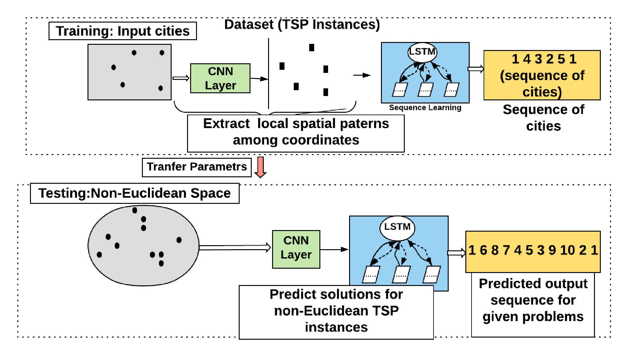
In (supervised) learning problems, we generally map inputs to outputs given a training dataset of examples (input, output). (Supervised) Learning to optimise similarly does this mapping and learning, but the inputs are optimisation problems and outputs are their solutions. During training, the learning model learns to map input instances to TSP solutions, then during testing/prediction phase, a solution is predicted for each input instance. This is summarised in Fig. 3.
More formally, given a set of training examples , a learning algorithm searches for a function, , where is the optimisation instance/problem space and the solution space . Alternatively and equivalently, we want to find a Y solution that minimises the optimality gap. For learning to optimise, we just obtain that mapping function differently to optimisation.
4 Proposed Model: NETSP-Net
Our approach, the Non-Euclidean TSP network (NETSP-net) comprises CNN with two RNN modules with attention mechanism [6] The employed encoder and decoder both consists of Long Short-Term Memory (LSTM) cell [20]. The reason we use LSTM, because, it is difficult for RNNs to handle long-term dependencies in the input sequence, LSTM capable of learning long-term dependencies. We are inspired by previous work [6] that used a set of softmax layers, and the overall model is illustrated in Fig. 4. This approach allows the model to effectively focus on a specific position in the input sequence rather than predicting an index value. We employ the attention mechanism architecture, depicted in Fig. 5, where the encoder produces embedding of all input nodes, then fed to the decoder network (green). The decoder produces the sequence S as a solution (TSP tour). Our model uses CNN for the representation of inputs to exploit the spatial invariance of all nodes (cities), as this technique can discover the micro-patterns of TSP instances. Our particular choice of CNN to generalise to unseen various TSP instances such as Non-Euclidean TSP instances. Thus, 1-Dimensional convolutional layers use as an embedding that maps the inputs into D-dimensional vector space, then the elements are fed as an input to the RNN. The first RNN network reads the embedded inputs and uses another LSTM layer to produce or decode the output of S. In the next section, describe the details of each part.
4.1 Architectural Details
In this section, we formally define our NETSP-Net model in terms of TSP. Given a problem instance C, represented as a sequence of n cities in a two-dimensional space, where node . We are interested in finding a minimised tour S, where each city is visited once with a minimum total length. In Fig. 7, for TSP we find an illustration of an input/output pair (C,S). This dominant approach inspired by sequence to sequence model is based on learning general TSP instances, which optimising (training) for the likelihood of the next target city conditioning on the input sequence and the ground truth TSP tour. In the sequence to sequence model, given a training pair, , it computes the conditional probability , (see in Fig. 5), estimate the terms of the probability chain rule using a parametric model, i.e.,
| (1) |
Where is the sequence of cities, and is its correct solution. By maximising the conditional probability for the training dataset, the parameters of the model are learnt, and using the following formulation, where the sum is an over the training example:
| (2) |

Encoder: For the encoder, we use 1-dimensional convolutional layers. Unlike languages, when there is no meaningful order in the input, such as TSP, use CNN will be more effective. For example, the inputs are the set of unordered locations (nodes) in the TSP, and any random order holds the same information as the initial inputs. Therefore, in our model, we improve the encoder by directly using the embedded inputs from 1-dimensional convolutional layers. Illustrates in Fig. 6, shows while Conv1d scanning over the coordinates of the cities, it can extract the compositional features, for example looping through the existing ones and draw attention to the repeated patterns to discover geometry involved in the instances from the inputs 66 6 In general, 1D convolutional mechanism, information flows by a convolution operation () followed by an activation function, , where C and K denotes the incoming input signal and a kernel respectively. We illustrated in Section 5.3.3 to show our claim that embedding layer always gives a better solution (One possible explanation is that the model efficiently extracted the useful features from the high-dimensional input representations). Here, used embedding layer (CONV1D), in which the in-width is equal to the input length, the number of the filter is F which covers how many different windows from the input is considered. The number of in-channels is the number of elements of C. Input nodes is embedded and processed by CNN layer. From the -dimensional input features , the encoder computes initial -dimensional node embeddings (we use ). Subsequently, the RNN layer in encoder reads the embeddings and generates the latent memory states , where . At time-step , the input to the RNN network is a d-dimensional embedding of a 2D point , which is obtained via a linear transformation of shared across all input steps, Fig. 5. We use a 1-dimensional convolutional network here since the 2-dimensional convolutional does not lead to significant improvement in our experiments. In the next section describes decoder networks.

Decoder:
The decoder network uses an attention mechanism (followed by pointer network attention technique) to produce a distribution over the next city to visit in the tour and generates the latent memory states where and, at each step i. Then to the next decoder step decoder receives the next selected city. The first decoder step input (denoted by in Fig. 5) is a d-dimensional vector treated as trainable parameters of our NETSP-Net. During inference, given a sequence C, the learnt parameters select the sequence S with the highest probability of good solutions. (C, S) is the training example pair, and we utilised stochastic gradient descent to optimise the sum of the log probabilities over the training set. Further training details are given in subsection 5.2.
Attention mechanism: We now describe our attention mechanism. In Fig. 5 demonstrates the attention mechanism [7] employed in our model, that, we utilise this to extracts the related information from the inputs. Our attention mechanism, takes input as a query as a vector and a set of reference vectors where , and predicts a distribution over the set of k references. This probability distribution represents the extent to which the model points to the reference for the query q. The description of our attention function can be found in Appendix A. Some additional computation steps, named glimpses, suggested in [6] is used that aggregates the contributions of different parts of the input sequence, like [25]. The details of this approach is discussed in Appendix A.

5 Experiments
In this section, we discuss the experiment setting for the proposed method. First, the model is evaluated using various TSP instances according to their hardness and use one large instance from TSPLIB library to show that model can generalise on large scale TSP instances in Table 1. Second, we consider the non-Euclidean TSP instances, such as Pseudo-Euclidean instances, Geographical (Haversine distance) instances in Fig. 9. Moreover, we compare the performance of our model on random TSP instances as previous state of the art approaches typically focus TSP random data, reported in Table 2. We investigated the behaviour of the proposed NETSP-Net approach and compared with other baselines. Our experiments were designed to investigate the following evaluation procedure:
- •
We explore the performance of our model on easy, and hard TSP instances.
- •
In order to verify the generalisation of the proposed method, we test our method on the various edge-weight types of TSP instance.
- •
The performance of our method is evaluated on randomly generated instances that previous work concentrated on.
- •
Analyse model performance using various training and testing size and the result shown.
- •
- •
Compare the solution quality of 1-dimensional convolutional network with 2-dimensional convolutional networks in Appendix D.
In the rest of this section, we discuss our dataset, network settings, baselines we compared and finally present our results.
5.1 Datasets
To evaluate our model, we have used the benchmark TSPLIB dataset [18] (different edge-weight types of TSP instances) and randomly generated instances; dataset was first introduced by [6]. The TSPLIB is a popular benchmark for evaluating TSP algorithms. For the synthetic data, we follow [6] and generate TSP instance by generating points in within a 2D unit square , uniformly randomly. The test datasets have graphs of sizes 20, 50 and 100 nodes. The training sets consist of one million pairs of problem instances and solutions. The test sets consists of 1000 pairs each.
5.2 Network Setting
We used the same architecture settings throughout all the experiments and datasets. In all our experiments, use mini-batches of 128 sequences, one-dimensional convolutional operation, convolution layer works as an embedding layer which embed each city location is into a vector of size 128, LSTM cells with 128 hidden units and we train our models with the Adam optimiser [38]. For the randomly generated dataset, we use an initial learning rate of 0.001 (considered best learning rate) for TSP20, TSP50, TSP100. The decay rate of every 5000 steps by a factor of 0.96. We clip the L2 norm of our gradients to 1.0. We varied the hyper-parameters and found results are most similar. Run times are important but can vary due to implementation using Python or C++. We used python for implementation. Another important factor is using hardware such as GPUs or CPUs [9]. We implemented our experiments on the same hardware platform with Intel Xeon 2.4 GHz with 56 cores. We run Concorde [11] and OR-Tools [24] on Intel i5-7200U CPU@2.50 GHz as we do not show run times in our evaluation, used different hardware.
5.2.1 Evaluation
5.2.2 Baselines:
The performance of our technique compared with a variety of baselines, including: Solvers, an efficient exact solver specialized for TSP; heuristics, well-known heuristic solvers that achieves state-of-the-art performance on various routing problems; open source software for combinatorial optimisation (OR-Tools), a mature and widely used solver for routing problems based on meta-heuristics; learning models using supervised techniques(SL); and learning methods using reinforcement learning (RL). We report optimal results by Concorde specialized for TSP [11]. We compare against 2-opt and Christofied local search, MST, Cheapest, Nearest, Random and Farthest Insertion, as well as Nearest Neighbor in Table 1 and 2. We also focus our comparison to the recently proposed deep learning methods [6], [26], [7],[8], [27], [10] and [9] using their publicly released implementations in Table 2. We also compared our results with Google Or-Tools [24] in both the tables 1 and 2. The description of baselines, experimental procedures are as follows:
| Easy=>Hard | Opt | Furthest | 2opt | Christ | Cheapest | MST | Or | AM | S2V-DQN | NETSP |
| Eil51 | 426 | 567 | 446 | 527 | 494 | 614 | 427 | 435 | 439 | 427 |
| Eil76 | 538 | 583 | 591 | 646 | 607 | 743 | 538 | 564 | 564 | 543 |
| Eil101 | 629 | 659 | 702 | 728 | 693 | 847 | 651 | 668 | 659 | 632 |
| St70 | 675 | 712 | 753 | 836 | 776 | 858 | 682 | 829 | 696 | 712 |
| Ch150 | 6,528 | 7,210 | 7,232 | 7,641 | 7,995 | 9,203 | 6632 | 9298 | 6985 | 6870 |
| Ch130 | 6,110 | 6,498 | 6,470 | 7,367 | 7,279 | 8,280 | 6147 | 6329 | 6270 | 6133 |
| Berlin52 | 7,542 | 8,307 | 7,788 | 8,822 | 9,013 | 10,402 | 7542 | 7788 | 7542 | 7542 |

- •
Concorde: Concorde also denoted as (OPT) in Table 1 is a computer code for the symmetric TSP and some related network optimisation problems. Concorde’s TSP solver has been used to obtain the optimal solutions for all random instances and TSPLIB instances; We implemented Concorde [11] that use algorithms [39, 40, 41]. In Table 1 and Fig. 8 denoted the results as OPT. In Fig. 9 denoted the result as optimal.
- •
Nearest Insertion: Nearest Insertion [42] inserts the node to the nearest set of nodes (neighbours), for such insertion operation causes the least cost in the overall tour length.
- •
Farthest Insertion: Furthest Insertion [42] needs to select two cities and connect them to get the least cost tour, then find another farthest city of this tour. Repeat the step until every city associates to complete the tour
- •
Random Insertion: Random Insertion [43] needs to select two cities. A Random insertion adds a random node where the added node order is also random similar to the nearest neighbour.
- •
Nearest neighbour: The Nearest Neighbour [42] heuristic represents the partial solution as a path with a start and end node. First, start in some city and the select to visit the city to the starting city. Continue the process, and at the end, all cities visited, and the end city is connected with the start city. We follow the implementation of [9].
- •
2-Opt: Croes [44] first introduced the 2-optimisation method, which is a simple and very common operator. The idea of 2-opt is to exchange the links between two pairs of subsequent nodes.
- •
Minimum Spanning Tree: A Minimum Spanning Tree (MST) [45] aims to minimise the weights (tour lengths) of the edges of the tree.
- •
Christofides: Christofides algorithm [2] is a heuristic algorithm which aims to find a near-optimal solution to the problem. It follows steps, first find an MST (minimum spanning tree ), second find a minimum-weight perfect matching M among vertices with odd degree. Create a minimum spanning tree T of G, to Make a multigraph G; it combines the edges of M and T. Then find an Euler cycle in G by skipping vertices already visited.
- •
Cheapest: The Cheapest-Link Algorithm select the edge with the smallest weight and mark it and continue that following rules, do not pick an edge that will close a circuit –Do not pick an edge that will create three edges coming out from a single vertex Connect the last two vertices to close the circuit.
- •
OR-Tools: Google Optimisation Tools (OR-Tools) is an open-source solver for combinatorial optimisation problems. OR-Tools contains one of the best available vehicle routing problem (VRP), which is a generalisation of the TSP and implemented many heuristics for finding an initial solution and metaheuristics, we use it as our baseline. We have used the local-search meta-heuristics used in OR-Tools as Guided Local Search.
- •
Pointer Network(PN): We implemented the pointer network with supervised learning [6]
- •
- •
EAN: For experiment Policy gradient across all tasks, we follow the configuration provided in ([8]), and we report results.
- •
[ and ]: For experiment, Nazari et al. ([10]) implemented following the GitHub code 77 7 https://github.com/OptMLGroup/VRP-RL.
- •
: For experiment, ([9]), initiating parameter uniform , with the input dimension. Every epoch we process 2500 batches of 512 instances. Used a constant learning rate 0.0001 Training with a higher learning rate 0.001 is possible and speeds up initial learning, but requires decay (0:96 per epoch) to converge. Implemented following the the GitHub code 88 8 https://github.com/wouterkool/attention-learn-to-route.

5.3 Results
In this section, we compare the solutions produced by proposed and baselines methods mentioned in Section 5.2.2.
| Method | TSP=20 | TSP=50 | TSP=100 | ||||
|---|---|---|---|---|---|---|---|
| Solver | TourL | Gap | TourL | Gap | TourL | Gap | |
| Concorde | 3.84 | 0.00% | 5.70 | 0.00% | 7.77 | 0.00% | |
| Heuristics | |||||||
| Nearest Neighbour | 4.50 | 17.18% | 7.00 | 22.80% | 9.68 | 24.58% | |
| Nearest Insertion | 4.33 | 12.76% | 6.78 | 18.94% | 9.45 | 21.62% | |
| Random Insertion | 4.00 | 4.16% | 6.13 | 7.54% | 8.51 | 9.52% | |
| Farthest Insertion | 3.92 | 2.08% | 6.01 | 5.43% | 8.35 | 7.46% | |
| Meta-heuristic | |||||||
| Or-tools | 3.85 | 0.26% | 5.80 | 1.75% | 8.30 | 2.90% | |
| Learning Models (SL) | |||||||
| PN [6] | 3.88 | 1.03% | 6.62 | 16.14% | 10.88 | 40.20% | |
| GCN* [26] | 3.86 | 0.52% | 5.87 | 2.98% | 8.41 | 8.23% | |
| Learning Models (RL) | |||||||
| Bello et al.[7] | 3.89 | 1.30% | 5.99 | 5.08% | 9.68 | 24.73% | |
| EAN. [8] | 3.93 | 2.34% | 6.63 | 16.31% | 9.97 | 28.31% | |
| S2vDQN* [27] | 3.89 | 0.26% | 5.99 | 1.75% | 8.31 | 7.07% | |
| RL+Gr[10] | 4.00 | 4.16% | 7.01 | 22.98% | 9.46 | 21.75% | |
| RL+BS[10] | 3.96 | 3.12% | 7.40 | 28.82% | 8.93 | 14.92% | |
| AM+Gr[9] | 3.87 | 0.78% | 5.80 | 1.75% | 8.15 | 4.89% | |
| NETSP-Net (Ours) | 3.85 | 0.26% | 5.85 | 2.63% | 8.31 | 6.94% | |
5.3.1 Generalisation on Different Distributions and Larger Instances
In this section, our target is to investigate our model’s performance on different distribution. We use the standard TSPLIB library [18], which is publicly available. We show that the model generalises reasonably well to large problems and a very different distribution. Moreover, the model was trained on instances with no more than cities. We classify TSP instances by how they are distributed on the Euclidean plane, which indicates the hardness of the instances. Note that these instances may follow distributions that are completely different from those used in training, e.g., in node location patterns. In Table 1, we have reported the optimal TSP solutions implemented using Concorde [1], then compare against other learning methods AM, [9] (using their publicly available code using benchmark TSPLIB dataset, trained using random data) and S2V-DQN [27] (reported their result). Furthermore, compare against other heuristics, e.g., Furthest, 2-opt, Christofides, Cheapest, MST and OR-tools [24]. Also, we arrange the instances from easy to hard (in the first row is the easy instance, and the last row is the hardest instances). It is clear that the structure of TSP instances influences the solution quality, which our model able to understand and shows that our approach performs relatively well on these instances. Table 1 demonstrates that our model performs well on the various hardness of TSP instances when compared to other two learning algorithms [27] and [9], which means the model can generalise beyond random data (benchmark data). We show that the quality of our solution does not degrade very fast with the increase of problem size, but other approaches lost performance progressively faster for larger problem sizes in Table 1 and in Fig. 8. For larger problem size, we wanted to know, what extent the learned algorithm generalises to larger problem sizes. In Fig. 8, we illustrate the most larger problems A280 data (from TSPLIB data) learned by our model. It compares the gap to the optimal solution, with a smaller gap been more desirable. The optimal solutions (opt) are obtained from the Concorde algorithm. We observed that for large-scale TSP instances, the NETSP-Net outperforms both state-of-the-art learning approaches [27] and [9], which demonstrates the usefulness of our approach. The convolutional neural network has shown to be powerful to represent the spatial patterns among coordinates. Embedding with a convolutional network increases the learning efficiency and generalises to larger problems resulting in predicted solutions for various TSP instances.
| Method | Training Size | Testing Size | TourL | |||
|---|---|---|---|---|---|---|
| Problem | Size | Problem | Size | TourL | Gap | |
| Learning Models (RL) | ||||||
| AM.[9] | TSP | 20 | TSP | 20 | 3.85 | 0.26% |
| AM.[9] | TSP | 20 | TSP | 50 | 5.95 | 4.38% |
| AM.[9] | TSP | 20 | TSP | 100 | 9.18 | 18.14% |
| AM.[9] | TSP | 50 | TSP | 20 | 3.87 | 0.78% |
| AM.[9] | TSP | 50 | TSP | 50 | 5.80 | 1.75% |
| AM.[9] | TSP | 50 | TSP | 100 | 8.15 | 4.89% |
| AM.[9] | TSP | 100 | TSP | 20 | 4.14 | 7.81% |
| AM.[9] | TSP | 100 | TSP | 50 | 5.94 | 4.21% |
| AM.[9] | TSP | 100 | TSP | 100 | 8.12 | 4.50% |
| Learning Models (Ours) | ||||||
| NETSP-Net | TSP | 20 | TSP | 20 | 3.85 | 0.26% |
| NETSP-Net | TSP | 20 | TSP | 50 | 5.81 | 1.92% |
| NETSP-Net | TSP | 20 | TSP | 100 | 9.01 | 15.95% |
| NETSP-Net | TSP | 50 | TSP | 20 | 3.85 | 0.26% |
| NETSP-Net | TSP | 50 | TSP | 50 | 5.85 | 2.63% |
| NETSP-Net | TSP | 50 | TSP | 100 | 8.31 | 6.94% |
| NETSP-Net | TSP | 100 | TSP | 20 | 3.86 | 0.52% |
| NETSP-Net | TSP | 100 | TSP | 50 | 5.87 | 2.98% |
| NETSP-Net | TSP | 100 | TSP | 100 | 8.30 | 2.90% |
5.3.2 Generalisation on NON-Euclidean TSP Instances
In this analysis, we show the results of evaluating the different edge-weight types from the TSPLIB library. In the TSPLIB library, very few instances we have with other edge-weight. Previous learning approaches never evaluate their model with various edge weight types of instances. In Fig. 9, we show the performance on various edge-weight types of TSP instances. Compared with the optimal solutions provided by Concorde [11] and one learning to optimise method [9]. The Fig. 9, illustrates that NETSP-Net model can generalise beyond Euclidean instances. In Fig. 9 Bays29 instance has its distance matrix computed according to Haversine formula (great circle distance). We reason this performance boost is caused by the use of a CNN, which understands the patterns of TSP instances and predicts the solution disregarding distance.
5.3.3 Result Analysis on TSP Random Data
In this section, we want to evaluate and show our performance is comparable with existing work as the previous state of the art approaches typically focus TSP random data. For the TSP, we report optimal results by Concorde [1] and [23]. Besides, we compare against Nearest, Random and further Insertion, as well as Nearest Neighbour. Table 2 is separated into four sections: solver; heuristics; learning methods using reinforcement learning (RL), and; learning models using supervised techniques (S). For all results were implemented using their publicly available code except Graph Convolutional Network (GCN )[26] taken from their paper. Likewise, all other methods we reported tour length. We implemented PN., [6], Bello et al., [7], EAN., [8], Kool et al., [9], [10] and accordingly refer to the results we found from our implementation. We achieved comparable results to the best solver [9] and reported the average tour lengths of our approaches on TSP20, TSP50, and TSP100 in Table 2. Additionally, we compared against another two methods and reported their results [27] and [30]. In this experiment, the average tour length, for instance, TSP50 and TSP100 [9] performed better than our approach, so we have reported a statistical analysis test to analyse the two groups of result in Appendix C and there is no significant difference between two sets of the result.
5.4 Result Analysis on Various Training and Test sizes
In Table 3, we evaluate the effect of various training and test sizes to understand the better impact of the learning paradigm. Our investigation focuses on various TSP sizes as training data and test data. We aim to analyse the behaviour of one state-of-the-art learning model and compared with our work. We have trained each approach with TSP20, TSP50 and TSP100 instances and tests with various instances to analyse the behaviour of approaches in Table 3. AM [9] generates better results for TSP100 size of data when trained the model with both 50 and 100 nodes. From this study, we can conclude when we combine a different set of training, and testing sizes our model outperformed [9], for most of the set of training and test pairs which implies even have a small number of a dataset for training the model, our NETSP-Net able to generate feasible solutions for a given TSP instance.
6 Conclusion
We design a neural architecture based on a convolutional neural network combined with a Recurrent Neural Network (RNN) to enable learning general TSP problems. This paper demonstrates that by combining CNN with LSTM layers, we able to increase the learning efficiency and subsequently able to learn new problem instances with different data sizes, settings, and types. Our NETSP-Net can learn clever heuristics (or distributions over city permutations) for the TSP, which CNN helps to learn local patterns among coordinates that helps the model to generalise to various TSP instances. The model trained with a considerable number of TSP problems and their solutions, also empirically demonstrates that the model trained once on small data performed well on larger data. The goal of this work is not to outperform the existing state of the art TSP learning algorithm. Here, our research is to show the direction to learn general TSP instances in terms of the difficulty level of instances and edge-weight types and problem sizes. The model also gives reasonably good solutions on benchmark datasets. Empirically, our method outperforms state-of-the-art deep models on both various TSP instances. We want to note that our method has great potentials in learning a variety of more complex types of combinatorial optimisation problems, e.g. scheduling and future plan to investigate these possibilities. Our future work would be to improve the model to further scaling to larger problems and real-world problems. We believe that our method is an important beginning for generalising learning heuristics for all types of TSP instances.
Acknowledgements
The authors wish to thank Kendall Taylor for his valuable comments and helpful suggestions for figures which greatly improved the paper’s quality.
References
- [1] David L Applegate, Robert E Bixby, Vasek Chvatal, and William J Cook. The traveling salesman problem: a computational study. Princeton university press, 2006.
- [2] Nicos Christofides. Worst-case analysis of a new heuristic for the travelling salesman problem. Technical report, Carnegie-Mellon Univ Pittsburgh Pa Management Sciences Research Group, 1976.
- [3] E Burke, E Hart, G Kendall, J Newall, P Ross, and S Shulenburg. An emerging direction in modern search technology. Handbook of Metaheuristics, 2:457474, 2003.
- [4] Yann LeCun, Yoshua Bengio, and Geoffrey Hinton. Deep learning. nature, 521(7553):436–444, 2015.
- [5] Ke Li and Jitendra Malik. Learning to optimize neural nets. arXiv preprint arXiv:1703.00441, 2017.
- [6] Oriol Vinyals, Meire Fortunato, and Navdeep Jaitly. Pointer networks. In Advances in Neural Information Processing Systems, pages 2692–2700, 2015.
- [7] Irwan Bello, Hieu Pham, Quoc V Le, Mohammad Norouzi, and Samy Bengio. Neural combinatorial optimization with reinforcement learning. arXiv preprint arXiv:1611.09940, 2016.
- [8] Michel Deudon, Pierre Cournut, Alexandre Lacoste, Yossiri Adulyasak, and Louis-Martin Rousseau. Learning heuristics for the tsp by policy gradient. In International Conference on the Integration of Constraint Programming, Artificial Intelligence, and Operations Research, pages 170–181. Springer, 2018.
- [9] WWM Kool and M Welling. Attention solves your tsp. arXiv preprint arXiv:1803.08475, 2018.
- [10] Mohammadreza Nazari, Afshin Oroojlooy, Lawrence Snyder, and Martin Takác. Reinforcement learning for solving the vehicle routing problem. In Advances in Neural Information Processing Systems, pages 9861–9871, 2018.
- [11] David Applegate, Ribert Bixby, Vasek Chvatal, and William Cook. Concorde tsp solver, 2006.
- [12] Thomas Fischer, Thomas Stützle, Holger Hoos, and Peter Merz. An analysis of the hardness of tsp instances for two high performance algorithms. In Proceedings of the Sixth Metaheuristics International Conference, pages 361–367, 2005.
- [13] Miguel Cárdenas-Montes. Creating hard-to-solve instances of travelling salesman problem. Applied Soft Computing, 71:268–276, 2018.
- [14] Matthew Chatting. A comparison of exact and heuristic algorithms to solve the travelling salesman problem. 2018.
- [15] Gerhard Reinelt. Tsplib95. Interdisziplinäres Zentrum für Wissenschaftliches Rechnen (IWR), Heidelberg, 338, 1995.
- [16] Pablo Moscato and Michael G Norman. An analysis of the performance of traveling salesman heuristics on infinite-size fractal instances in the euclidean plane. ORSA Journal on Computing, 1994.
- [17] Yousof Hussein Kutkut. On the solution of the traveling salesman problem: a novel heuristic that uses frequency of anchored nearest neighbors. Master’s thesis, Arizona State University, 2001.
- [18] Gerhard Reinelt. Tsplib—a traveling salesman problem library. ORSA journal on computing, 3(4):376–384, 1991.
- [19] Yann LeCun, Yoshua Bengio, et al. Convolutional networks for images, speech, and time series. The handbook of brain theory and neural networks, 3361(10):1995, 1995.
- [20] Sepp Hochreiter and Jürgen Schmidhuber. Long short-term memory. Neural computation, 9(8):1735–1780, 1997.
- [21] Eugene L Lawler and David E Wood. Branch-and-bound methods: A survey. Operations research, 14(4):699–719, 1966.
- [22] Michel Gendreau and Jean-Yves Potvin. Metaheuristics in combinatorial optimization. Annals of Operations Research, 140(1):189–213, 2005.
- [23] Keld Helsgaun. An effective implementation of the lin–kernighan traveling salesman heuristic. European Journal of Operational Research, 126(1):106–130, 2000.
- [24] Laurent Perron and Vincent Furnon. Or-tools, 2015.
- [25] Dzmitry Bahdanau, Kyunghyun Cho, and Yoshua Bengio. Neural machine translation by jointly learning to align and translate. arXiv preprint arXiv:1409.0473, 2014.
- [26] Chaitanya K Joshi, Thomas Laurent, and Xavier Bresson. An efficient graph convolutional network technique for the travelling salesman problem. arXiv preprint arXiv:1906.01227, 2019.
- [27] Elias Khalil, Hanjun Dai, Yuyu Zhang, Bistra Dilkina, and Le Song. Learning combinatorial optimization algorithms over graphs. In Advances in Neural Information Processing Systems, pages 6348–6358, 2017.
- [28] Ashish Vaswani, Noam Shazeer, Niki Parmar, Jakob Uszkoreit, Llion Jones, Aidan N Gomez, Łukasz Kaiser, and Illia Polosukhin. Attention is all you need. In Advances in Neural Information Processing Systems, pages 5998–6008, 2017.
- [29] Zonghan Wu, Shirui Pan, Fengwen Chen, Guodong Long, Chengqi Zhang, and S Yu Philip. A comprehensive survey on graph neural networks. IEEE Transactions on Neural Networks and Learning Systems, 2020.
- [30] Zhihao Xing and Shikui Tu. A graph neural network assisted monte carlo tree search approach to traveling salesman problem. IEEE Access, 8:108418–108428, 2020.
- [31] JR Caldwell, Richard A Watson, C Thies, and Joshua D Knowles. Deep optimisation: Solving combinatorial optimisation problems using deep neural networks. arXiv preprint arXiv:1811.00784, 2018.
- [32] Anthony A Ruffa. A novel solution to the att48 benchmark problem. arXiv preprint arXiv:0710.0539, 2007.
- [33] C Carl Robusto. The cosine-haversine formula. The American Mathematical Monthly, 64(1):38–40, 1957.
- [34] Marcelo Prates, Pedro HC Avelar, Henrique Lemos, Luis C Lamb, and Moshe Y Vardi. Learning to solve np-complete problems: A graph neural network for decision tsp. In Proceedings of the AAAI Conference on Artificial Intelligence, volume 33, pages 4731–4738, 2019.
- [35] Steven J Rennie, Etienne Marcheret, Youssef Mroueh, Jerret Ross, and Vaibhava Goel. Self-critical sequence training for image captioning. In Proceedings of the IEEE Conference on Computer Vision and Pattern Recognition, pages 7008–7024, 2017.
- [36] Ian P Gent and Toby Walsh. The tsp phase transition. Artificial Intelligence, 88(1-2):349–358, 1996.
- [37] Kate Smith-Miles, Jano van Hemert, and Xin Yu Lim. Understanding tsp difficulty by learning from evolved instances. In International Conference on Learning and Intelligent Optimization, pages 266–280. Springer, 2010.
- [38] Diederik P Kingma and Jimmy Ba. Adam: A method for stochastic optimization. arXiv preprint arXiv:1412.6980, 2014.
- [39] George Dantzig, Ray Fulkerson, and Selmer Johnson. Solution of a large-scale traveling-salesman problem. Journal of the operations research society of America, 2(4):393–410, 1954.
- [40] Manfred Padberg and Giovanni Rinaldi. A branch-and-cut algorithm for the resolution of large-scale symmetric traveling salesman problems. SIAM review, 33(1):60–100, 1991.
- [41] David Applegate, Robert Bixby, Vašek Chvátal, and William Cook. Implementing the dantzig-fulkerson-johnson algorithm for large traveling salesman problems. Mathematical programming, 97(1-2):91–153, 2003.
- [42] heuristics, 1999.
- [43] Weihuang Huang and Jeffrey Xu Yu. Investigating tsp heuristics for location-based services. Data Science and Engineering, 2(1):71–93, 2017.
- [44] Georges A Croes. A method for solving traveling-salesman problems. Operations research, 6(6):791–812, 1958.
- [45] David Cheriton and Robert Endre Tarjan. Finding minimum spanning trees. SIAM Journal on Computing, 5(4):724–742, 1976.
- [46] Li Zhang, Quanhong Wang, Haihua Lu, and Yong Zhao. End-to-end learning of multi-scale convolutional neural network for stereo matching. arXiv preprint arXiv:1906.10399, 2019.
Appendix A Pointer and Attention Mechanism
The attention mechanism used following pointer network [6]. The computations of the attention mechanism are parameterised by , attention metrices and an attention vector as follows:
| (3) |
| (4) |
Here softmax normalise the vector and the normalise vectors distribution over the inputs. The output of our model are the parameters , , which are learnable. The function of the pointer mechanism is to select the probability of visiting the next node s(j) of the tour at decoder step j as follows:
| (5) |
As shown in Equation 3, ensures that our model only points at cities using as pointer to the input elements and hence outputs valid TSP tours S. We use glimpse function in the attention mechanism. Our glimpse function F(R, q), receives the same inputs as the attention function A, and its computations are parameterised by and . It performs the following equation.
| (6) |
| (7) |
The glimpse function F computes a linear combination of the reference vectors. The attention probabilities weighted the reference vector. The same reference set R can be used many times:
| (8) |
| (9) |
Finally, the most favourable outcome vector is passed to the attention function , and generate the probabilities of the pointing mechanism.
Appendix B Result Analysis on Various difficulty level of Training and Test TSP Instances
In Table 4(a), we analyse to understand the performance of our approach on various TSP difficulty level of instances [37]. In [37], an evolutionary algorithm on instances of the TSP are are used to produce different classes of instances that are easy or hard for certain algorithms. In this paper, they analysed an extensive set of features to characterise instances of the TSP and studied their impact on the difficulty for each algorithm. We evaluated our approach with instances that are easy or hard for Chained Lin-Kernighan (CLK) algorithm described in [37]. In this experiment, we first trained our model with easy instances and tested on easy and hard instances, then we trained our model with hard instances and evaluated our model with easy and hard instances [37]. We have done the same experiment for [9] and illustrates the result in Table 4(b). From this experiment, we can conclude our model outperformed Kool et al. [9] of the instances analysed in [37].
| Problems | Testing | ||
|---|---|---|---|
| Training | Easy | Hard | Concorde |
| Easy TSP50 | 2872 | 3114 | 2823 |
| Hard TSP100 | 2865 | 3002 | 3031 |
| Problems | Testing | ||
|---|---|---|---|
| Training | Easy | Hard | Concorde |
| Easy TSP50 | 9988 | 10934 | 2823 |
| Hard TSP100 | 10937 | 9979 | 3031 |
Appendix C Sensitivity Analysis
We run sensitivity analysis tests to evaluate the effect of the hyper-parameters used in our approach. There are many parameters in NETSP-Net, and for these tests, we consider the number of hidden units and one best learning rate. We denote as a network with 128 hidden units and as a network containing 256 hidden units. A learning rate of 0.001 is denoted by . For all problems we consider the hyperparameter combination of and and compare it with and . At the 0.05 significance level, results show that there was no significant difference when the number of hidden units was increased from 128 to 256. Sensitivity Analysis Test to evaluate the effect of Hyper-parameter of our Approach for TSP20, TSP50 AND TSP100 (Parameters( compared with ) is 0.593898, 0.653731, 0.823725 respectively.
Latter, we run sensitivity analysis tests to evaluate the performance of our approach for instances TSP50 and TSP100. The T-test P-values at the 0.05 significance level for NETSP-Net is compared to [9], as their model performs better compared to ours for TSP50 AND TSP100 instances. We compared against [9] to check there is no significant difference between two sets of data ( 0.4111224 and 0.607879 for TSP50 and TSP100) at the 95% confidence interval.

Appendix D NETSP-Net(CONV2D)
We find that training with an embedding layer always yields a quality solution. Additionally, we have evaluated with 2D CNN, and it produces similar results to the 1D. Since 1D is faster to compute, we use 1D CNN. Our proposed framework for a problem with a given set of inputs, we present each input by a sequence of tuples. One can view a vector of features that describes the state of the input. For instance, in the TSP, the convolution operation loops through the whole sequence to learn the pattern of coordinates of the cities. Looping through the sequence gives a snapshot of the locations, the 2-dimensional coordinates of the location using CNNs for the embedding. In this experiment, we use 2-dimensional convolutional neural networks for the embedding (rather than 1-dimensional convolution layers), and the number of filters . We aim to illustrate the comparison performance 1D CNN to 2D CNN. In Fig. 10, we illustrate the representation of inputs into a D-dimensional vector space. We demonstrate the solution quality for 2-dimensional convolution layers and 1-dimensional convolution layers for TSP instances on our dataset. As we have coordinates of cities, a 2-dimensional convolutional network convolves with feature parameters across space and can access the spatial information between two coordinates (like in Conv1D). Using the Conv2D model does not give us much benefit in terms of tour length. However, our assumption is, solving problems (weighted graphs) such as TSP with time windows, capacitative Vehicle Routing Problems, and an end to end learning problems such as similarity measure of assignment problems [46], our proposed model (with Conv2D) perform well. Table 5, shows the solution quality of 2-dimensional convolution layers and 1-dimensional convolution layers on synthetic data that demonstrates using 2D CNN instead of 1D CNN not obtained much benefit in terms of the solution quality.
| Problems | TSP20 | TSP50 | TSP 100 |
|---|---|---|---|
| Conv1D | 3.85 | 5.85 | 8.31 |
| Conv2D | 3.96 | 6.06 | 8.44 |