Tight two-level convergence of Linear Parareal and MGRIT: Extensions and implications in practice
Abstract
Two of the most popular parallel-in-time methods are Parareal and multigrid-reduction-in-time (MGRIT). Recently, a general convergence theory was developed in Southworth (2019) for linear two-level MGRIT/Parareal that provides necessary and sufficient conditions for convergence, with tight bounds on worst-case convergence factors. This paper starts by providing a new and simplified analysis of linear error and residual propagation of Parareal, wherein the norm of error or residual propagation is given by one over the minimum singular value of a certain block bidiagonal operator. New discussion is then provided on the resulting necessary and sufficient conditions for convergence that arise by appealing to block Toeplitz theory as in Southworth (2019). Practical applications of the theory are discussed, and the convergence bounds demonstrated to predict convergence in practice to high accuracy on two standard linear hyperbolic PDEs: the advection(-diffusion) equation, and the wave equation in first-order form.
1 Background
Two of the most popular parallel-in-time methods are Parareal Parareal and multigrid-reduction-in-time (MGRIT) Falgout:2014. Convergence of Parareal/two-level MGRIT has been considered in a number of papers Dobrev:2017; Bal:2005cw; Gander:2007jq; Gander:2008bt; Ruprecht:2014gd; Wu:2015ht; WU15; MGRIT19; 19c_mgrit. Recently, a general convergence theory was developed for linear two-level MGRIT/Parareal that provides necessary and sufficient conditions for convergence, with tight bounds on worst-case convergence factors southworth19, and does not rely on assumptions of diagonalizability of the underlying operators. Section 2 provides a simplified analysis of linear Parareal and MGRIT that expresses the norm of error or residual propagation of two-level linear Parareal and MGRIT precisely as one over the minimum singular value of a certain block bidiagonal operator (rather than the more involved pseudoinverse approach used in southworth19). We then provide new discussion on the resulting necessary and sufficient conditions for convergence that arise by appealing to block Toeplitz theory southworth19. In addition, the framework developed in southworth19 is extended to provide necessary conditions for the convergence of a single iteration, followed by a discussion putting this in the context of multilevel convergence in Section 2.4. Practical applications of the theory are discussed in Section 3, and the convergence bounds demonstrated to predict convergence in practice to high accuracy on two standard linear hyperbolic PDEs, the advection(-diffusion) equation, and the wave equation in first-order form.
2 Two-level convergence
2.1 A linear algebra framework
Consider time-integration with discrete time points. Let be a time-dependent, linear, and stable time-propagation operator, with subscript denoting , and let denote the (spatial) solution at time-point . Then, consider the resulting space-time linear system,
| (1) |
Clearly (1) can be solved directly using block forward substitution, which corresponds to standard sequential time stepping. Linear Parareal and MGRiT are reduction-based multigrid methods, which solve (1) in a parallel iterative manner.
First, note there is a closed form inverse for matrices with the form in (1), which will prove useful for further derivations. Excusing the slight abuse of notation, define . Then,
| (2) |
Now suppose we coarsen in time by a factor of , that is, every th time-point we denote a C-point, and the points between each C-point are considered F-points (it is not necessary that be fixed across the domain, rather this is a simplifying assumption for derivations and notation). Then, using the inverse in (2) and analogous matrix derivations as in southworth19, we can eliminate F-points from (1) and arrive at a Schur complement of over C-points, given by
| (3) |
Notice that the Schur-complement coarse-grid operator in the time-dependent case does exactly what it does in the time-independent case: it takes steps on the fine grid, in this case using the appropriate sequence of time-dependent operators.
A Schur complement arises naturally in reduction-based methods when we eliminate certain degrees-of-freedom (DOFs). In this case, even computing the action of the Schur complement (3) is too expensive to be considered tractable. Thus, parallel-in-time integration is based on a Schur complement approximation, where we let denote a non-Galerkin approximation to and define the “coarse-grid” time integration operator as
Convergence of iterative methods is typically considered by analyzing the error and residual-propagation operators, say and . Necessary and sufficient conditions for convergence of an iterative method are that with . In this case, eigenvalues of and are a poor measure of convergence, so we consider the -norm. For notation, assume we block partition (1) into C-points and F-points and reorder . Letting subscript denote F-relaxation and subscript FCF denote FCF-relaxation, error and residual propagation operators for two-level Parareal/MGRiT are derived in southworth19 to be:
| (4) | ||||
In southworth19, the leading terms involving and (see southworth19 for representation in ) are shown to be bounded in norm . Thus, as we iterate , convergence of error and residual propagation operators is defined by iterations on the coarse space, e.g., for . To that end, define
| (5) | ||||
2.2 A closed form for and
2.2.1 F-relaxation:
Define the shift operators and block diagonal matrix
and notice that and . Further define and as the leading principle submatrices of and , respectively, obtained by eliminating the last (block) row and column, corresponding to the final coarse-grid time step, .
Now note that and . Then,
| (6) |
Because is lower triangular, setting the last row to zero by multiplying by also sets the last column to zero, in which case . Continuing from (6), we have
where is defined on the lower-dimensional space corresponding to the operators and . Recalling that the -norm is defined by , for maximum and minimum singular values, respectively,
where
Similarly, . Define as the principle submatrix of obtained by eliminating the first row and column. Similar arguments as above then yield
where
2.2.2 FCF-relaxation:
Adding the effects of (pre)FCF-relaxation, , where is given by the block diagonal matrix
Again analogous arguments as for F-relaxation can pose this as a problem on a nonsingular matrix of reduced dimensions. Let
Then
Here we have an interesting thing to note – in adding FCF-relaxation, our coarse-grid approximation, e.g., must be accurate with respect to the later in time operator . The case of FCF relaxation with residual propagation produces operators with a more complicated definition, in particular, requiring diagonal scalings on both sides of . The analysis, however, proceeds in a similar fashion. Moreover, considering only post-FCF relaxation again shifts all the scalings on a single side.
2.3 Convergence and the temporal approximation property
Now assume that and for all , that is, and are independent of time. Then, the block matrices derived in the previous section defining convergence of two-level MGRiT all fall under the category of block-Toeplitz matrices. By appealing to block-Toepliz theory, in southworth19, tight bounds are derived on the appropriate minimum and maximum singular values appearing in the previous section, which are exact as the number of coarse-grid time steps . The fundamental concept is the “temporal approximation property” (TAP), as introduced below, which provides necessary and sufficient conditions for two-level convergence of Parareal and MGRiT. Moreover, the constant with which the TAP is satisfied, or , provides a tight upper bound on convergence factors, that is asymptotically exact as . We present a simplified/condensed version of the theoretical results derived in southworth19 in Theorem 2.1.
Definition 1 (Temporal approximation property)
Let denote a fine-grid time-stepping operator and denote a coarse-grid time-stepping operator, for all time points, with coarsening factor . Then, satisfies an F-relaxation temporal approximation property (F-TAP), with respect to , with constant , if, for all vectors ,
| (7) |
Similarly, satisfies an FCF-relaxation temporal approximation property (FCF-TAP), with respect to , with constant , if, for all vectors ,
| (8) |
Theorem 2.1 (Necessary and sufficient conditions)
Suppose and are linear, stable ( for some ), and independent of time; and that is invertible. Further suppose that satisfies an F-TAP with respect to , with constant , and satisfies an FCF-TAP with respect to , with constant . Then, worst-case convergence of residual is exactly bounded by
for iterations (i.e., not the first iteration).
Broadly, the TAP defines how well steps of the the fine-grid time-stepping operator, , must approximate the action of the coarse-grid operator, , for convergence.11 1 There are some nuances regarding error vs. residual and powers of operators/multiple iterations. We refer the interested reader to southworth19 for details. An interesting property of the TAP is the introduction of a complex scaling of , even in the case of real-valued operators. If we suppose has imaginary eigenvalues, the minimum over can be thought of as rotating this eigenvalue to the real axis. Recall from southworth19, the TAP for a fixed can be computed as the largest generalized singular value of or, equivalently, the largest singular value of . Although there are methods to compute this directly or iteratively, e.g., zwaan:2017, minimizing the TAP for all is expensive and often impractical. The following lemma and corollaries introduce a closed form for the minimum over , and simplified sufficient conditions for convergence that do not require a minimization or complex operators.
Lemma 1
Suppose is real-valued. Then,
| (9) | ||||
Proof
Consider satisfying the TAP for real-valued operators and complex vectors. Expanding in inner products, the TAP is given by
Now decompose into real and imaginary components, for , and note that
Expanding with and yields
| (10) | ||||
To minimize in , differentiate and set the derivative equal to zero to obtain roots , where and . Plugging in above yields
Then,
Analogous derivations hold for the FCF-TAP with a factor of .
Corollary 1 (Symmetry in )
For real-valued operators, the TAP is symmetric in when considered over all , that is, it is sufficient to consider .
Proof
From the above proof, suppose that is minimized by . Then, swap the sign on , which yields and , and is minimized at . Further note the equalities and and, thus, and satisfy the F-TAP with the same constant, and -values and . Similar derivations hold for the FCF-TAP.
Corollary 2 (A sufficient condition for the TAP)
For real-valued operators, sufficient conditions to satisfy the F-TAP and FCF-TAP, respectively, are that for all vectors ,
| (11) | ||||
| (12) |
Proof
Note
Then, . Similar derivations hold for .
For all practical purposes, a computable approximation to the TAP is sufficient, because the underlying purpose is to understand convergence of Parareal and MGRIT, and help pick or develop effective coarse-grid propagators. To that end, one can approximate the TAP by only considering it for specific . For example, one could only consider real-valued , with (or, equivalently, only real-valued ). Let , where and are the symmetric and skew-symmetric parts of . Then, from Lemma 1 and Remark 4 in southworth19, the TAP restricted to takes the simplified form
| (13) |
Here, we have approximated the numerical range in (9) with the numerical range restricted to the real axis (that is, the numerical range of the symmetric component of ). If is symmetric, , is unitarily diagonalizable, and the eigenvalue-based convergence bounds of southworth19 immediately pop out from (13). Because the numerical range is convex and symmetric across the real axis, (13) provides a reasonable approximation when has a significant symmetric component.
Now suppose is skew symmetric. Then , and the numerical range lies exactly on the imaginary axis (corresponding with the eigenvalues of a skew symmetric operator). This suggests an alternative approximation to (9) by letting , which yields . Similar to above, this yields a simplified version of the TAP,
| (14) | ||||
Recall skew symmetric operators are normal and unitarily diagonalizable. Pulling out the eigenvectors in (14) and doing a maximum over eigenvalues again yields exactly the two-grid eigenvalue bounds derived in southworth19. In particular, the is a rotation of the purely imaginary eigenvalues to the real axis, and corresponds to the denominator of two-grid eigenvalue convergence bounds southworth19.
2.4 Two-level results, and why multilevel is harder
Theorem 2.1 covers the case of two-level convergence in a fairly general (linear) setting. In practice, however, multilevel methods are often superior to two-level methods, so a natural question is what these results mean in the multilevel setting. Two-grid convergence usually provides a lower bound on possible multilevel convergence factors. For MGRIT, it is known that F-cycles can be advantageous, or even necessary, for fast, scalable (multilevel) convergence Falgout:2014, better approximating a two-level method on each level of the hierarchy than a normal V-cycle. However, because MGRIT uses non-Galerkin coarse grid operators, the relationship between two-level and multilevel convergence is complicated, and it is not obvious that two-grid convergence does indeed provide a lower bound on multilevel convergence.
Theorem 2.1 and results in Dobrev:2017; southworth19, can be interpreted in two ways. The first, and the interpretation used here, is that the derived tight bounds on worst-case convergence factor hold for all but the first iteration. In Dobrev:2017, a different perspective is taken, where bounds in Theorem 2.1 hold for propagation of C-point error on all iterations.22 2 In Dobrev:2017 it is assumed that and are unitarily diagonalizable, and upper bounds on convergence are derived. These bounds were generalized in southworth19, and shown to be tight in the unitarily diagonalizable setting. In the two-level setting, either case provides necessary and sufficient conditions for convergence, assuming that the other iteration is bounded (which it is southworth19).
In the multilevel setting we are interested in convergence over all points for a single iteration. Consider a three-level MGRIT V-cycle, with levels , and . On level 1, one iteration of two-level MGRIT is applied as an approximate residual correction for the problem on level 0. Suppose Theorem 2.1 ensures convergence for one iteration, that is, . Because we are only performing one iteration, we must take the perspective that Theorem 2.1 ensures a decrease in C-point error, but a possible increase in F-point error on level 1. However, if the total error on level 1 has increased, coarse-grid correction on level 0 interpolates a worse approximation to the desired (exact) residual correction than interpolating no correction at all! If divergent behavior occurs somewhere in the middle of the multigrid hierarchy, it is likely that the larger multigrid iteration will also diverge. Given that multilevel convergence is usually worse than two-level in practice, this motivates a stronger two-grid result that can ensure two-grid convergence for all points on all iterations.
The following theorem introduces stronger variations in the TAP that provide necessary conditions for a two-level method with F- and FCF-relaxation to converge every iteration on C-points and F-points. Corollary 3 strengthens this result in the case of simultaneous diagonalization of and , deriving necessary and sufficient conditions for convergence, with tight bounds in norm.
Theorem 2.2
Let and denote error propagation of two-level MGRIT with F-relaxation and FCF-relaxation, respectively. Define , , and and as the minimum constants such that, for all ,
Then, and .
Proof
The proof follows the theoretical framework developed in southworth19 and can be found in the appendix.
Corollary 3
Assume that and are simultaneously diagonalizable with eigenvectors and eigenvalues and , respectively. Denote error- and residual-propagation operators of two-level MGRIT as and , respectively, with subscripts indicating relaxation scheme. Let denote a block-diagonal matrix with diagonal blocks given by . Then,
| (15) | ||||
Proof
The proof follows the theoretical framework developed in southworth19 and can be found in the appendix.
For a detailed discussion on the simultaneously diagonalizable assumption, see southworth19.
Note in Theorem 2.2 and Corollary 3, there is an additional scaling compared with results obtained on two-grid convergence for all but the first iteration (see Theorem 2.1 and southworth19), which makes the convergence bounds larger in all cases. This factor may be relevant to why multilevel convergence is more difficult than two-level. Figure 1 demonstrates the impact of this additional scaling by plotting the difference between worst-case two-grid convergence on all points on all iterations (Corollary 3) vs. error on all points on all but one iteration (Theorem 2.1). Plots are a function of times the spatial eigenvalues in the complex plane. Note, the color map is strictly positive because worst-case error propagation on the first iteration is strictly greater than that on further iterations.


There are a few interesting points to note from Figure 1. First, the 2nd-order L-stable scheme yields good convergence over a far larger range of spatial eigenvalues and time steps than the A-stable scheme. The better performance of L-stable schemes is discussed in detail in 19c_mgrit, primarily for the case of SPD spatial operators. However, some of the results extend to the complex setting as well. In particular, if is L-stable, then as two-level MGRIT is convergent. This holds even on the imaginary axis, a spatial eigenvalue regime known to cause difficulties for parallel-in-time algorithms. As a consequence, it is possible there are compact regions in the positive half plane where two-level MGRIT will not converge, but convergence is guaranteed at the origin and outside of these isolated regions. Convergence for large time steps is particularly relevant for multilevel schemes, because the coarsening procedure increases exponentially. Such a result does not hold for A-stable schemes, as seen in Figure 1.
Second, Figure 1 indicates (at least one reason) why multilevel convergence is hard for hyperbolic PDEs. It is typical for discretizations of hyperbolic PDEs to have spectra that push up against the imaginary axis. From the limit of a skew symmetric matrix with purely imaginary eigenvalues to more diffusive discretizations with nonzero real eigenvalue parts, it is usually the case that there are small (in magnitude) eigenvalues with dominant imaginary components. This results in eigenvalues pushing against the imaginary axis close to the origin. In the two-level setting, backward Euler still guarantees convergence in the right half plane (see top left of Figure 1), regardless of imaginary eigenvalues. Note that to our knowledge, no other implicit scheme is convergent for the entire right half plane. However, when considering single iteration convergence as a proxy for multilevel convergence, we see in Figure 1 that even backward Euler is not convergent in a small region along the imaginary axis. In particular, this region of non-convergence corresponds to small eigenvalues with dominant imaginary parts, exactly the eigenvalues that typically arise in discretizations of hyperbolic PDEs.
Other effects of imaginary components of eigenvalues are discussed in the following section, and can be seen in results in Section 3.3.
3 Theoretical bounds in practice
3.1 Convergence and imaginary eigenvalues
One important point that follows from southworth19 is that convergence of MGRIT and Parareal only depends on the discrete spatial and temporal problem. Hyperbolic PDEs are known to be difficult for PinT methods. However, for MGRIT/Parareal, it is not directly the (continuous) hyperbolic PDE that causes difficulties, but rather its discrete representation. Spatial discretizations of hyperbolic PDEs (when diagonalizable) often have eigenvalues with relatively large imaginary components compared to the real component, particularly as magnitude . In this section, we look at why eigenvalues with dominant imaginary part are difficult for MGRIT and Parareal. The results are limited to diagonalizable operators, but give new insight on (the known fact) that diffusivity of the backward Euler scheme makes it more amenable to PinT methods. We also look at the relation of temporal problem size and coarsening factor to convergence, which is particularly important for such discretizations, as well as the disappointing acceleration of FCF-relaxation. Note, least-squares discretizations have been developed for hyperbolic PDEs that result in an SPD spatial matrix (e.g., manteuffel1999boundary), which would immediately overcome the problems that arise with complex/imaginary eigenvalues discussed in this section. Whether a given discretization provides the desired approximation to the continuous PDE is a different question.
3.1.1 Problem size, and FCF-relaxation:
Consider the exact solution to the linear time propagation problem, , given by
Then, an exact time step of size is given by . Runge-Kutta schemes are designed to approximate this (matrix) exponential as a rational function, to order for some . Now suppose is diagonalizable. Then, propagating the th eigenvector, say , forward in time by , is achieved through the action , where is the th corresponding eigenvalue. Then the exact solution to propagating forward in time by is given by
| (16) |
If is purely imaginary, raising (16) to a power , corresponding to time steps, yields the function . This function is (i) magnitude one for all , and , and (ii) performs exactly revolutions around the origin in a circle of radius one. Even though we do not compute the exact exponential when integrating in time, we do approximate it, and this perspective gives some insight on why operators with imaginary eigenvalues tend to be particularly difficult for MGRiT and Parareal.
Recall the convergence bounds developed and stated in Section 2 as well as southworth19 have a term in the denominator. In many cases, the term is in some sense arbitrary and the bounds in Theorem 2.1 are relatively tight for practical . However, for some problems with spectra or field-of-values aligned along the imaginary axis, convergence can differ significantly as a function of (see 19c_mgrit). To that end, we restate Theorem 30 from southworth19, which provides tight upper and lower bounds, including the constants on , for the case of diagonalizable operators.
Theorem 3.1 (Tight bounds – the diagonalizable case)
Let denote the fine-grid time-stepping operator and denote the coarse-grid time-stepping operator, with coarsening factor , and coarse-grid time points. Assume that and commute and are diagonalizable, with eigenvectors as columns of , and spectra and , respectively. Then, worst-case convergence of error (and residual) in the -norm is exactly bounded by
for all but the last iteration (or all but the first iteration for residual).
The counter-intuitive nature of MGRiT and Parareal convergence is that convergence is defined by how well steps on the fine-grid approximate the coarse-grid operator. That is, in the case of eigenvalue bounds, we must have , for each coarse-grid eigenvalue . Clearly the important cases for convergence are . Returning to (16), purely imaginary spatial eigenvalues typically lead to , particularly for small (because the RK approximation to the exponential is most accurate near the origin). This has several effects on convergence:
- 1.
Convergence will deteriorate as the number of time steps increases,
- 2.
must approximate highly accurately for many eigenvalues,
- 3.
FCF-relaxation will offer little to no improvement in convergence, and
- 4.
Convergence will be increasingly difficult for larger coarsening factors.
For the first and second points, notice from bounds in Theorem 3.1 that the order of is generally only significant when . With imaginary eigenvalues, however, this leads to a moderate part of the spectrum in which must approximate with accuracy , which is increasingly difficult as . Conversely, introducing real parts to spatial eigenvalues introduces dissipation in (16), particularly when raising to powers. Typically the result of this is that decreases, leading to fewer coarse-grid eigenvalues that need to be approximated well, and a lack of dependence on .
In a similar vein, the third point above follows because in terms of convergence, FCF-relaxation adds a power of to convergence bounds compared with F-relaxation. Improved convergence (hopefully due to FCF-relaxation) is needed when . In an unfortunate cyclical fashion, however, for such eigenvalues, it must be the case that . But if , and , the additional factor lent by FCF-relaxation, , which tends to offer at best marginal improvements in convergence. Finally, point four, which specifies that it will be difficult to observe nice convergence with larger coarsening factors, is a consequence of points two and three. As increases, must approximate a rational function, , of polynomials with progressively higher degree. When must approximate well for many eigenmodes and, in addition, FCF-relaxation offers minimal improvement in convergence, a convergent method quickly becomes intractable.
3.1.2 Convergence in the complex plane:
Although eigenvalues do not always provide a good measure of convergence (for example, see Section 3.3), they can provide invaluable information on choosing a good time-integration scheme for Parareal/MGRIT. Some of the properties of a “good” time integration scheme transfer from the analysis of time integration to parallel-in-time, however, some integration schemes are far superior for parallel-in-time integration, without an obvious/intuitive reason why. This section demonstrates how we can analyze time-stepping schemes by considering convergence of two-level MGRIT/Parareal as a function of eigenvalues in the complex plane. Figure 2 and Figure 3 plot the real and imaginary parts of eigenvalues and as a function of time the spatial eigenvalue, as well as the corresponding two-level convergence for F- and FCF-relaxation, for an A-stable ESDIRK-33 Runge-Kutta scheme and a 3rd-order explicit Runge-Kutta scheme, respectively.
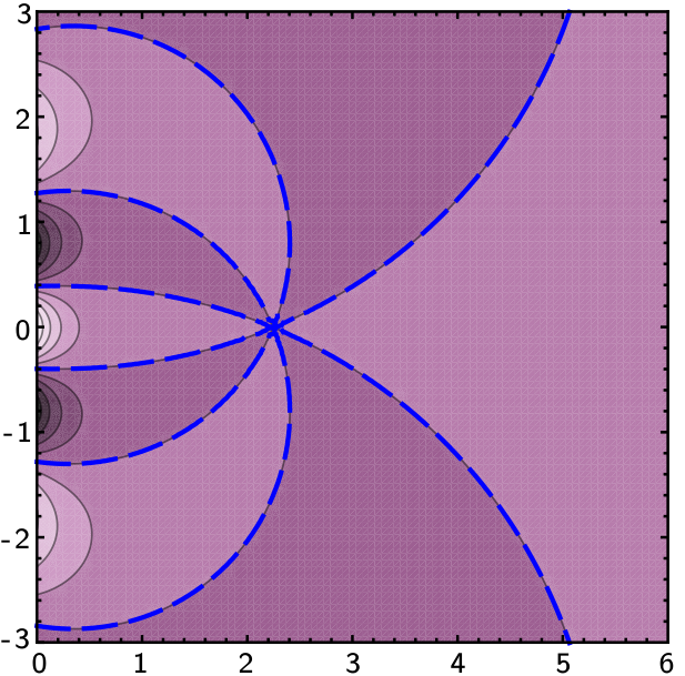
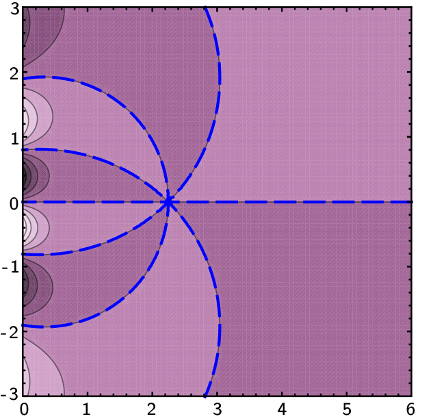
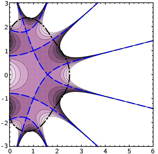
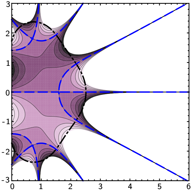

There are a few interesting things to note. First, FCF-relaxation expands the region of convergence in the complex plane dramatically for ESDIRK-33. However, there are other schemes (not shown here, for brevity) where FCF-relaxation provides little to no improvement. Also, note that the fine eigenvalue changes sign many times along the imaginary axis (in fact, the real part of changes signs times and the imaginary part ). Such behavior is very difficult to approximate with a coarse-grid time-stepping scheme, and provides another way to think about why imaginary eigenvalues and hyperbolic PDEs can be difficult for Parareal MGRIT. On a related note, using explicit time-stepping schemes in Parareal/MGRIT is inherently limited by ensuring a stable time step on the coarse grid, which makes naive application rare in numerical PDEs. However, when stability is satisfied on the coarse grid, Figure 3 (and similar plots for other explicit schemes) suggests that the domain of convergence pushes much closer against the imaginary axis for explicit schemes than implicit. Such observations may be useful in applying Parareal and MGRIT methods to systems of ODEs with imaginary eigenvalues, but less stringent stability requirements, wherein explicit integration may be a better choice than implicit.
3.2 Test case: The wave equation
The previous section considered the effects of imaginary eigenvalues on convergence of MGRiT and Parareal. Although true skew-symmetric operators are not particularly common, a similar character can be observed in other discretizations. In particular, writing the 2nd-order wave equation in first-order form and discretizing often leads to a spatial operator that is nearly skew-symmetric. Two-level and multilevel convergence theory for MGRIT based on eigenvalues was demonstrated to provide moderately accurate convergence estimates for small-scale discretizations of the second-order wave equation in MGRIT19. Here, we investigate the second-order wave equation further in the context of a finer spatiotemporal discretization, examining why eigenvalues provide reliable information on convergence, looking at the single-iteration bounds from Corollary 3, and discussing the broader implications.
The second-order wave equation in two spatial dimensions over domain is given by for with scalar solution and wave speed . This can be written equivalently as a system of PDEs that are first-order in time,
| (17) |
with initial and boundary conditions
3.2.1 Why eigenvalues:
Although the operator that arises from writing the second-order wave equation as first-order in time is not skew-adjoint, one can show that it (usually) has purely imaginary eigenvalues. Moreover, although not unitarily diagonalizable, the eigenvectors are only ill-conditioned in a specific, localized sense. As a result, the eigenvector convergence bounds provide an accurate measure of convergence.
Let be an eigenpair of the discretization of used in (17), for . For most standard discretizations, we have and the set forms an orthonormal basis of eigenvectors. Suppose this is the case. Expanding the block eigenvalue problem corresponding to (17),
yields a set of eigenpairs, grouped in conjugate pairs of the corresponding purely imaginary eigenvalues,
for . Although the -norm can be expressed in closed form, it is rather complicated. Instead, we claim that eigenvalue bounds (theoretically tight in the -norm) provide a good estimate of -convergence by considering the conditioning of eigenvectors.
Let denote a matrix with columns given by eigenvectors , ordered as above for . We can consider the conditioning of eigenvectors through the product
| (18) |
Notice that is a block-diagonal matrix with blocks corresponding to conjugate pairs of eigenvalues. The eigenvalues of the block are given by . Although (18) can be ill-conditioned for large , for spatial mesh size , the ill-conditioning is only between conjugate pairs of eigenvalues, and eigenvectors are otherwise orthogonal. Furthermore, the following Proposition proves that convergence bounds are symmetric across the real axis, that is, the convergence bound for eigenvector with spatial eigenvalue is equivalent to that for its conjugate . Together, these facts suggest the ill-conditioning between eigenvectors of conjugate pairs will not significantly affect the accuracy of bounds, and that tight eigenvalue convergence bounds for MGRIT in the -norm provide accurate estimates of performance in practice.
Proposition 1
Let and correspond to Runge-Kutta discretizations in time, as a function of a diagonalizable spatial operator , with eigenvalues . Then (tight) two-level convergence bounds of MGRIT derived in southworth19 as a function are symmetric across the real axis.
Proof
Recall from southworth19; 19c_mgrit, eigenvalues of and correspond to the Runge-Kutta stability functions applied to and , respectively, for coarsening factor . Also note that the stability function of a Runge-Kutta method can be written as a rational function of two polynomials with real coefficients, JCButcher_2016. As a result of the fundamental theorem of linear algebra . Thus for spatial eigenvalue , , , and , which implies that convergence bounds in Theorem 3.1 are symmetric across the real axis.
3.2.2 Observed convergence vs. bounds:
The first-order form (17) is implemented in MPI/C++ using second-order finite differences in space and various L-stable SDIRK time integration schemes (see (MGRIT19, Section SM3)). We consider 4096 points in the temporal domain and points in the spatial domain, with and , such that and , respectively. Two-level MGRIT with FCF-relaxation is tested for temporal coarsening factors XBraid, with a random initial space-time guess, an absolute convergence tolerance of , and a maximum of and iterations for SDIRK and ERK schemes, respectively. Figure 4 reports the geometric average (“Ave CF”) and worst-case (“Worst CF”) convergence factors for XBraid runs, along with estimates for the “Eval single it” bound from Corollary 3 by letting , the “Eval bound” as the eigenvalue form of the GSVD upper bound in Theorem 2.1, and the upper/lower bound from Theorem 3.1.
It turns out for this particular problem and discretization, convergence of Parareal/MGRIT requires an almost explicit restriction on time-step size. To that end, it is not likely to be competitive in practice vs. sequential time stepping. Nevertheless, our eigenvalue-based convergence theory provides a very accurate measure of convergence. In all cases, the theoretical lower and upper bound from Theorem 3.1 perfectly contain the worst observed convergence factor, with only a very small difference between the theoretical upper and lower bounds.
There are a number of other interesting things to note from Figure 4. First, both the general eigenvalue bound (“Eval bound”) and single iteration bound from Corollary 3 (”Eval single it”) are very pessimistic, sometimes many orders of magnitude larger than the worst observed convergence factor. As discussed previously and first demonstrated in 19c_mgrit, the size of the coarse problem, , is particularly relevant for problems with imaginary eigenvalues. Although the lower and upper bound converge to the “Eval bound” as , for small to moderate , reasonable convergence may be feasible in practice even if the limiting bound . Due to the relevance of , it is difficult to comment on the single iteration bound (because as derived, we let for an upper single-iteration bound). However, we note that the upper bound on all other iterations (“Upper bound”) appears to bound the worst-observed convergence factor, so the single-iteration bound on worst-case convergence appears not to be realized in practice, at least for this problem. It is also worth pointing out the difference between time-integration schemes in terms of convergence, with backward Euler being the most robust, followed by SDIRK3, and last SDIRK2. As discussed in 19c_mgrit for normal spatial operators, not all time-integration schemes are equal when it comes to convergence of Parareal and MGRIT, and robust convergence theory provides important information on choosing effective integration schemes.
Remark 1 (Superlinear convergence)
In Gander:2007jq, superlinear convergence of the Pareal algorithm is observed and discussed. We see similar behavior in Figure 4, where the worst observed convergence factor can be more than larger than the average convergence factor. In general, superlinear convergence would be expected as the exactness property of Parareal/MGRIT is approached. In addition, for non-normal operators, although the slowest converging mode may be observed in practice during some iteration, it does not necessarily stay in the error spectrum (and thus continue to yield slow(est) convergence) as iterations progress, due to the inherent rotation in powers of non-normal operators. The nonlinear setting introduces additional complications that may explain such behavior.
3.3 Test case: DG advection (diffusion)
Now we consider the time-dependent advection-diffusion equation,
| (19) |
on a 2D unit square domain discretized with linear discontinuous Galerkin elements. The discrete spatial operator, , for this problem is defined by , where is a mass matrix, and is the stiffness matrix associated with . The length of the time domain is always chosen to maintain the appropriate relationship between the spatial and temporal step sizes while also keeping 100 time points on the MGRIT coarse grid (for a variety of coarsening factors). Throughout, the initial condition is and the following time-dependent forcing function is used:
| (20) |
Backward Euler and a third-order, three-stage L-stable SDIRK scheme, denoted SDIRK3 are applied in time, and FCF-relaxation is used for all tests. Three different velocity fields are studied:
| (21) | |||
| (22) | |||
| (23) |
referred to as problems 1, 2, and 3 below. Note that problem 1 is a simple translation, problem 2 is a curved but non-recirculating flow, and problem 3 is a recirculating flow. The relative strength of the diffusion term is also varied in the results below, including a diffusion-dominated case, , an advection-dominated case, , and a pure advection case, . When backward Euler is used, the time step is set equal to the spatial step, , while for SDIRK3, , in order to obtain similar accuracy in both time and space.
Figure 5 shows various computed bounds compared with observed worst-case and average convergence factors (over 10 iterations) vs. MGRIT coarsening factor for each problem variation with different amounts of diffusion using backward Euler for time integration. The bounds shown are the “GSVD bound” from Theorem 2.1, the “Eval bound,” an equivalent eigenvalue form of this bound (see (southworth19, Theorem 13), and “Eval single it,” which is the bound from Corollary 3 as . The problem size is , where the spatial mesh has elements. This small problem size allows the bounds to be directly calculated: for the GSVD bound, it is possible to compute , and for the eigenvalue bounds, it is possible to compute the complete eigenvalue decomposition of the spatial operator, , and apply proper transformations to the eigenvalues to obtain eigenvalues of and .


In the diffusion-dominated case (left column of Figure 5), the GSVD and eigenvalue bounds agree well with each other (because the spatial operator is nearly symmetric), accurately predicting observed residual convergence factors for all problems. Similar to Section 3.2, the single iteration bound from Corollary 3 does not appear to be realized in practice.
In the advection-dominated and pure advection cases (middle and right columns of Figure 5), behavior of the bounds and observed convergence depends on the type of flow. In the non-recirculating examples, the GSVD bounds are more pessimistic compared to observed convergence, but still provide an upper bound on worst-case convergence, as expected. Conversely, the eigenvalue bounds on worst-case convergence become unreliable, sometimes undershooting the observed convergence factors by significant amounts. Recall that the eigenvalue bounds are tight in the -norm of the error, where is the matrix of eigenvectors. However, for the non-recirculating problems, the spatial operator is defective to machine precision, that is, the eigenvectors are nearly linearly dependent and is close to singular. Thus, tight bounds on convergence in the -norm are unlikely to provide an accurate measure of convergence in more standard norms, such as . In the recirculating case, is well conditioned. Then, similarly to the wave equation in Section 3.2, the eigenvalue bounds should provide a good approximation to the -norm, and, indeed, the GSVD and eigenvalue bounds agree well with each other accurately predict residual convergence factors.
Figure 6 shows the same set of results but using SDIRK3 for time integration instead of backward Euler and with a large time step to match accuracy in the temporal and spatial domains. Results here are qualitatively similar to those of backward Euler, although MGRIT convergence (both predicted and measured) is generally much swifter, especially for larger coarsening factors. Again, the GSVD and eigenvalue bounds accurately predict observed convergence in the diffusion-dominated case. In the advection-dominated and pure advection cases, again the eigenvalue bounds are not reliable for the non-recirculating flows, but all bounds otherwise accurately predict the observed convergence.


Figure 7 shows results for a somewhat larger problem, with spatial mesh of elements, to compare convergence estimates computed directly on a small problem size with observed convergence on more practical problem sizes. The length of the time domain is set according to the MGRIT coarsening factor such that there are always four levels in the MGRIT hierarchy (or again 100 time points on the coarse grid in the case of two-level) while preserving the previously stated time step to spatial step relationships. Although less tight than above, convergence estimates on the small problem size provide reasonable estimates of the larger problem in many cases, particularly for smaller coarsening factors. The difference in larger coarsening factors is likely because, e.g., for a mesh globally couples elements, while for a mesh remains a fairly sparse matrix. That is, the mode decomposition of for is likely a poor representation for .


Finally, we give insight in how the minimum over is realized in the TAP. Figure 8 and Figure 9 show the GSVD bounds (i.e. ) as a function of , for backward Euler and SDIRK3, respectively, and for each of the three problems and diffusion coefficients. A downside of the GSVD bounds in practice is the cost of computing for many values of . As shown, however, for the diffusion-dominated (nearly symmetric) problems, simply choosing is sufficient. Interestingly, SDIRK3 bounds have almost no dependence on for any problems, while backward Euler bounds tend to have a non-trivial dependence on (and demonstrate the symmetry in as discussed in Corollary 1). Nevertheless, accurate bounds for nonsymmetric problems do require sampling a moderate spacing of to achieve a realistic bound.


4 Conclusion
This paper furthers the theoretical understanding of convergence Parareal and MGRIT. A new, simpler derivation of measuring error and residual propagation operators is provided, which applies to linear time-dependent operators, and which may be a good starting point to develop improved convergence theory for the time-dependent setting. Theory from southworth19 on spatial operators that are independent of time is then reviewed, and several new results are proven, expanding the understanding of two-level convergence of linear MGRIT and Parareal. Discretizations of the two classical linear hyperbolic PDEs, linear advection (diffusion) and the second-order wave equation, are then analyzed and compared with the theory. Although neither naive implementation yields the rapid convergence desirable in practice, the theory is shown to accurately predict convergence on highly nonsymmetric and hyperbolic operators.
5 Appendix: Proofs
Proof (Proof of Theorem 2.2)
Here we consider a slightly modified coarsening of points: let the first points be F-points, followed by a C-point, followed by F-points, and so on, finishing with a C-point (as opposed to starting with a C-point). This is simply a theoretical tool that permits a cleaner analysis, but is not fundamental to the result. Then, define the so-called ideal restriction operator, via
Let be the orthogonal (column) block permutation matrix such that
where is the block row matrix . Then, from (4) and the fact that southworth19, the norm of residual and error propagation of MGRIT with F-relaxation is given by
where
Excuse the slight abuse of notation and denote ; that is, ignore the upper zero blocks in . Define a tentative pseudoinverse, , as
for some , and observe that
Three of the four properties of a pseudoinverse require that,
These three properties follow by picking such that , and , . Notice these are exactly the first three properties of a pseudoinverse of . To that end, define as the pseudoinverse of a full row rank operator,
Note that here, , and the fourth property of a pseudoinverse for , , follows immediately.
Recall the maximum singular value of is given by the minimum nonzero singular value of , which is equivalent to the minimum nonzero singular value of . Following from southworth19, the minimum nonzero eigenvalue of is bounded from above by the minimum eigenvalue of a block Toeplitz matrix, with real-valued matrix generating function
Let and denote the th eigenvalue and singular value of some operator, . Then,
Then,
and the result for follows.33 3 More detailed steps for this proof involving the block Toeplitz matrix and generating function can be found in similar derivations in southworth19; Serra:1998fm; Serra:1999ed; Miranda:2000is.
The case of follows an identical derivation with the modified operator , which follows from the right multiplication by in , which is effectively a right-diagonal scaling by . The cases of error propagation in the -norm follow a similar derivation based on .
Proof (Proof of Corollary 3)
The derivations follow a similar path as those in Theorem 2.2. However, when considering Toeplitz operators defined over the complex scalars (eigenvalues) as opposed to operators, additional results hold. In particular, the previous lower bound (that is, necessary condition) is now a tight bound in norm, which follows from a closed form for the eigenvalues of a perturbation to the first or last entry in a tridiagonal Toeplitz matrix Losonczi1992; DafonsecaKowalenko2019. Scalar values also lead to a tighter asymptotic bound, as opposed to , which is derived from the existence of a second-order zero of , when the Toeplitz generating function is defined over complex scalars as opposed to operators Serra:1998fm. Analogous derivations for each of these steps can be found in the diagonalizable case in southworth19, and the steps follow easily when coupled with the pseduoinverse derived in Theorem 2.2.
Acknowledgments
Los Alamos National Laboratory report number LA-UR-20-28395. This work was supported by Lawrence Livermore National Laboratory under contract B634212, and under the Nicholas C. Metropolis Fellowshop from the Laboratory Directed Research and Development program of Los Alamos National Laboratory.
References
- [1] Guillaume Bal. On the Convergence and the Stability of the Parareal Algorithm to Solve Partial Differential Equations. In Domain Decomposition Methods in Science and Engineering, pages 425–432. Springer, Berlin, Berlin/Heidelberg, 2005.
- [2] J. C. Butcher. Numerical methods for ordinary differential equations. John Wiley & Sons, Ltd., Chichester, third edition, 2016. With a foreword by J. M. Sanz-Serna.
- [3] CM Da Fonseca and V Kowalenko. Eigenpairs of a family of tridiagonal matrices: three decades later. Acta Mathematica Hungarica, pages 1–14.
- [4] V A Dobrev, Tz V Kolev, N A Petersson, and J B Schroder. Two-level Convergence Theory for Multigrid Reduction in Time (MGRIT). SIAM Journal on Scientific Computing, 39(5):S501–S527, 2017.
- [5] R D Falgout, S Friedhoff, Tz V Kolev, S P MacLachlan, and J B Schroder. Parallel Time Integration with Multigrid. SIAM Journal on Scientific Computing, 36(6):C635–C661, 2014.
- [6] S Friedhoff and B S Southworth. On “optimal” h-independent convergence of Parareal and multigrid-reduction-in-time using Runge-Kutta time integration. Numerical Linear Algebra with Applications, page e2301, 2020.
- [7] M J Gander and Ernst Hairer. Nonlinear Convergence Analysis for the Parareal Algorithm. In Domain decomposition methods in science and engineering XVII, pages 45–56. Springer, Berlin, Berlin, Heidelberg, 2008.
- [8] M J Gander and S Vandewalle. On the Superlinear and Linear Convergence of the Parareal Algorithm. In Domain Decomposition Methods in Science and Engineering XVI, pages 291–298. Springer, Berlin, Berlin, Heidelberg, 2007.
- [9] A Hessenthaler, B S Southworth, D Nordsletten, O Röhrle, R D Falgout, and J B Schroder. Multilevel convergence analysis of multigrid-reduction-in-time. SIAM Journal on Scientific Computing, 42(2):A771–A796, 2020.
- [10] J-L Lions, Y Maday, and G Turinici. Resolution d’EDP par un Schema en Temps ”Parareel”. C. R. Acad. Sci. Paris Ser. I Math., 332(661-668), 2001.
- [11] L Losonczi. Eigenvalues and eigenvectors of some tridiagonal matrices. Acta Mathematica Hungarica, 60(3-4):309–322, 1992.
- [12] T A Manteuffel, K J Ressel, and G Starke. A boundary functional for the least-squares finite-element solution of neutron transport problems. SIAM Journal on Numerical Analysis, 37(2):556–586, 1999.
- [13] M Miranda and P Tilli. Asymptotic Spectra of Hermitian Block Toeplitz Matrices and Preconditioning Results. SIAM Journal on Matrix Analysis and Applications, 21(3):867–881, January 2000.
- [14] Daniel Ruprecht. Convergence of Parareal with Spatial Coarsening. PAMM, 14(1):1031–1034, December 2014.
- [15] S Serra. On the Extreme Eigenvalues of Hermitian (Block) Toeplitz Matrices. Linear Algebra and its Applications, 270(1-3):109–129, February 1998.
- [16] S Serra. Spectral and Computational Analysis of Block Toeplitz Matrices Having Nonnegative Definite Matrix-Valued Generating Functions. BIT, 39(1):152–175, March 1999.
- [17] B S Southworth. Necessary Conditions and Tight Two-level Convergence Bounds for Parareal and Multigrid Reduction in Time. SIAM J. Matrix Anal. Appl., 40(2):564–608, 2019.
- [18] S-L Wu and T Zhou. Convergence Analysis for Three Parareal Solvers. SIAM Journal on Scientific Computing, 37(2):A970–A992, January 2015.
- [19] Shu-Lin Wu. Convergence analysis of some second-order parareal algorithms. IMA Journal of Numerical Analysis, 35(3):1315–1341, 2015.
- [20] XBraid: Parallel multigrid in time. http://llnl.gov/casc/xbraid.
- [21] I N Zwaan and M E Hochstenbach. Generalized davidson and multidirectional-type methods for the generalized singular value decomposition. arXiv preprint arXiv:1705.06120, 2017.