Measure Transport with Kernel Stein Discrepancy
Abstract
Measure transport underpins several recent algorithms for posterior approximation in the Bayesian context, wherein a transport map is sought to minimise the Kullback–Leibler divergence (KLD) from the posterior to the approximation. The KLD is a strong mode of convergence, requiring absolute continuity of measures and placing restrictions on which transport maps can be permitted. Here we propose to minimise a kernel Stein discrepancy (KSD) instead, requiring only that the set of transport maps is dense in an sense and demonstrating how this condition can be validated. The consistency of the associated posterior approximation is established and empirical results suggest that KSD is competitive and more flexible alternative to KLD for measure transport.
1 Introduction
A popular and constructive approach to approximation of complicated distributions is to learn a transformation from a simpler reference distribution. Within machine learning, neural networks are often used to provide flexible families of transformations which can be optimised by stochastic gradient descent on a suitable objective, with variational autoencoders (Kingma and Welling 2013; Rezende et al. 2014), generative adversarial networks (Goodfellow et al. 2014), generative moment matching networks (Li et al. 2015; Dziugaite et al. 2015) and normalizing flows (Rezende and Mohamed 2015; Kingma et al. 2016; Dinh et al. 2016; Papamakarios et al. 2019; Kobyzev et al. 2020) all fitting in this framework. The principal application for such generative models is distribution estimation; samples are provided from the target distribution and the task is to fit a distribution to these samples. Parallel developments within applied mathematics view the transformation as a transport map performing measure transport (Marzouk et al. 2016; Parno and Marzouk 2018). The principal application for measure transport is posterior approximation; an un-normalised density function defines the complicated distribution and the task is to approximate it. In this paper we study posterior approximation, noting that the flexible transformations developed in the machine learning literature can also be applied to this task.
Measure transport provides a powerful computational tool for Bayesian inference in settings that can be challenging for standard approaches, such as Markov chain Monte Carlo (MCMC) or mean field variational inference. For example, even sophisticated MCMC methods can fail when a posterior is concentrated around a sub-manifold of the parameter space (Livingstone and Zanella 2019; Au et al. 2020), while it can be relatively straight-forward to define a transport map whose image is the sub-manifold (Parno and Marzouk 2018; Brehmer and Cranmer 2020). Likewise, mean field variational inference methods can perform poorly in this context, since independence assumptions can be strongly violated (Blei et al. 2017).
Let be a measurable space equipped with a probability measure , representing the posterior to be approximated. The task that we consider in this paper is to elicit a second measurable space , equipped with a probability measure , and a measurable function , such that the push-forward (i.e. the measure produced by applying to samples from ) approximates , in a sense to be specified. It is further desired that should be a “simple” distribution that is easily sampled. In contrast to the literature on normalising flows, it is not stipulated that should be a bijection, since we wish to allow for situations where and have different cardinalities or where is supported on a sub-manifold.
A natural starting point is a notion of discrepancy between two probability measures, and , on , with the property that if and only if and are equal. Then one selects a measurable space and associated probability measure and seeks a solution to
| (1) |
over a suitable set of measurable functions from to . A popular choice of is the Kullback-Leibler divergence (KLD), giving rise to variational inference (Blei et al. 2017), but other discrepancies can be considered (Ranganath et al. 2016). The problem in (1) can be augmented to include also the selection of and , if desired.
The solution of (1) provides an approximation to whose quality will depend on the set and the discrepancy . This motivates us to consider the choice of and , taking into account considerations that go beyond computational tractability. For example, a desirable property would be that, for a sequence of probability measures , if then in some suitable sense. For , the KLD11 1 We use the notation ., it holds that implies converges to in total variation, from Pinsker’s inequality (Tsybakov 2009). This is a strong mode of convergence, requiring absolute continuity of measures that may be difficult to ensure when the posterior is concentrated near to a sub-manifold. Accordingly, the use of KLD for measure transport places strong and potentially impractical restrictions on which maps are permitted (e.g. Marzouk et al. 2016; Parno and Marzouk 2018, required that is a diffeomorphism with on ). This motivates us in this paper to consider the use of an alternative discrepancy , corresponding to a weaker mode of convergence, for posterior approximation using measure transport. The advantage of discrepancy measures inducing weaker modes of convergence has also motivated recent developments in generative adversarial networks (Arjovsky et al. 2017).
Our contributions are as follows:
- •
We propose kernel Stein discrepancy (KSD) as an alternative to KLD for posterior approximation using measure transport, showing that KSD renders (1) tractable for standard stochastic optimisation methods (Proposition 1).
- •
Using properties of KSD we are able to establish consistency under explicit and verifiable assumptions on , and (Theorem 2).
- •
Our theoretical assumptions are weak – we do not even require to be a bijection – and are verified for a particular class of neural network (Proposition 3). In particular, we do not require and to be defined on the same space, allowing quite flexible mappings to be constructed.
- •
Empirical results support KSD as a competitive alternative to KLD for measure transport.
Earlier work on this topic appears limited to Hu et al. 2018, who trained a neural network with KSD. Here we consider general transport maps and we establish consistency of the method, which these earlier authors did not. We note also that gradient flows provide an alternative (implicit) approach to measure transport (Liu and Wang 2016).
Outline:
2 Methods
This section introduces measure transport using KSD. In Section 2.1 and Section 2.2 we recall mathematical definitions from measure transport and Hilbert spaces, respectively; in Section 2.3 we recall the definition and properties of KSD; in Section 2.4 we formally define our proposed method, and in Section 2.5 we present some parametric families that can be employed.
Notation:
The set of probability measures on a measurable space is denoted and a point mass at is denoted . For let . For and , let denote weak convergence of the sequence of measures to . The Euclidean norm on is denoted . Partial derivatives are denoted . For a function the gradient is defined as . For a function , the divergence is defined as .
Our main results in this paper concern the Euclidean space , but in some parts of the paper, such as Section 2.1, it is possible to state definitions at a greater level of generality at no additional effort - in such situations we do so.
2.1 Measure Transport
A Borel space is a topological space equipped with its Borel -algebra, denoted . Throughout this paper we restrict attention to Borel spaces and . Let and . In the parlance of measure transport, is the reference and the target. Let be a measurable function and define the pushforward of through as the probability measure that assigns mass to each . Here denotes the pre-image of under . Such a function is called a transport map from to if .
Faced with a complicated distribution , if one can express using a transport map and a distribution that can be sampled, then samples from can be generated by applying to samples from . This idea underpins elementary methods for numerical simulation of random variables (Devroye 2013). However, in posterior approximation it will not typically be straightforward to identify a transport map and at best one can seek an approximate transport map, for which approximates in some sense to be specified. In this paper we seek approximations in the sense of KSD, which is formally introduced in Section 2.3 and requires concepts in Section 2.2, next.
2.2 Hilbert Spaces
A Hilbert space is a complete inner product space; in this paper we use subscripts, such as , to denote the associated inner product. Given two Hilbert spaces , , the Cartesian product is again a Hilbert space equipped with the inner product . In what follows we let denote the unit ball in a Hilbert space .
From the Moore–Aronszajn theorem (Aronszajn 1950), any symmetric positive definite function defines a unique reproducing kernel Hilbert space of real-valued functions on , denoted and with inner-product denoted . Indeed, is a Hilbert space characterised by the properties (i) for all , (ii) for all , . Reproducing kernels are central to KSD, as described next.
2.3 Kernel Stein Discrepancy
Stein discrepancies were introduced in Gorham and Mackey 2015 to provide a notion of discrepancy that is computable in the Bayesian statistical context. In this paper we focus on so-called kernel Stein discrepancy (Liu et al. 2016; Chwialkowski et al. 2016; Gorham and Mackey 2017, KSD;) since this has lower computational overhead compared to the original proposal of Gorham and Mackey 2015.
The construction of KSD relies on Stein’s method (Stein 1972) where, for a possibly complicated probability measure of interest, one identifies a Stein set and a Stein operator , such that acts on elements to return functions with the property that
| (2) |
for all . A Stein discrepancy uses the extent to which (2) is violated to quantify the discrepancy between and :
Note that is not symmetric in its arguments. For and suitably regular , which admits a positive and differentiable density function , Liu et al. 2016; Chwialkowski et al. 2016 showed that one may take to be a set of smooth vector fields and to be a carefully chosen differential operator on . More precisely, and letting , we have Theorem 1 below, which is due to Gorham and Mackey 2017:
Definition 1 (Eberle 2015).
A probability measure is called distantly dissipative if , where
Theorem 1.
Suppose that is distantly dissipative. For some , and , let
| (3) | |||
| (4) |
Then (2) holds. Moreover, if , then .
The kernel appearing in (3) is called the inverse multi-quadric kernel. It is known that the elements of are smooth functions, which justifies the application of the differential operator. The last part of Theorem 1 clarifies why KSD is useful; convergence in KSD controls the standard notion of weak convergence of measures to .
KSD, in contrast to KLD, is well-defined when the approximating measure and the target differ in their support. Moreover, in some situations KSD can be exactly computed: from Liu et al. 2016 or equivalently Chwialkowski et al. 2016,
| (5) | ||||
| (6) |
It follows that KSD can be exactly computed whenever has a finite support and can be evaluated on this support:
| (7) |
Computation of (7) can proceed with available up to an unknown normalisation constant, facilitating application in the Bayesian context. Now we are in a position to present our proposed method.
2.4 Measure Transport with KSD
Our proposed method for posterior approximation is simply stated at a high level; we attempt to solve (1) with and over a set of candidate functions indexed by a finite-dimensional parameter . That is, we aim to solve
| (8) |
Discussion of the choice of is deferred until Section 2.5. Compared to previous approaches to measure transport using KLD (Rezende and Mohamed 2015; Kingma et al. 2016; Marzouk et al. 2016; Parno and Marzouk 2018), KSD is arguably more computationally and theoretically tractable; the computational aspects will now be described.
The solution of (8) is equivalent to minimisation of the function over . In order to employ state-of-the-art algorithms for stochastic optimisation, an unbiased estimator for the gradient is required. A naive starting point would be to differentiate the expression for the KSD of an empirical measure in (7), however the resulting V-statistic is biased. Under weak conditions, we establish instead the following unbiased estimator (a U-statistic) for the gradient:
Proposition 1.
Let be an open set. Assume that
- (A1)
is measurable;
- (A2)
;
- (A3)
;
and that ,
- (A4)
is continuous.
Then
where the expectation is taken with respect to independent samples .
All proofs are contained in Appendix A. The assumptions on amount to assumptions on , and , by virtue of (6). It is not difficult to find explicit assumptions on , and that imply (A1-4), but these may be stronger than required and we prefer to present the most general result.
Armed with an unbiased estimator of the gradient, we can employ a stochastic optimisation approach, such as stochastic gradient descent (Robbins and Monro 1951, SGD;) or adaptive moment estimation (Kingma and Ba 2015, Adam;). See Kushner and Yin 2003; Ruder 2016. For the results reported in the main text we used Adam, with initialised as described in Section C.1, but other choices were investigated (see Section C.2).
2.5 Parametric Transport Maps
In this section we describe some existing classes of transport map that are compatible with KSD measure transport. From Proposition 1 we see that measure transport using KSD does not impose strong assumptions on the transport map. Indeed, compared to KLD (Rezende and Mohamed 2015; Kingma et al. 2016; Marzouk et al. 2016; Parno and Marzouk 2018) we do not require that is a diffeomorphism ( need not even be continuous, nor a bijection), making our framework considerably more general. This additional flexibility may allow measure to be transported more efficiently, using simpler maps. That being said, if one wishes to compute the density of (in addition to sampling from ), then a diffeomorphism, along with the usual change-of-variables formula, should be used.
Triangular Maps:
Rosenblatt 1952 and Knothe et al. 1957 observed that, for admitting densities, a transport map can without loss of generality be sought in the triangular form
| (9) |
where each and (Bogachev et al. 2005, Lemma 2.1). The triangular form was used in Marzouk et al. 2016; Parno and Marzouk 2018, since the Jacobian determinant, that is required when using KLD (but not KSD), can exploit the fact that is triangular to maintain linear complexity in .
Maps from Measure Transport:
In the context of a triangular map , Marzouk et al. 2016 and Parno and Marzouk 2018 considered several parametric models for the components , including polynomials, radial basis functions and monotone parameterisations of the form
for functions and . The monotone parameterisation ensures that on , which facilitates computation of the density of , as required for KLD22 2 For polynomials and radial basis functions, these authors only enforced locally, introducing an additional approximation error in evaluation of KLD; such issues do not arise with KSD..
Maps from Normalising Flows:
The principal application of normalising flows is density estimation (Papamakarios et al. 2019; Kobyzev et al. 2020), but the parametric families of transport map used in this literature can also be used for posterior approximation (Rezende and Mohamed 2015). A normalising flow is required to be a diffeomorphism with the property that the density of can be computed. A popular choice that exploits the triangular form (9) is an autoregressive flow , where is a monotonic transformation of parameterised by , e.g. an affine transformation where outputs and . For instance, Kingma et al. 2016 proposed inverse autoregressive flows (IAF), taking . Here is elementwise multiplication and and are vectors output by an autoregressive neural network: one designed so that depend on only through for . In Huang et al. 2018, was the output of a monotonic neural network and the resulting flow was called a neural autoregressive flow (NAF). Compositions of normalising flows can also be considered, of the form
| (10) |
where each is itself a normalising flow e.g. a IAF. For instance, Dinh et al. 2014 proposed using coupling layers of the form , where and is a bijection. These only update the first components of , so they are typically composed with permutations.
Regardless of the provenance of a transport map , all free parameters of are collectively denoted , and are to be estimated. The suitability of a parametric set of candidate maps in combination with KSD is studied both empirically in Section 4 and theoretically, next.
3 Theoretical Assessment
In Section 3.1 we affirm basic conditions on and for a transport map to exist. In Section 3.2 we establish sufficient conditions for the consistency of our method and in Section 3.3 we consider a particular class of transport maps based on neural networks, to demonstrate how our conditions on the transport map can be explicitly validated.
3.1 Existence of an Transport Map
For a complete separable metric space , recall that the Wasserstein space of order is defined by taking some and
where the definition is in fact independent of the choice of (Villani 2009, Definition 6.4). For existence of a transport map, we make the following assumptions on and :
Assumption 1 (Assumptions on ).
The reference measure , where is a complete separable metric space, and for all .
Assumption 2 (Assumptions on ).
The target measure has a strictly positive density on .
These assumptions guarantee the existence of a transport map with regularity, as shown in the following result:
Of course, such a transport map will not be unique in general.
3.2 Consistent Posterior Approximation
The setting for our theoretical analysis considers a sequence of parametric classes of transport map, where intuitively provides a more flexible class of map as is increased. For example, could represent the class of triangular maps comprising of th order polynomials, or a class of normalising flows comprising of layers in (10).
Assumption 3 (Assumptions on ).
There exists a subset containing an element for which . The sequence satisfies with for and is a dense set in .
Proposition 2 provides sufficient conditions for the set in 3 to exist; the additional content of 3 ensures that is rich enough to consistently approximate an exact transport map, in principle at least. Next, we state our consistency result:
Theorem 2.
The statement in (11) accommodates the reality that, although finding the global optimum will typically be impractical, one can realistically expect to find an element that achieves an almost-as-low value of KSD, e.g. using a stochastic optimisation method. To our knowledge, no comparable consistency guarantees exist for measure transport using KLD.
3.3 Validating our Assumptions on
Recall that earlier work on measure transport placed strong restrictions on the set of maps , requiring each map to be a diffeomorphism with non-vanishing Jacobian determinant. In contrast, our assumptions on are almost trivial; we do not require smoothness and there is not a bijection requirement. Our assumptions can be satisfied in principle whenever is a complete separable metric space, since then is separable (Cohn 2013, Proposition 3.4.5) and admits a Schauder basis , so we may take for 3 to hold. In practice we are able to verify 3 for quite non-trivial classes of map . To demonstrate, one such example is presented next:
We consider deep neural networks with multi-layer perceptron architecture and ReLU activation functions Let denote the set of such ReLU neural networks with layers and width at most . See Definition 4 in Section A.4 for a formal definition.
Proposition 3.
The maps in Proposition 3 are not bijections, illustrating the greater flexibility of KSD compared to KLD for measure transport. This completes our theoretical discussion, and our attention now turns to empirical assessment.
4 Empirical Assessment
The purpose of this section is to investigate whether KSD is competitive with KLD for measure transport. Section 4.1 compares both approaches using a variety of transport maps and a synthetic test-bed. Then, in Sections 4.2 and 4.3 we consider more realistic posterior approximation problems arising from, respectively, a biochemical oxygen model and a parametric differential equation model.
In all experiments we used the kernel (3) with , , (other choices were investigated in Section C.5), the stochastic optimiser Adam with batch size and learning rate (other choices were investigated in Section C.2), and the reference distribution was taken to be a standard Gaussian on (other choices were considered in Section C.4). Code to reproduce these results is available at https://github.com/MatthewAlexanderFisher/MTKSD.
4.1 Synthetic Test-Bed

First we consider a set of synthetic examples that have previously been used to motivate measure transport as an alternative to MCMC. Three targets were considered; is a sinusoidal density, is a banana density and is multimodal; these are formally defined in Section B.2. Results for and are displayed in Figure 1. The convergence of the approximation to the target is shown for KSD and the corresponding approximation after iterations of Adam is shown for KLD. Since, for both objectives, one iteration requires evaluations of or its gradient, this represents a total of calls to or its gradient. The corresponding approximation produced using an adaptive Hamiltonian Monte Carlo (HMC) algorithm (Hoffman and Gelman 2014; Betancourt 2017) is shown, where the HMC chains were terminated once evaluations of or its gradient had been performed. Both and present challenges for HMC that, to some extent, can be overcome using measure transport.
The results in Figure 1 are for a fixed class of transport map, but now we report a systematic comparison of KSD and KLD. The majority of maps that we consider are diffeomorphic (in order that KLD can be used), implemented in Pyro (Bingham et al. 2018). Since KSD does not place such requirements on the transport map, we also report results for a (non-bijective) ReLU neural network. Our performance measure is an estimate of the Wasserstein-1 distance between the target and approximate distributions computed using samples (see Section B.1 for details). Results are detailed in Table 1. Overall, there is no clear sense in which KSD out-performs KLD or vice versa; KSD performed best on , KLD performed best on , and for the results were mixed. We conclude that these objectives offer similar performance for measure transport. However, KLD cannot be applied to the ReLU neural network (denoted N/A in Table 1) due to the strong constraints on the mapping that are required by KLD.
| Sinusoidal | Banana | Multimodal | |||||
|---|---|---|---|---|---|---|---|
| Transport Map | KSD | KLD | KSD | KLD | KSD | KLD | |
| IAF | 0.38 | 0.20 | 0.07 | 0.67 | 1.1 | ||
| IAF (stable) | 0.35 | 0.16 | 0.11 | 0.61 | 0.62 | ||
| NAF | 0.55 | 0.39 | 0.025 | 0.095 | 0.11 | ||
| SAF | 0.23 | 0.20 | 0.18 | 0.30 | 0.48 | ||
| B-NAF | 0.78 | 0.70 | 0.18 | 1.0 | 0.99 | ||
| Polynomial (cubic) | 0.40 | 0.25 | 0.059 | 0.51 | 0.43 | ||
| IAF mixture | 0.61 | 0.19 | 0.14 | 0.037 | 0.036 | ||
| ReLU network | 0.71 | N/A | 0.43 | N/A | 0.22 | N/A | |
Two discussion points are now highlighted: First, it is known that certain normalising flows can capture multiple modes due to their flexibility, however others cannot (Huang et al. 2018). One solution is to consider a mixture of transport maps; i.e. with reference distribution and mixing weights satisfying . This idea has been explored recently in Pires and Figueiredo 2020. In Table 1 we report results using mixtures of inverse autoregressive flows (IAF). As one might hope, these approximations were successful in finding each of the modes in , but fared relatively worse for and . Second, since in Adam we are using a Monte Carlo estimator of the gradient, it is natural to ask whether a quasi Monte Carlo estimator would offer an improvement (Wenzel et al. 2018). This was investigated and our results are reported in Section C.3.
4.2 Biochemical Oxygen Demand Model
Next we reproduce an experiment that was used to illustrate measure transport using KLD in Parno and Marzouk 2018. The task is parameter inference in a dimensional oxygen demand model, of the form , where is the biochemical oxygen demand at time , a measure of the consumption of oxygen in a given water column sample due to the decay of organic matter (Sullivan et al. 2010). The parameters to be inferred are . Full details of the prior and the likelihood are contained in Section B.3.
For our experiment, we trained a block neural autoregressive flow33 3 This class of transport map was experimentally observed to outperform the other classes we considered. using iterations of Adam. Results are presented in Figure 2. Unlike the synthetic experiments, we no longer have a closed form for the target ; however, this problem was amenable to MCMC and a long run of HMC ( iterations, thinned by a factor of 100) provided a gold standard, allowing us to approximate the Wasserstein-1 distance from to as in Section 4.1. For the KSD-based method, we obtained a Wasserstein-1 distance of , while KLD achieved . Although the Wasserstein-1 distance for KSD is larger than that for KLD, both values are close to the noise floor for our approximation of the Wasserstein-1 distance; two independent runs of HMC ( iterations, thinned by a factor of 100), differed in Wasserstein-1 distance by 0.022. We therefore conclude that KSD and KLD performed comparably on this task.

4.3 Generalised Lotka-Volterra Model
Our final experiment is a realistic inference problems involving a non-trivial likelihood. Following Parno and Marzouk 2018, we consider parameter inference for a generalised Lotka–Volterra model
| (12) | ||||
where are the predator and prey populations respectively at time and and , along with the initial conditions and , are parameters to be inferred. Together, these parameters were inferred from a noisy dataset, with the prior and likelihood reported in Section B.4. This task is realistic and yet amenable to MCMC; the latter is an essential requirement to allow us to provide a gold standard against which to assess KSD and KLD, and we again used an extended run of HMC.
For this experiment, the B-NAF class and iterations of Adam were used. The gradients, required both for HMC and KSD measure transport, were computed using automatic differentiation through the numerical integrator used to solve (12), implemented in the torchdiffeq Python package (Chen et al. 2018).
For the KSD-based method, we obtained an approximate Wasserstein-1 distance from to of , while KLD achieved . The noise floor for our approximation of the Wasserstein-1 distance in this case was . We therefore conclude that KSD and KLD also performed comparably on this more challenging task.
5 Discussion
This paper proposed and studied measure transport using KSD, which can be seen as an instance of operator variational inference (Ranganath et al. 2016). Our findings suggest that KSD is a suitable variational objective for measure transport; we observed empirical performance comparable with that of KLD, yet only minimal and verifiable conditions on the map were required.
There are three potential limitations of KSD compared to KLD: First, the parameters of the kernel must be specified, and a poor choice of kernel parameters can result in poor approximation; see Section C.5. It would be interesting to explore whether adversarial maximisation of KSD with respect to the kernel parameters, while minimising KSD over the choice of transport map, offers a solution (Grathwohl et al. 2020). Second, while only first order derivatives are required for KLD, gradient-based optimisation of KSD requires second order derivatives of . In most automatic differentiation frameworks, and for most models, this is possible at little extra computational cost, but sometimes this will present difficulties e.g. for models with differential equations involved. Third, it is known that score-based variational objectives can sometimes exhibit pathologies (Wenliang 2020); some of these are illustrated in Section C.8.
Several recent works explored the possibility of combining measure transport with Monte Carlo (Salimans et al. 2015; Wolf et al. 2016; Hoffman 2017; Caterini et al. 2018; Prangle 2019; Thin et al. 2020) and it would also be interesting to consider the use of KSD in that context. Related, for both KSD and KLD there is freedom to select the space and the reference distribution . This could also be handled within the optimisation framework, but further work would be needed to determine how these additional degrees of freedom should be parametrised.
Acknowledgements: MAF was supported by the EPSRC Centre for Doctoral Training in Cloud Computing for Big Data EP/L015358/1 at Newcastle University, UK. THN was supported by a Fulbright scholarship, an American Australian Association scholarship and a Roberta Sykes scholarship. MMG and CJO were supported by the Lloyd’s Register Foundation programme on data-centric engineering at the Alan Turing Institute, UK. The authors thank Onur Teymur for helpful comments on the manuscript.
References
- Aliprantis and Burkinshaw [1998] Charalambos D Aliprantis and Owen Burkinshaw. Principles of Real Analysis. Academic Press, 1998.
- Arjovsky et al. [2017] Martin Arjovsky, Soumith Chintala, and Léon Bottou. Wasserstein generative adversarial networks. In Proceedings of the 34th International Conference on Machine Learning-Volume 70, pages 214–223, 2017.
- Aronszajn [1950] Nachman Aronszajn. Theory of reproducing kernels. Transactions of the American Mathematical Society, 68(3):337–404, 1950.
- Arora et al. [2018] Raman Arora, Amitabh Basu, Poorya Mianjy, and Anirbit Mukherjee. Understanding deep neural networks with rectified linear units. In Proceedings of the 6th International Conference on Learning Representations, 2018.
- Au et al. [2020] Khai Xiang Au, Matthew M Graham, and Alexandre H Thiery. Manifold lifting: Scaling MCMC to the vanishing noise regime. arXiv:2003.03950, 2020.
- Betancourt [2017] Michael Betancourt. A conceptual introduction to Hamiltonian Monte Carlo. arXiv:1701.02434, 2017.
- Betancourt et al. [2014] MJ Betancourt, Simon Byrne, and Mark Girolami. Optimizing the integrator step size for Hamiltonian Monte Carlo. arXiv:1411.6669, 2014.
- Billingsley [1979] Patrick Billingsley. Probability and Measure. John Wiley and Sons, 1979.
- Bingham et al. [2018] Eli Bingham, Jonathan P. Chen, Martin Jankowiak, Fritz Obermeyer, Neeraj Pradhan, Theofanis Karaletsos, Rohit Singh, Paul Szerlip, Paul Horsfall, and Noah D. Goodman. Pyro: Deep universal probabilistic programming. Journal of Machine Learning Research, 20(18):403, 2018.
- Blei et al. [2017] David M. Blei, Alp Kucukelbir, and Jon D. McAuliffe. Variational inference: A review for statisticians. Journal of the American Statistical Association, 112(518):859–877, 2017.
- Bogachev et al. [2005] V I Bogachev, A V Kolesnikov, and K V Medvedev. Triangular transformations of measures. Sbornik: Mathematics, 196(3):309–335, apr 2005. doi: 10.1070/sm2005v196n03abeh000882. URL https://doi.org/10.1070%2Fsm2005v196n03abeh000882.
- Border [2016] KC Border. Differentiating an integral: Leibniz’ rule. Technical report, Caltech Division of the Humanities and Social Sciences, 2016.
- Brehmer and Cranmer [2020] Johann Brehmer and Kyle Cranmer. Flows for simultaneous manifold learning and density estimation. arXiv:2003.13913, 2020.
- Buchholz et al. [2018] Alexander Buchholz, Florian Wenzel, and Stephan Mandt. Quasi-Monte Carlo variational inference, 2018.
- Cao et al. [2019] Nicola De Cao, Ivan Titov, and Wilker Aziz. Block neural autoregressive flow. In Proceedings of the 35th Conference on Uncertainty in Artificial Intelligence, 2019.
- Carpenter et al. [2017] Bob Carpenter, Andrew Gelman, Matthew D Hoffman, Daniel Lee, Ben Goodrich, Michael Betancourt, Marcus Brubaker, Jiqiang Guo, Peter Li, and Allen Riddell. Stan: A probabilistic programming language. Journal of Statistical Software, 76(1), 2017.
- Caterini et al. [2018] Anthony L Caterini, Arnaud Doucet, and Dino Sejdinovic. Hamiltonian variational auto-encoder. In Proceedings of the 32nd Conference on Neural Information Processing Systems, pages 8167–8177, 2018.
- Chen et al. [2018] Ricky T. Q. Chen, Yulia Rubanova, Jesse Bettencourt, and David Duvenaud. Neural ordinary differential equations. In Proceedings of the 32nd Conference on Neural Information Processing Systems, 2018.
- Chwialkowski et al. [2016] Kacper Chwialkowski, Heiko Strathmann, and Arthur Gretton. A kernel test of goodness of fit. In Proceedings of the 33rd International Conference on Machine Learning, 2016.
- Cohn [2013] Donald L Cohn. Measure Theory. Springer, 2013.
- Devroye [2013] Luc Devroye. Non-Uniform Random Variable Generation. Springer, 2013.
- Dinh et al. [2014] Laurent Dinh, David Krueger, and Yoshua Bengio. NICE: Non-linear independent components estimation. arXiv:1410.8516, 2014.
- Dinh et al. [2016] Laurent Dinh, Jascha Sohl-Dickstein, and Samy Bengio. Density estimation using real NVP. arXiv:1605.08803, 2016.
- Dolatabadi et al. [2020] Hadi M. Dolatabadi, Sarah Erfani, and Christopher Leckie. Invertible generative modeling using linear rational splines. arXiv:2001.05168, 2020.
- Durkan et al. [2019] Conor Durkan, Artur Bekasov, Iain Murray, and George Papamakarios. Neural spline flows. In Proceedings of the 33rd Conference on Neural Information Processing Systems, 2019.
- Dziugaite et al. [2015] Gintare Karolina Dziugaite, Daniel M Roy, and Zoubin Ghahramani. Training generative neural networks via maximum mean discrepancy optimization. In Proceedings of the 31st Conference on Uncertainty in Artificial Intelligence, pages 258–267, 2015.
- Eberle [2015] Andreas Eberle. Reflection couplings and contraction rates for diffusions. Probability Theory and Related Fields, 166(3-4):851–886, Oct 2015. ISSN 1432-2064.
- Flamary and Courty [2017] Rémi Flamary and Nicolas Courty. POT: Python Optimal Transport library. https://pythonot.github.io/, 2017.
- Garreau et al. [2018] Damien Garreau, Wittawat Jitkrittum, and Motonobu Kanagawa. Large sample analysis of the median heuristic, 2018.
- Germain et al. [2015] Mathieu Germain, Karol Gregor, Iain Murray, and Hugo Larochelle. MADE: Masked autoencoder for distribution estimation. In Proceedings of the 32nd International Conference on Machine Learning, 2015.
- Glynn [1986] Peter W Glynn. Stochastic approximation for Monte Carlo optimization. In Proceedings of the 18th Winter Simulation Conference, pages 356–365, 1986.
- Goodfellow et al. [2014] Ian Goodfellow, Jean Pouget-Abadie, Mehdi Mirza, Bing Xu, David Warde-Farley, Sherjil Ozair, Aaron Courville, and Yoshua Bengio. Generative adversarial nets. In Proceedings of the 28th Conference on Neural Information Processing Systems, pages 2672–2680, 2014.
- Gorham and Mackey [2015] Jackson Gorham and Lester Mackey. Measuring sample quality with Stein’s method. In Proceedings of the 29th Conference on Neural Information Processing Systems, 2015.
- Gorham and Mackey [2017] Jackson Gorham and Lester Mackey. Measuring sample quality with kernels. In Proceedings of the 34th International Conference on Machine Learning, 2017.
- Graham [2020] Matthew M Graham. Mici: Python implementations of manifold MCMC methods. https://github.com/matt-graham/mici, November 2020.
- Grathwohl et al. [2020] Will Grathwohl, Kuan-Chieh Wang, Jörn-Henrik Jacobsen, David Duvenaud, and Richard Zemel. Learning the Stein discrepancy for training and evaluating energy-based models without sampling. In Proceedings of the 37th International Conference on Machine Learning, 2020.
- Hoffman [2017] Matthew D Hoffman. Learning deep latent Gaussian models with Markov chain Monte Carlo. In Proceedings of the 34th International Conference on Machine Learning, pages 1510–1519, 2017.
- Hoffman and Gelman [2014] Matthew D Hoffman and Andrew Gelman. The No-U-Turn sampler: Adaptively setting path lengths in Hamiltonian Monte Carlo. Journal of Machine Learning Research, 15(1):1593–1623, 2014.
- Hu et al. [2018] Tianyang Hu, Zixiang Chen, Hanxi Sun, Jincheng Bai, Mao Ye, and Guang Cheng. Stein neural sampler. arXiv:1810.03545, 2018.
- Huang et al. [2018] Chin-Wei Huang, David Krueger, Alexandre Lacoste, and Aaron Courville. Neural autoregressive flows. In Proceedings of the 35th International Conference on Machine Learning, 2018.
- Izmailov et al. [2020] Pavel Izmailov, Polina Kirichenko, Marc Finzi, and Andrew Gordon Wilson. Semi-supervised learning with normalizing flows. In Proceedings of the 37th International Conference on Machine Learning, 2020.
- Kechris [1995] Alexander Kechris. Classical Descriptive Set Theory. Springer, 1995.
- Kingma and Welling [2013] D. P. Kingma and M. Welling. Auto-encoding variational Bayes. In Proceedings of the 2nd International Conference on Learning Representations, 2013.
- Kingma and Ba [2015] Diederik P. Kingma and Jimmy Ba. Adam: A method for stochastic optimization. In Proceedings of the 3rd International Conference on Learning Representations, 2015.
- Kingma et al. [2016] Durk P Kingma, Tim Salimans, Rafal Jozefowicz, Xi Chen, Ilya Sutskever, and Max Welling. Improved variational inference with inverse autoregressive flow. In Proceedings of the 30th Conference on Neural Information Processing Systems, 2016.
- Knothe et al. [1957] Herbert Knothe et al. Contributions to the theory of convex bodies. The Michigan Mathematical Journal, 4(1):39–52, 1957.
- Kobyzev et al. [2020] Ivan Kobyzev, Simon Prince, and Marcus Brubaker. Normalizing flows: An introduction and review of current methods. IEEE Transactions on Pattern Analysis and Machine Intelligence, 2020. ISSN 1939-3539. URL http://dx.doi.org/10.1109/TPAMI.2020.2992934. To appear.
- Kushner and Yin [2003] Harold Kushner and G. George Yin. Stochastic Approximation and Recursive Algorithms and Applications. Springer Science & Business Media, 2003.
- L’Ecuyer [1995] Pierre L’Ecuyer. Note: On the interchange of derivative and expectation for likelihood ratio derivative estimators. Management Science, 41:738–747, 04 1995. doi: 10.1287/mnsc.41.4.738.
- Li et al. [2015] Yujia Li, Kevin Swersky, and Rich Zemel. Generative moment matching networks. In Proceedings of the 32nd International Conference on Machine Learning, pages 1718–1727, 2015.
- Liu and Wang [2016] Qiang Liu and Dilin Wang. Stein variational gradient descent: A general purpose Bayesian inference algorithm. In Proceedings of the 30th Conference on Neural Information Processing Systems, 2016.
- Liu et al. [2016] Qiang Liu, Jason D. Lee, and Michael I. Jordan. A kernelized Stein discrepancy for goodness-of-fit tests and model evaluation. In Proceedings of the 33rd International Conference on Machine Learning, 2016.
- Livingstone and Zanella [2019] Samuel Livingstone and Giacomo Zanella. On the robustness of gradient-based MCMC algorithms. arXiv:1908.11812, 2019.
- Marzouk et al. [2016] Youssef Marzouk, Tarek Moselhy, Matthew Parno, and Alessio Spantini. Sampling via Measure Transport: An Introduction. Handbook of Uncertainty Quantification, page 1–41, 2016.
- Papamakarios et al. [2019] George Papamakarios, Eric Nalisnick, Danilo Jimenez Rezende, Shakir Mohamed, and Balaji Lakshminarayanan. Normalizing flows for probabilistic modeling and inference. arXiv:1912.02762, 2019.
- Parno and Marzouk [2018] Matthew D Parno and Youssef M Marzouk. Transport map accelerated Markov chain Monte Carlo. SIAM/ASA Journal on Uncertainty Quantification, 6(2):645–682, 2018.
- Pires and Figueiredo [2020] Guilherme G. P. Freitas Pires and Mário A. T. Figueiredo. Variational mixture of normalizing flows. arXiv:2009.00585, 2020.
- Prangle [2019] Dennis Prangle. Distilling importance sampling. arXiv:1910.03632, 2019.
- Ranganath et al. [2016] Rajesh Ranganath, Dustin Tran, Jaan Altosaar, and David Blei. Operator variational inference. In Proceedings of the 30th Annual Conference on Neural Information Processing Systems, pages 496–504, 2016.
- Rezende and Mohamed [2015] Danilo Jimenez Rezende and Shakir Mohamed. Variational inference with normalizing flows. 2015.
- Rezende et al. [2014] Danilo Jimenez Rezende, Shakir Mohamed, and Daan Wierstra. Stochastic backpropagation and variational inference in deep latent Gaussian models. In Proceedings of the 31st International Conference on Machine Learning, 2014.
- Robbins and Monro [1951] Herbert Robbins and Sutton Monro. A stochastic approximation method. The Annals of Mathematical Statistics, 22(3):400–407, 09 1951. URL https://doi.org/10.1214/aoms/1177729586.
- Rockwood [2015] Larry L. Rockwood. Introduction to Population Ecology. Wiley-Blackwell, 2015. ISBN 978-1-118-94757-9.
- Rosenblatt [1952] Murray Rosenblatt. Remarks on a multivariate transformation. The Annals of Mathematical Statistics, 23(3):470–472, 1952.
- Ruder [2016] Sebastian Ruder. An overview of gradient descent optimization algorithms. arXiv:1609.04747, 2016.
- Salimans et al. [2015] Tim Salimans, Diederik Kingma, and Max Welling. Markov chain Monte Carlo and variational inference: Bridging the gap. In Proceedings of the 32nd International Conference on Machine Learning, pages 1218–1226, 2015.
- Stein [1972] Charles Stein. A bound for the error in the normal approximation to the distribution of a sum of dependent random variables. In Proceedings of the Sixth Berkeley Symposium on Mathematical Statistics and Probability, Volume 2: Probability Theory, pages 583–602, Berkeley, Calif., 1972. University of California Press. URL https://projecteuclid.org/euclid.bsmsp/1200514239.
- Sullivan et al. [2010] Annett B. Sullivan, Dean M. Snyder, and Stewart A. Rounds. Controls on biochemical oxygen demand in the upper Klamath river, Oregon. Chemical Geology, 269(1):12 – 21, 2010. ISSN 0009-2541. doi: https://doi.org/10.1016/j.chemgeo.2009.08.007. URL http://www.sciencedirect.com/science/article/pii/S0009254109003404.
- Thin et al. [2020] Achille Thin, Nikita Kotelevskii, Jean-Stanislas Denain, Leo Grinsztajn, Alain Durmus, Maxim Panov, and Eric Moulines. MetFlow: A new efficient method for bridging the gap between Markov chain Monte Carlo and variational inference. arXiv:2002.12253, 2020.
- Tsybakov [2009] Alexandre B. Tsybakov. Introduction to Nonparametric Estimation. Springer Series in Statistics. Springer, 2009. ISBN 978-0-387-79052-7.
- Villani [2009] Cedric Villani. Optimal Transport, Old and New. Springer, 2009.
- Wenliang [2020] Li K Wenliang. Blindness of score-based methods to isolated components and mixing proportions. arXiv:2008.10087, 2020.
- Wenzel et al. [2018] Florian Wenzel, Alexander Buchholz, and Stephan Mandt. Quasi-Monte Carlo flows. In Proceedings of the 3rd Workshop on Bayesian Deep Learning, 2018.
- Wolf et al. [2016] Christopher Wolf, Maximilian Karl, and Patrick van der Smagt. Variational inference with Hamiltonian Monte Carlo. arXiv:1609.08203, 2016.
Supplement
This supplement is structured as follows:
- •
Appendix A contains the proofs of the theory developed in the main text: Proposition 1 (Section A.1), Proposition 2 (Section A.2), Theorem 2 (Section A.3) and Proposition 3 (Section A.4).
- •
Appendix B contains the computational details and extensions to the experiments detailed in Section 4. Section B.1 explains how the Wasserstein-1 distance was computed as our performance metric. Section B.2 provides the full details of the synthetic test-bed experiments used in Section 4.1. Similarly, Section B.3 and Section B.4 provides the full details of the biochemical oxygen demand experiment of Section 4.2 and Section 4.3 respectively.
- •
Appendix C contains further investigations into the methods presented in the main paper. Section C.1 discusses the sensitivity to initialisation and explains how the transport maps were initialised for the experiments of Section 4. Section C.2 explores variations on the stochastic optimisation method. Section C.3 explores the use of quasi Monte Carlo in the stochastic approximation of gradients for KSD. In Section C.4, we investigate the effect of the changing the reference distribution. In Section C.5, we explore the effect of the length-scale parameter on KSD-based measure transport. Section C.6 explores the effect of the input dimension in the ReLU network transport map. In Section C.7, we investigate KSD-based measure transport using a (biased) V-statistic estimator of KSD against the unbiased U-statistic estimator that was used for the experiments presented in the main text. Finally, in Section C.8, we document certain pathological behaviours experienced when using KSD for measure transport and offer potential remedies.
Appendix A Proof of Theoretical Results
This section contains the proofs for all novel theoretical results stated in the main text. In Section A.1 we present the proof of Proposition 1; in Section A.2 we present the proof of Proposition 2; the proof of Theorem 2 is contained in Section A.3, and finally, the proof of Proposition 3 is in Section A.4.
A.1 Proof of Proposition 1
The argument involved in the proof of Proposition 1 requires differentiation under an integral. The measure-theoretic calculus result that we exploit to justify the interchange of differentiation and integration (Lemma 2 below) requires the following mathematical concepts:
Definition 2.
Let be a measurable space and let be a topological space. A function is a Carathéodory function if for each the map is measurable and for each the map is continuous.
Definition 3.
Let be a measurable space equipped with a measure and let be a topological space. A function is locally uniformly integrably bounded if for every there is a non-negative measurable function such that , and there exists a neighbourhood of such that for all we have .
The following sufficient condition for a function to be locally uniformly integrably bounded will be used:
Lemma 1.
In the setting of Definition 3, let be an open set and assume further that, for each , the function is continuous and that, for each , the integral exists. Then is locally uniformly integrably bounded.
Proof.
Fix and . Since is continuous in and is open, we can find a neighbourhood of on which for all . Take , recalling that the absolute value of a measurable function is measurable and sums of measurable functions are measurable. Then and , as required. ∎
Lemma 2 (Differentiate under the integral).
Let be a measurable space equipped with a measure , let be an open set and let be a Carathéodory function. Assume further that is locally uniformly integrably bounded and that, for each and each , the function is locally uniformly integrably bounded. Then the function defined by
is continuously differentiable and
Proof.
This standard result can be found, for example, in Aliprantis and Burkinshaw 1998, Billingsley 1979, with the statement here based on the account in Border 2016. ∎
The proof of Proposition 1 can now be presented:
Proof of Proposition 1.
Using (5) and the reparametrisation trick [Glynn 1986, L’Ecuyer 1995, Kingma and Welling 2013]:
| (13) |
From Lemma 2, the preconditions of Proposition 1 justify the interchange of the derivative and the expectation in (13). Indeed, in the setting of Lemma 2 we identify , and where . That is a Carathéodory function follows from (A1) and (A4) of Proposition 1, where we note that (A4) implies is continuous. That is locally uniformly integrably bounded follows from assumptions (A2) and (A4) together with Lemma 1. Similarly, that is locally uniformly integrably bounded follows from assumptions (A3) and (A4) together with Lemma 1. Thus the preconditions of Lemma 2 hold.
Interchanging the derivative with the expectation gives that
as claimed. ∎
Note that we presented stronger conditions in Proposition 1 than are required. This was to control the length of the main text, but it is immediately clear from the proof of Proposition 1 that these conditions can be weakened to those that are required for Lemma 2 to hold.
A.2 Proof of Proposition 2
First we present an existence result in Proposition 4, before considering regularity of the associated transport map. Recall that in this paper all measurable spaces and are equipped with their respective Borel -algebras and . A separable complete metric space equipped with its Borel -algebra is called a standard Borel space. A measure is said to be continuous if for all . A map is called a Borel isomorphism if is a bijection and both and are Borel measurable. A fundamental result that we will exploit is known as the isomorphism theorem for measures:
Theorem 3 (Isomorphism Theorem).
Let be a standard Borel space and be continuous. Then there is a Borel isomorphism with , where is the Lebesgue measure restricted to .
Proof.
This result can be found as Theorem 17.41 in Kechris 1995. ∎
Proposition 4.
Suppose that and are separable complete metric spaces and suppose that and are such that and for all and . Then there exists a measurable function such that .
Proof.
Our assumptions imply that , are standard Borel spaces and , are continuous. Thus from Theorem 3, there exists a Borel isomorphism such that and a Borel isomorphism such that . Then is measurable and satisfies , as required. ∎
Now we can present the proof of Proposition 2.
Proof of Proposition 2.
1 ensures that is a separable complete metric space and for all . 2 restricts attention to , meaning that is a separable complete metric space, and requires to admit a density on , meaning that for all . Thus the existence of a transport map from to is guaranteed by Proposition 4.
It remains to show that, for any such transport map, . To this end, we have that
where a change of variables was used at and the final inequality follows from the assumption that in 2. ∎
A.3 Proof of Theorem 2
Recall that for the (first) Wasserstein distance is defined as [Villani 2009, Remark 6.5]
| (14) |
where and is the Lipschitz seminorm on . Our proof of Theorem 2 is based on the following result that relates convergence in to convergence in KSD:
Proposition 5 (Wasserstein Controls KSD).
Let be symmetric positive definite with , and continuous and bounded for all . Let admit a density function such that is Lipschitz with . Let denote the KSD based on and , as defined in (7). Then a sequence satisfies whenever .
Proof.
This result is Proposition 9 of Gorham and Mackey 2017. ∎
Recall that in this paper is always assumed to be a Borel space. The following result is also required:
Lemma 3 ( Controls Wasserstein).
Let and let . Then we have the bound .
Proof.
From the definition of the (first) Wasserstein distance, we have
If then for all , and so
where the second inequality is Jensen’s inequality. ∎
Our final ingredient is a basic result on the inverse multi-quadric kernel:
Lemma 4 (Derivatives of the Inverse Multi-quadric Kernel).
Proof.
For let . Recall that a polynomial is said to have maximal degree , where is the largest integer for which for some . Let
Then and is closed under the action of each of the differential operators , . Indeed, we have from the product rule that
and
| (15) |
where has been implicitly defined. Since , it follows that the terms , and appearing in (15) are polynomials in of maximal degree . Thus, from (15), is a polynomial of maximal degree , showing that the set is closed under the action of .
Since the differential operator is obtained by repeated application of operators of the form , and since it is clear that all elements of are bounded on , the claim is established. ∎
Now we can prove Theorem 2:
Proof of Theorem 2.
First note that our preconditions are a superset of those required for Theorem 1. Thus the conclusion of Theorem 1 holds; namely, if then . From (11) we have that and agree in the limit. Thus it is sufficient to show that in the limit.
Second, note that our preconditions are also a superset of those required for Proposition 5. Indeed, from Lemma 4 the inverse multi-quadric kernel in (3) is infinitely differentiable with derivatives of all orders bounded. Thus it is sufficient to show that in the limit.
From 1 and 2 and Proposition 2, there exists a map with . From 3, there is a set such that and the set is dense in . Thus there exists a sequence with in .
For each , let denote the smallest integer for which , which is well-defined since . Let , so that is a non-decreasing sequence with in the limit. Note that, since for all , we have .
Thus from Lemma 3 we conclude that
| (16) |
in the limit. Again, since for , the sequence is non-increasing and, from (16), it has a subsequence that converges to 0. It follows that , as required.
∎
A.4 Proof of Proposition 3
Recall the rectified linear unit activation function , which we consider to be applied componentwise when .
Definition 4 (Deep ReLU Neural Network).
A deep ReLU neural network with hidden layers from to is a function of the form
where , , is an affine transformation, is a linear transformation, is the input dimension, is the output dimension, and , , is the width of the th hidden layer. The set of all deep ReLU neural networks with hidden layers from to with maximum width is denoted and we let .
The following, essentially trivial observation will be useful:
Proposition 6.
.
Proof.
For fixed , there is a canonical injection from into that concatenates the neural networks width-wise, to form a single neural network with width . Since every element of belongs to for a sufficiently large , the claim is established. ∎
Here we introduce the shorthand for where is the Lebesgue measure on . The following result on the approximation properties of deep ReLU neural networks, which derives from the fact that the set of continuous piecewise linear functions is dense in , will be required.
Proposition 7.
For every function and every , there exists a function such that , where .
Proof.
For , this result is a special case of Theorem 2.3 in Arora et al. 2018, which derives from the fact that continuous piecewise linear functions are dense in .
For general , we observe that for each component we can find a function with . Then, letting , we have that and
Finally, we note from Proposition 6 that . ∎
Now we present the proof of Proposition 3:
Proof of Proposition 3.
From 1 and 2 and Proposition 2 there exists such that . Let , so that is satisfied.
From the statement of Proposition 3 we have with . From Definition 4 it is therefore clear that whenever and that .
Thus all parts of 3 have been verified except the part that requires to be dense in ; i.e. that the set is dense in the Hilbert space . To establish this last part, we will make use of Proposition 7:
Let and . From the definition of , there exists such that, for each of the coordinates ,
Let
Our assumption that admits a positive and continuous density on ensures that , since
| (17) |
where the supremum in (17) is finite, since is well-defined and continuous on the compact set . Let also , which is well-defined since we assumed to be continuous and bounded on . Then, since , we may evoke Proposition 7 to find a function such that . It remains to check that approximates in . To this end, we can use the triangle inequality in and the fact that to see that
Since was arbitrary, this argument shows that the set is dense in , as required. ∎
Appendix B Computational Details
This section provides full details for the experiments presented in Section 4.
B.1 Performance Metric
To estimate the Wasserstein-1 distance between the target distribution and approximations we computed the earth mover distance (EMD) between two uniformly weighted empirical measures, each formed from samples from their respective distributions and with the Euclidean distance between the samples used to construct the cost matrix. The EMD was computed using an implementation in the Python Optimal Transport (POT) package [Flamary and Courty 2017]. For the target distribution, independent samples were used in the synthetic test bed in Section 4.1 and thinned samples from a long HMC chain were used for the real examples in Sections 4.2 and 4.3. For the approximate distribution, independent samples from were used.
B.2 Details of the Synthetic Test Bed
To assess the proposed methods, we considered the following bivariate densities
where is the univariate Gaussian density with mean and variance , and is the bivariate Gaussian density with mean vector and covariance matrix . The parameter choices for the sinusoidal experiment were and . The parameter choices for the banana experiment were and . The parameter choices for the multi-modal experiment were and . The target densities can be seen in Figure 3.

Computational costs for each method in terms of number of target evaluations and CPU wall-clock time against performance are shown, respectively, in Figure 4 and Figure 5. From Figure 4, there is no clear sense in which KSD or KLD out-performs the other across the different synthetic tests; this is in line with the conclusion of Section 4.1. For CPU wall-clock time in Figure 5, KSD-based measure transport is approximately three to five times slower than its KLD counterpart. However, note that our implementation of KSD is not production code and further performance gains can certainly be achieved.
We now discuss the implementations details of all the methods used in Section 4.1. In all our measure transport implementations, unless specified otherwise, we used existing implementations in Pyro [Bingham et al. 2018]. Furthermore, the reference measure used for synthetic tests was the standard Gaussian on .
Hamiltonian Monte Carlo:
We used an adaptive HMC algorithm in which the integrator step size was automatically adjusted using a dual-averaging algorithm in a warm-up phase to give an average acceptance statistic of 0.8 [Betancourt et al. 2014] and the number of integrator steps per transition was set dynamically by expanding the trajectory until a termination criterion was met [Hoffman and Gelman 2014, Betancourt 2017]. We used the HMC implementations in the Python package [Graham 2020], with the dual-averaging adaptation algorithm settings following the defaults used in Stan [Carpenter et al. 2017]. Only the post-warm-up samples were included in estimates of the discrepancies and density plots.
In the following, the autoregressive neural networks that we specify are the Masked Autoencoders for Density Estimation (MADE) of Germain et al. 2015; the only difference being, that there is no sigmoidal non-linearity applied to the output layer.
Inverse Autoregressive Flow (IAF):
Recall from Section 2.5, that an autoregressive flow is of the form , where and . The IAF flow of Kingma et al. 2016 takes to be the th output of an autoregressive neural network and to be an affine transform of the form
where and are outputs from . Note that the coefficient of is forced to be positive, this ensures the resulting transport map is monotonic.
For each synthetic test problem, we used a single IAF where the dimensionality of the hidden units in the single hidden layer of the underlying autoregressive neural network was . The underlying autoregressive neural network used the ReLU activation function. The IAF was initialised using the same default random initialisation in both the KSD and KLD experiments. iterations of Adam were used, with learning rate .
Stable Inverse Autoregressive Flow (IAF stable):
Closely related to an IAF, a stable IAF was introduced in Kingma et al. 2016 in order to improve numerical stability. The only difference being that the is of the form
where and are outputs from and
where, for , we consider sigmoid to be applied component-wise. Since sigmoid is monotonic, the resulting transport map is again monotonic. The restriction may limit the expressibility of the transport map compared to standard IAF, but this at the expense of increased numerical stability.
For each synthetic test problem, we used a single stable IAF where the dimensionality of the hidden units in the single hidden layer of the underlying autoregressive neural network was . The underlying autoregressive neural network used the ReLU activation function. The stable IAF was initialised using the same default random initialisation in both the KSD and KLD experiments. iterations of Adam were used, with learning rate .
Neural Autoregressive Flow (NAF):
A NAF, introduced in Huang et al. 2018, is again an autoregressive flow which, compared to the preceding IAF and stable IAF, offers greater flexibility and a universality guarantee. The autoregressive conditioner is again taken as an autoregressive neural network and takes the form of a monotonic neural network whose weights and biases are the output of the conditioner . Monotonicity of is guaranteed by using strictly positive weights and strictly monotonic activation functions.
The particular implementation of that we used in Pyro uses what is termed a deep sigmoidal flow (DSF) in Huang et al. 2018. A DSF is a single layer dense neural network with a sigmoidal activation function. Furthermore, in order to increase the effective range of , an inverse sigmoid function is taken on the output layer. However, this inverse sigmoid function has domain and thus the weights and biases of the output layer must be constrained such that this composition can be well defined. In a DSF, this is achieved by having no bias term on the output layer and constraining the output layer’s weights, , to satisfy . Thus the output term of a DSF is a convex combination of the output of the hidden layer. The overall transformation of a DSF is thus of the form
where is an affine transformation and is a convex combination. iterations of Adam were used, with learning rate .
Following Huang et al. 2018, for each synthetic test problem, we used a single DSF style NAF, where the dimensionality of the hidden sigmoid units in each DSF was and the dimensionality of the hidden units in the single hidden layer of the underlying autoregressive neural network was . The underlying autoregressive neural network used the ReLU activation function. Note that the dimensionality of th output of this autoregressive neural network is , due to the weight terms and the bias terms in each DSF. The NAF was initialised using the same default random initialisation in both the KSD and KLD experiments.
Spline Autoregressive Flow (SAF):
A SAF, developed in Durkan et al. 2019 and Dolatabadi et al. 2020, is again an autoregressive flow that takes as a piecewise monotonic rational polynomial function (a spline) on an interval and the identity otherwise. A rational polynomial function is the ratio of two polynomials. In Durkan et al. 2019, the polynomial was taken as quadratic polynomial and in Dolatabadi et al. 2020, the polynomial was taken as a linear polynomial. The parameters controlling each rational polynomial function, are the output of an autoregressive neural network. We also note that originally the spline transform was implemented in the context of coupling flows, rather than autoregressive flows.
For each synthetic test problem, we used a single SAF based on rational linear splines with pieces defined on the interval . The underlying autoregressive neural network had two hidden layers, each of dimension . The SAF was initialised using the same default random initialisation in both the KSD and KLD experiments. iterations of Adam were used, with learning rate .
Block Neural Autoregressive Flow (B-NAF):
A B-NAF, introduced in Cao et al. 2019, is similar in spirit to the NAF. It is an autoregressive flow, where is a neural network. The difference is now that the weights and biases of are not the output of an autoregressive conditioner network ; instead, the parameters of the neural network are learned directly. In a B-NAF, the affine transformations , for , used at a given layer are always in a lower triangular block form
where , each and is the freely parameterised bias term . The positivity-ensuring transform enforces monotonicity. Bijectivity is further ensured by using bijective activation functions. Note that this particular form of affine transformation place restrictions on the structure of the neural network. For instance, the hidden dimensions must be a multiple of the input dimension . Similarly to NAFs, B-NAFs also have a universality result.
For each synthetic test problem we used a single B-NAF with the activation function and . The B-NAF used had two hidden layers and was of the form
with lower triangular block affine transformations , and . The B-NAF was initialised using the same default random initialisation in both the KSD and KLD experiments. iterations of Adam were used, with learning rate .
Polynomial (Cubic):
Polynomials were first put forward as possible parametric transport maps in measure transport [Marzouk et al. 2016, Parno and Marzouk 2018]. In Marzouk et al. 2016, each component of a polynomial transport map , was parameterised as a linear basis expansion of multivariate polynomials . Each is further parameterised with respect to a vector of polynomial degrees as a product of univariate polynomials of the form
where each is a univariate degree polynomial. These can come from orthogonal families of polynomials or simply be monomials. For instance, we could take the to be orthogonal with respect to the reference measure of the transport map. The th component of can thus be written as
where each . This is a flexible parameterisation that can enforce triangularity through the choices of the . For example, a natural choice to enforce triangularity would be to take to consist of vectors such that . The first constraint enforces triangularity and the second restraint ensures that the total degree of the resulting polynomials would be no greater than a given . In higher dimensions, this may not be practical since the number of parameters grows quickly as the dimension increases. Thus other constraints on were put forward, such as removing mixed terms in the basis.
An issue with this approach is that the resulting maps are not monotonic for all values of the coefficients . In Marzouk et al. 2016 and Parno and Marzouk 2018, monotonicity was constrained locally at a given set of samples from the reference distribution. Due to the triangular nature of the transport map, this effectively results in a finite set of linear constraints of the form for and . In our implementation of KLD-based polynomial transport for the synthetic test bed, we found that this approach was not necessary since, in each case, the resulting Jacobian always had a positive determinant.
In our synthetic experiments, we used the the natural choice of the that enforces triangularity that we previously discussed with and took the as simple monomials. The overall transport map was thus a multivariate cubic polynomial of the form
The polynomial transport map was initialised to the identity in all synthetic experiments. iterations of Adam were used, with learning rate .
IAF mixture:
A mixture of transport maps is a distribution of the form
where the are each a transport map of a given form, the are possibly distinct reference distributions and the mixing weights satisfy . This is a very flexible extension to using just a single transport map. Furthermore, in principle, both the number of mixing components and the mixing weights could be learnt. For example, the weights could be the output of a neural network with softmax applied to the output layer44 4 The th component of the softmax function is of the form ., as was done in Pires and Figueiredo 2020.
For simplicity, in our synthetic experiments, we a priori set and further set each . We took each as a single IAF, where the dimensionality of the hidden units in the single hidden layer was . Refer to our discussion of an IAF in Section B.2 or Kingma et al. 2016 for full details of an IAF. The were initialised as Gaussians with means respectively and each with identity covariance matrix. iterations of Adam were used, with learning rate .
ReLU network:
Refer to Definition 4 for the definition of a deep ReLU network.
For our synthetic experiments, we implemented a deep ReLU network for each synthetic test problem. When using KSD, the transport map need not be a diffeomorpism and so, to illustrate this flexibility, the input dimension of the ReLU network for each experiment was taken as (while the dimension of the target was 2). For each problem, the ReLU network had two hidden layers and was of the form
where , and are affine transformations and is the ReLU non-linearity, defined in Section A.4. Using the default random initialisation of these ReLU networks nearly always resulted in bad output. So, for each synthetic experiment, the ReLU network was pretrained for iterations of KSD-based measure transport using Adam with learning rate , in order to approximate the reference distribution . That is, we pretrained the ReLU network in order to initialise it close to . After pretraining, further iterations of Adam were used for each synthetic test problem, with learning rate .
B.3 Details of the Biochemical Oxygen Model Experiment
Derivation of the Posterior:
Following on from Section 4.2, recall that the two-dimensional biochemical oxygen demand model is of the form
Due to the positivity constraints on and , we perform inference on the log of the parameters and thus consider the model
Synthetic data were generated at times with the parameter values and , with observations corrupted by independent mean Gaussian errors with variance . See Figure 6 for a plot of with these given parameter values alongside our generated synthetic data.
The likelihood is thus of the form
The prior specified for was . The resulting posterior density is thus of the form
Methodology:
Our choice of parametric transport map was a Block Neural Autoregressive Flow (B-NAF) of Cao et al. 2019. We used the same B-NAF as the one used in Section 4.1, where we again used a B-NAF with two hidden layers of the form
with lower triangular block affine transformations , and . Refer to Section B.2 or to Cao et al. 2019 for a full description of a B-NAF. The lengthscale used for KSD was . We again used the Adam optimiser, with default learning rate with iterations for each method.
Results:
See Figure 2 for samples obtained from each resulting transport map. The KSD-based method obtained a Wasserstein-1 distance of and the KLD-based method obtained a Wasserstein-1 distance of . Refer to Section B.1 for details on how this was calculated. Figure 7 plots using samples from the prior and the approximate posterior using KSD-based measure transport.
B.4 Details of the Generalised Lotka–Volterra Model Experiment
Prior Specification:
Recall that, from Section 4.3, the generalised Lotka–Volterra model we considered was of the form
with parameters . These parameters are physical quantities, see Rockwood 2015 for their full meaning. Due to the positivity constraints on these parameter values, similar to our biochemical oxygen demand experiment Section 4.2, we again perform inference on the log of the parameters. We thus consider the model
where we perform inference on the parameter .
After an investigation of the sensitivities of the solutions of the ODE with respect to the parameter values, we specified the following independent prior
Letting be the vector of these given mean values and the diagonal matrix with these given variances on the diagonal, we have . This specification results in log-normal priors on the exponentiated parameters.
Synthetic data were generated at times with parameter values ; these data were perturbed by independent mean Gaussian errors with variance . See Figure 8 for a plot of the solution of the generalised Lotka-Volterra model with these given parameters alongside our generated synthetic data.
The likelihood is thus of the form
where are the solutions of generalised Lotka-Volterra ODE (12) with given parameter . The resulting posterior density is thus of the form
Methodology:
We used the torchdiffeq Python library [Chen et al. 2018] in order to numerically solve the Lotka–Volterra model and further utilised Pytorch’s automatic differentiation capabilities to propagate gradients through the solver. In our implementation, we used the default Dormand-Prince Runge-Kutta method. The reference measure used was the prior. Our choice of parametric transport map was a B-NAF with , of the form
with lower triangular block affine transformations , and . Refer to Section B.2 or to Cao et al. 2019 for a full description of a B-NAF.
For both the KSD and KLD experiments, we used the same random initialisation of the B-NAF and pretrained on iterations of KLD-based measure transport on the prior (the reference measure), to ensure that the initial pushforward of samples through the B-NAF resulted in non-degenerate solutions of the Lotka–Volterra model.
The lengthscale used for KSD was and we again used the Adam optimiser, with default learning rate with iterations for each method.
Results:
The KSD-based method obtained a Wasserstein-1 distance of , whereas the KLD-based method acheived a Wasserstein-1 distance of . Refer to Section B.1 for details on how this was calculated. The resulting approximating distributions for both the KSD and KLD methods are plotted in Figure 9.


Appendix C Further Investigations
Here we report a series of further investigations, that explore specific aspects of KSD-based measure transport in more detail.
C.1 Initialisation of Parameters in the Transport Map
Both KLD and KSD-based measure transport can be sensitive to the initialisation of the parameters in a given transport map. This is, for instance, evidenced in Figure 15. In our experiments we generally used a random initialisation as specified by their implementations in Pyro [Bingham et al. 2018]. In Appendix B, we specify for each experiment in the main paper what initialisation was used and whether we pretrained on the reference distribution .
A general remedy for poor initialisation is either to pretrain on the reference distribution. This was done in our applied examples in Section 4.2 and Section 4.3. Alternatively, in a Bayesian inference context one could pretrain on the prior distribution instead. The latter approach may be advantageous since we are guaranteed that the target’s support is contained within the prior’s support.
C.2 Investigating the Choice of Stochastic Optimisation Method
In all our experiments in Section 4, we used the Adam optimiser of Kingma and Ba 2015 with a fixed batch size of and with a varying number of iterations. In this section we explore how the output of KSD-based measure transport, with a fixed number of iterations of stochastic optimisation, interacts with the batch size as well as the stochastic optimisation method used. We fixed the target distribution as the multimodal problem and considered only B-NAF as our transport map with standard Gaussian reference distribution. Results are shown in Table 2, where we report the Wasserstein-1 distance using samples (see Section B.1 for more details). We pretrained the B-NAF on the reference distribution using KLD as our loss for iterations of Adam with learning rate , hence the discrepancy with the main results reported in Table 1.
| Batch size | ||||
|---|---|---|---|---|
| Optimisation method | ||||
| Adam () | ||||
| Adam () | ||||
| Adagrad () | ||||
| Adagrad () | ||||
| RMSprop () | ||||
| RMSprop () | ||||
| SGD () | ||||
| SGD () | ||||
| ASGD () | ||||
| ASGD () | N/A | |||
From Table 2, the most consistent and best performing optimisation methods were Adam and RMSprop, where the smaller learning rate of seemed to perform best. For stochastic gradient descent (SGD) and averaged stochastic gradient descent (ASGD), since the learning rate is non-adaptive, if the initial learning rate is too large, the optimiser can fail to converge. This is evidenced by ASGD failing at a batch size of with in Table 2. For each of the optimisation methods detailed in Table 2, all parameters other than the learning rate were set to their default values as specified in Pytorch.
C.3 Investigating the Effect of Quasi-Monte Carlo Sampling
To reduce the variance of the Monte-Carlo based gradient estimators, it was put forward in Buchholz et al. 2018 and Wenzel et al. 2018, to instead use randomised Quasi-Monte Carlo (QMC) in constructing an unbiased estimator of the gradient. This is achieved by simply replacing the Monte-Carlo samples from the base distribution with samples from a (randomised) QMC sequence in a principled manner. This may be especially useful in our setting, where the variance of the U-statistic estimator of KSD is often quite large. In this section, we explore the replacement of the Monte-Carlo based U-statistic estimator in Proposition 1 with a QMC-based estimator empirically. We first, however, briefly outline the rudimentary idea. Refer to Buchholz et al. 2018 and Wenzel et al. 2018 for the full detail.
A low-discrepancy sequence or a QMC sequence of a given length on , roughly speaking, allocates points such that the number of points in a given measurable subset of is proportional to its volume. A prototypical example of a randomised QMC estimator is the random shift modulo 1, where the sequence is generated by first specifying a grid of values over and then sampling a , the resulting QMC sequence is the set of points . Using an appropriate measurable function , one can use QMC to integrate with respect to a given distribution , as long as , by pushing forward the QMC sequence through . Figure 10 plots a randomly shifted (modulo 1) grid in two-dimensions, along with its pushforward on to the standard Gaussian against a uniform sample.
Results are shown in Table 3, where we compare this prototypical QMC method with Monte Carlo; the convergence is shown in Figure 11. The transport map chosen was a NAF and of the same form as the NAF used in Section 4.1 and specified in Section B.2. We used iterations of Adam with learning rate . It appears that this QMC sequence generally performed worse than standard Monte-Carlo. These negative findings dissuaded us from further exploring QMC in this work. However, it remains to be seen whether more advanced randomised QMC sequences, such as the scrambled Sobol sequence that was used in Wenzel et al. 2018, provide performance gains relative to standard Monte Carlo.
| Sampling Method | Sinusoidal | Banana | Multimodal |
|---|---|---|---|
| Random shifted (modulo 1) grid | |||
| Monte Carlo |
C.4 Investigating the Choice of Reference Distribution
All the experiments in the main text used a Gaussian distribution as the reference distribution . However, different reference distributions could potentially offer some advantages, for instance in capturing thicker tails or multimodality [Izmailov et al. 2020]. To investigate, we used the IAF as our transport map and compared the following reference distributions: a mixture of two Gaussians, a symmetric multivariate Laplace distribution, and the standard Gaussian used in Section 4. The mixture of two Gaussians reference distribution was of the form . The multivariate Laplace reference distribution was of the form . The IAF we employed was the same one used in Section 4.1 and fully specified in Section B.2. For each experiment we used the Adam optimiser with learning with iterations of Adam. The target distributions were the synthetic distributions used in Section 4.1 and fully specified in Section B.2. Results are shown in Table 4 and notable output is shown in Figure 12.
| Reference Distribution | Sinusoidal | Banana | Multimodal |
|---|---|---|---|
| Laplace | |||
| Gaussian Mixture | |||
| Gaussian |
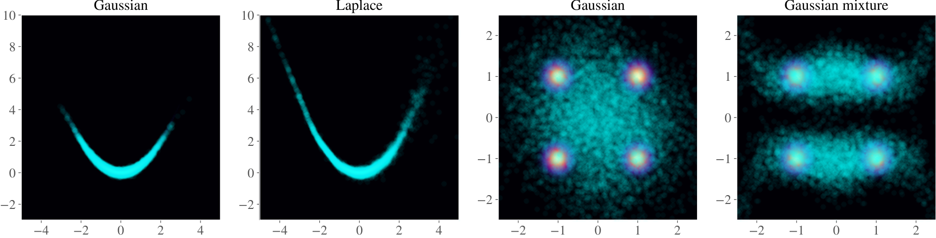
Looking at Figure 12, the heavier tails of the Laplace reference distribution resulted in heavier tailed output. Furthermore, the Gaussian mixture reference allowed the IAF two capture two modes, however it was unable to capture all four modes of the multimodal target. Results in Table 4 suggest it may be useful to consider the choice of as part of the optimisation problem to be solved, although we did not attempt to do so in this work.
C.5 Investigating the Choice of Lengthscale
In this section, we investigate how the choice of lengthscale of the inverse multi-quadric kernel (see Theorem 1) can affect the output of KSD-based measure transport. We will see that, relative to the target distribution, if is too small the resulting output can be too focused if the target distribution has a relatively large dispersion, and on the other hand, if is too large, the resulting output can exhibit pathologies. To demonstrate, we will focus on the NAF transport map and consider simple Gaussian targets with covariance matrices and . We will demonstrate the pathologies also occur in a more complex example of the multimodal problem encountered in Section 4.1. Output is shown in Figure 13.
The NAF used is the same one used in the experiments in Section 4.1 and specified in Section B.2. We used the Adam optimiser for iterations with learning rate .


C.6 Investigating the effect of input dimension in the ReLU network transport map
In this section we investigate how changing input dimension of the ReLU network transport map can effect output. In order to isolate the input dimension as our variable of investigation, we fix the topology of the ReLU and consider ReLU networks of the form
where , and are affine transformations and is the ReLU non-linearity, defined in Section A.4. We consider input dimensions . The target we considered is the multimodal target of Section 4.1. For each experiment, we pretrained each ReLU network on the reference distribution for iterations of Adam with learning rate . We then trained on the multimodal target for iterations of Adam, again with learning rate . Due to the random effects of initialisation (see Figure 15), we ran the experiments for different initialisations and report the best ones, see Table 5. The resulting transport maps are shown in Figure 14. As we can see, the transport map struggles with the multiple modes when the input dimension was or .
| Input dimension | |||||
|---|---|---|---|---|---|

C.7 Investigating the Effect of the U-statistic estimator vs. the V-statistic estimator
Recall from Equation 5, that the square of KSD is of the form
where is the density of . For a given I.I.D. sample from , there are two natural estimators of . The first is the V-statistic (KSD-V),
and the second is the U-statistic (KSD-U),
which is simply the V-statistic with the diagonal elements removed. The advantage of U-statistic is that it is unbiased and, for any given sample, provides the minimum-variance unbiased estimator (MVUE) [Liu et al. 2016]. On the other hand, the V-statistic provides a non-negative estimator, due to the positive-definiteness of .
To explore the differences between KSD-U and KSD-V as the objective, we re-ran the synthetic test bed experiments along with the majority of the transport maps in Section 4.1. Results are reported in Table 6. It appears that, although KSD-U and KSD-V often have very close outcomes, KSD-U seems to be strictly better than KSD-V. The transport maps and their initialisation were the same as was used in Section 4.1 and fully specified in Section B.2. For each experiment we used iterations of Adam with learning rate .
| Sinusoidal | Banana | Multimodal | |||||
|---|---|---|---|---|---|---|---|
| Transport Map | KSD-U | KSD-V | KSD-U | KSD-V | KSD-U | KSD-V | |
| IAF | 0.38 | 0.25 | 0.67 | ||||
| IAF (stable) | 0.35 | 0.36 | 0.19 | 0.61 | |||
| NAF | 0.55 | 0.58 | 0.43 | 0.095 | 0.12 | ||
| SAF | 0.23 | 0.27 | 0.48 | 0.30 | 1.2 | ||
| B-NAF | 0.78 | 0.85 | |||||
| Polynomial (cubic) | 0.40 | 0.61 | 0.51 | ||||
| IAF mixture | 0.39 | 0.040 | |||||
| ReLU network | 0.71 | 0.96 | 0.43 | 0.53 | 0.22 | 1.2 | |
C.8 Pathologies of KSD for Measure Transport
Since KSD is a score-based method, it may exhibit similar pathologies to other score-based methods; see e.g. Wenliang 2020. In this section, we detail certain pathologies of KSD-based measure transport that we found experimentally and, if available, offer potential mitigation strategies.
Point Convergence:
For small batch sizes (e.g. 25) in the sinusoidal synthetic experiment of Section 4.1, it was observed (albeit rarely) that, when using the ReLU transport map, the transport map converged to a limit in which all inputs were mapped to the origin. The origin is the mode of the sinusoidal synthetic density. This only occurred when using a degenerate initialisation and for small batch sizes. Due to the tightness of the sinusoidal target and the resulting large score values at points diverging away slightly from the support of the target, the KSD value of output for all the transport maps used in Section 4.1 was generally of the order . However, for the approximating transport map maps everything to the origin, the resulting KSD score was with . Thus, from the perspective of KSD, a transport map that maps everything to the origin and thus having poor Wasserstein distance, was considered better than transport maps that obtain smaller Wasserstein distances.
This problem was mitigated by using better initialisations, larger batch sizes and pretraining on the reference distribution.
Multimodal Failure:
It was found that, particularly with ReLU neural network transport map, the inferred transport map for the multimodal synthetic distribution in Section 4.1 could fail to find all four high density regions in the target. The outcome was highly dependent on the initialisation and even persisted when pretraining on the reference distribution. For example, in Figure 15 we plot three random initialisations of the ReLU transport map used in Section 4.1. Each transport map was pretrained on their reference distribution for iterations of Adam. The KSD estimates with using samples from the approximating distributions were , and from left to right respectively. The three outputs achieved broadly similar KSD scores, indicating that KSD was not able to differentiate between these outcomes. This is problem is further exacerbated as the number of modes of the target increases. For discussion of remedies, see Wenliang 2020.

Poor Choice of Lengthscale:
Finally, as we have seen in Section C.5, if the choice of is poor, the resulting output of KSD based measure transport can exhibit pathologies. This is demonstrated, for instance, in Figure 13. This issue is remedied by, for example, employing the median heuristic Garreau et al. 2018 to set the length-scale parameter in the kernel.