Computing planar shape and critical point evolution under curvature-driven flows

In geophysical applications there has been particularly keen interest in identifying shape descriptors which, on the one hand, can be reliably measured and, on the other hand, evolve in a monotonic manner under these flows. The latter property makes the time evolution invertible, enabling geophysicists to deduce the provenance of pebbles based on observation of their current shape [55].

One well-known and broadly applied shape descriptor is roundness, commonly identified by the isoperimetric quotient $Q=4\pi A/L^{2}$; here $A$ is the enclosed area and $L$ the length of its perimeter, that is, the total arclength of the curve $\Gamma$. The monotonicity of $Q(t)$ under 1 was proven by Gage [31]; Andrews [3] generalized this result to 4 and showed that the parameter value $\alpha=1/3$ (defining the affine shortening flow) separates flows with monotonically increasing and monotonically decreasing evolutions for $Q(t)$. We will illustrate these results in section 5.2, where we not only illustrate the monotonicity of $Q(t)$ but also that, depending on $\alpha$, it approaches nontrivial limits predicted by Andrews [6].

Roundness $Q$ is a classical geophysical shape descriptor which is relatively easily measured [55] and, as described above, displays monotonic evolution under 1. Still, it has a major handicap: under the Eikonal flow 2, which also serves as a relevant abrasion model in its own right, $Q(t)$ is decreasing monotonically [22], so the direction of its evolution is opposite to the evolution under purely curvature-driven abrasion. Hence, if both types of abrasion occur, the evolution of $Q(t)$ is unpredictable and unreliable.

To overcome the above difficulty, the (integer) number of critical points has been introduced [20, 25, 58] as a new type of shape descriptor. In this paper we will perform computations related to four alternative versions of critical points. In order to introduce them we first define some concepts and notation.

We can now list the four types of critical points whose trajectories we will investigate during evolution of a given curve under the Andrews-Bloore flow 5:

• $n_{\mbox{\tiny$O$}}(t)$

  denotes the number of critical points of $r(\varphi)=r_{\mbox{\tiny$O$}}(\varphi)$, characterized by $r^{\prime}=dr/d\varphi=0$, when the reference point $O$ is chosen arbitrarily and remains fixed throughout the evolution;
  

• $n_{\mbox{\tiny$C$}}(t)$

  denotes the number of critical points of $r(\varphi)=r_{\mbox{\tiny$C$}}(\varphi)$, characterized by $r^{\prime}=dr/d\varphi=0$, when the reference point is the centroid $C(t)$ during the evolution, the location of which is generally not fixed under the flow;
  

• $n_{\mbox{\tiny$U$}}(t$)

  denotes the number of critical points of $r(\varphi)=r_{\mbox{\tiny$U$}}(\varphi)$, characterized by $r^{\prime}=dr/d\varphi=0$, when the reference point is the ultimate point $U$ throughout the evolution;
  

• $n_{\kappa}(t)$

  denotes the number of critical points of $\kappa(\varphi)$ characterized by $d\kappa/d\varphi=0$; this number is independent of the chosen reference point for the periodic function $r$ used to compute the evolution.

In general, $n_{\mbox{\tiny$O$}}$ and $n_{\mbox{\tiny$U$}}$ have no direct physical meanings. On the other hand, $n_{\mbox{\tiny$C$}}$ is the number of static balance points of the homogeneous disk bounded by the curve $\Gamma$, rolling along its perimeter on a frictionless, horizontal surface.

In this paper we only treat the two-dimensional problem directly. However, we mention that the definitions are analogous in three dimension. In particular, static balance points of pebbles are easily determined either by hand experiments or by computer analysis of scanned image data. The most remarkable property of the different types of numbers of critical points above is that they appear to be decreasing monotonically (either in a deterministic or in a statistical sense) under all types of natural abrasion [20, 22]. The main goal of our paper is to demonstrate this general property. This motivated the numerical algorithm presented here, designed for the purpose of tracking critical points during curve evolution. It allows us, on the one hand, to illustrate rigorously proven results regarding the evolution of critical points and, on the other hand, to perform computations in support of specific conjectures. We proceed by providing an overview of both kinds of results.

We present in this paper a numerical method for computing the evolution under the flow 5 of a given curve in the plane — designed specifically to reliably track (the trajectories of) critical points along the evolution, all the way up to (very close to) the final point. We require that the initial curve admits polar coordinates from a point in its interior. Such curves are known as star-like, and $r(\varphi)$ is given as the distance from the reference point of the unique intersection point of the curve with the ray of angle $\varphi\in[-\pi,\pi]$. Note further that star-like curves are a natural generalisation of convex curves, and that the flow 5 generally preserves the star-like nature of the initial curve; in fact, it is typically the case that a star-like curve becomes convex under evolution.

The algorithm’s capability of tracking critical points of the radial distance function $r(\varphi)$ is achieved by representing $r(\varphi)$ by a piecewise polynomial (over a specified mesh). This is natural in light of our wish to study the functions $n_{\mbox{\tiny$O$}}(t)$, $n_{\mbox{\tiny$C$}}(t)$ and $n_{\mbox{\tiny$U$}}(t)$ of critical points, as determined by the chosen fixed or moving reference point, as well as the number of critical points $n_{\kappa}(t)$. The general setup of our method is quite flexible and allows for different types of meshes and remeshing strategies. The key property of our approach is that every curve during the evolution is represented by a sufficiently smooth function that can be evaluated for any angle, that is, anywhere along the curve and not just at the mesh points. Since our representation is polynomial, the derivatives of the radial distance function $r$, the normal and the curvature $\kappa$ at any point of the curve, as well as certain observables, can be computed symbolically, that is, do not need to be approximated by using numerical differentiation.

Indeed, we will demonstrate that, with appropriately chosen accuracy settings, our algorithm is able to track reliably and with manageable computational effort the critical points of the radial distance function $r$ and of the curvature $\kappa$ during evolutions of curves under 5, including for choices of the parameters $c$ and $\alpha$ beyond the standard case $c=0$ and $\alpha=1$ of the curve-shortening flow. It is this new capability that distinguishes our formulation from existing methods for computing curvature-dependent flows. Reaction-diffusion techniques [10], level-set method [49, 48, 54], and front-tracking methods based on finite differences [27, 44] and related finite element methods [11, 27, 42, 45] have been used for this purpose. These computational approaches are highly efficient in several situations. Generally, the focus has been on some particular property of the problem or application, such as the curve reaching a singularity and breaking up into a set of disconnected curves in the case of level set methods. Moreover, front-tracking methods, in particular, which may also feature different types of mesh adaptation [11, 44], can be used to visualize the evolution of curves (that need not be star-like or convex) under the curve-shortening flow 1; see, for example, the illustrations in [16] of results from [49, 43]. On the other hand, the evolution of shape descriptors, especially trajectories of critical points and their numbers $n_{\mbox{\tiny$O$}}(t_{\max})$ and $n_{\mbox{\tiny$C$}}(t_{\max})$, has not been the focus of computations before. At the early stages of this project, we found that the existing methods are not well suited to capturing the fine details of the curve required for this task: even with very fine meshes and/or extremely small time steps it is difficult to achieve and maintain the required accuracy as the final point is approached. The approach presented here is complementary to available methods and has been inspired by collocation methods for boundary value problems of differential equations [18, 36]. The underlying idea is to work with a space of smooth approximating functions [53, 57], generally piecewise polynomials, to represent the global objects under consideration such as periodic orbits of differential equations or curves or fronts evolving under a geometric flow. Another important aspect of our method is that the planar curve is represented by a function of a single variable, namely the periodic radial distance function $r$, whose critical points are therefore readily available. While this requires that any curve be star-like, this is actually quite a natural assumption in the context of abrasion problems and limiting shapes under curvature flows. A method that is quite similar in spirit is that for front propagation in the Navier-Stokes equations in [51], where the front is approximated with a parametric representation based on polynomials over a list of points; the front is then propagated by interpolating the velocity field over these points.

Section 2 first introduces the polar parameterization of a star-like curve and then details how all relevant quantities can be computed from its periodic radial distance function. We then discuss the beneficial properties of the central parameterization (with the centroid as the reference point) in 2.1, how symmetries of a curve are reflected in its polar parameterization in 2.2, and properties of trajectories of critical points in 2.3. Our computational method is then presented in 3, where we introduce the space of discretized curves in 3.1 and then formulate the general algorithm in 3.2; time stepping, the choice of mesh, its propagation and remeshing are discussed in 3.3 through 3.6, respectively. Section 4 then provides a number of benchmark test that demonstrate the effects of different accuracy settings: the mesh size in 4.1 and 4.2, and the type of mesh and the remeshing strategy in 4.3; we then show in 4.4 that trajectories of critical points can be computed reliably, irrespective of the position of the curve; the final 4.5 shows that an initial ellipse does indeed not change its shape (within the numerical accuracy of the computation) under the affine shortening flow, as required by a result of Andrews [4]. In 5 we then provide two case studies that demonstrate how our algorithm can be used as a tool for the experimental investigation of the evolution under 5 of different types of curves; in 5.1 we provide numerical evidence in support of 1 and 2. In the final 5.2 we illustrate results of Andrews regarding the shape evolution for $c=0$ and $0<\alpha\leq 1$ and investigate the limit shapes of curves with $D_{n}$-symmetry and with $C_{n}$-symmetry. In 6 we draw some conclusions and point to future work. Finally, A provides some additional background on the existence of a polar parameterization.

As we discussed in 2, the radial distance function $r=r_{\mbox{\tiny$O$}}$ for any choice of reference point $O$ contains all of the information on $\Gamma$. So in this sense, any reference point is as good as any other reference point. However, in the context of shape evolution it is a natural choice to use the center of gravity or centroid $C$ of the (homogeneous) shape or region bounded by $\Gamma$ as the reference point. The centroid is intrinsic to the curve and can be computed from any polar parameterization as

Here, $A$ is the area of the shape bounded by $\Gamma$, which is also intrinsic and given by

We refer to the specific polar parameterization with $O=C$ as the central parameterization and to the periodic function $r$ as the central radial distance function, which we denote $r_{\mbox{\tiny$C$}}$ where the context calls for it. The central parameterization has a number of advantages.

1. 1.

   The central parameterization encodes the relevant properties of $\Gamma$ in a particularly convenient way. Namely, the stationary points of the associated homogeneous shape are immediately available as the critical points of the central radial distance function $r_{\mbox{\tiny$C$}}$, as is the number of stationary points $n_{\mbox{\tiny$C$}}$; note that stationary points along negatively curved parts of $\Gamma$ need to be balanced ‘on a pin’; see A.
   

2. 2.

   For the central parameterization any discrete symmetries of the curve $\Gamma$ are conveniently represented as symmetires of the central radial distance function $r_{\mbox{\tiny$C$}}$; see 2.2 for details.
   

3. 3.

   The reference point $C$ is inherent to the curve $\Gamma$. Hence, the central parameterization, if it exists, is a well-defined and definite choice of polar parameterization, which is an advantage from the algorithmic point of view. We remark that the centroid $C$ is generally not fixed under curvature flow, but can be tracked as $C(t)$ at negligible extra cost by evaluating the integral 21; in particular, $C(t)$ converges to the ultimate points $U$ as $t\to t_{\max}$.
   

4. 4.

   Should information on the evolution of critical points of the radial distance function $r_{\mbox{\tiny$O$}}$ for any other reference point $O$ be required, it can be found from the central parameterization by post-processing; in other words, it is not necessary to recompute the evolution.
   

For these reasons we will work in the implementation of our algorithm for the evolution of curves under 5 with the central parameterization whenever it exists, that is, when the centroid can be chosen as a reference point; see also A. While this is not true in general, it is observed that for many choices of $c$ and $\alpha\geq 0$ the curvature flow 5 drives any star-like curve $\Gamma$ towards convexity. This has been proven by Grayson for $c=0$ and $\alpha=1$ [33] and by Andrews for certain intervals of $\alpha$ [7]. In fact, for all our examples the centroid $C$ can be chosen as a reference point, so that the central parameterization is already available for the initial curve $\Gamma$.

We will also consider evolutions of curves that are invariant under a discrete symmetry group; typically, this will be the dihedral group $D_{n}$ of rotations and reflections of a regular $n$-gon in $\mathbb{R}^{2}$. So suppose that $\Gamma$ is invariant under the discrete group $G$, which means that $g\Gamma=\Gamma$ for all $g\in G$; here $g$ acts on $\Gamma$ as either a rotation or a reflection of $\mathbb{R}^{2}$. The question is whether these intrinsic symmetries of $\Gamma$ given by $G$ are reflected in the radial distance function $r_{\mbox{\tiny$O$}}$ of the polar parameterization with a given reference point $O$. This is only the case when $O$ is chosen to lie in the fixed point subspace of the respective group element or subgroup. More specifically, suppose $O\in{\rm Fix}(H)$ for some subgroup $H\leq G$, then $H$ induces an invariance of the scalar function $r_{\mbox{\tiny$O$}}$, namely

for a rotation over $\frac{2\pi}{\ell}$ about $O$ and

for a reflection in a line through $O$ of angle $\theta$. Hence, if $O\in{\rm Fix}(G)$ then $r=r_{\mbox{\tiny$O$}}$ has all symmetries represented by $G$; indeed then $r_{\mbox{\tiny$O$}}^{\prime}$ and $r_{\mbox{\tiny$O$}}^{\prime\prime}$ have the exact same symmetries of translation and reflection (in the exact same points). Note that the tangent $\mathbf{n}$ and the signed curvature $\kappa$ do not depend on the choice of reference point; hence, these periodic function of $\varphi$ are $G$-invariant in the same way (that is, under discrete translations and reflections) in any case.

The centroid $C$ of $\Gamma$ is fixed under all elements of $G$, that is, $C\in{\rm Fix}(G)$, so that the radial distance function $r_{\mbox{\tiny$C$}}$ has all symmetries of $G$. Moreover, unless $G=\mathbb{Z}_{2}$ is generated by a single reflection, $G$ contains a rotation, which must therefore be a rotation of $\Gamma$ around $C$. In particular, $C$ lies on the intersection of all lines of reflection. Note that the normal $\mathbf{n}(\theta)$ of a point $\gamma(\theta)$ on a line of reflection points to $C$; hence, generically, $r_{\mbox{\tiny$C$}}$ has a maximum or minimum, reflecting the fact that every point of $\Gamma$ on a line of reflection is a stationary point. It follows from 19 that the scalar function $\kappa$ has the same symmetry as $r_{\mbox{\tiny$C$}}$, which means that the stationary points on lines of reflection are also extrema of the curvature $\kappa$. The center $I$ of the largest inscribed circle must also be fixed under the action of the group. It follows that, if the group $G$ contains two reflections or a rotation, then $I=C$ and the extrema of the curvature $\kappa$ coincide with the stationary points.

Considering curves with discrete symmetry is interesting because the flow of 5 preserves symmetry; this follows from the fact that the normal and the curvature inherit the symmetry of $\Gamma$. Hence, for any $0\leq t<t_{\max}$ the curve $\Gamma(t)$ is invariant under the symmetry group $G$ of $\Gamma$; we will see examples of this in the coming sections. In particular, any method to compute the evolution of a planar curve must preserve its symmetry. As we will see in 3, checking this property provides a good test of the performance of our implementation. Indeed, whether symmetry is preserved can be checked readily by considering the symmetry properties of the radial distance function $r_{\mbox{\tiny$C$}}$ under evolution. This is another reason why the central parameterization is a good choice of parameterization to work with algorithmically.

The flow of equation 5 for given $c$ and $\alpha$ generates the (forward) evolution $\Gamma(t)$ of a given curve $\Gamma=\Gamma(0)$. We consider here only evolutions of star-like curves and compute the evolution $\Gamma(t)$ for $0\leq t\leq t_{\max}$ via the corresponding radial distance distance functions $r(\varphi;t)$ of its polar (and generally central) parameterization. For any $t$, the function $r(\varphi;t)$ is a periodic Morse function [9, 17, 52], which means (assuming that $\Gamma(t)$ is sufficiently smooth) that the derivative $r^{\prime}(\varphi;t)=\frac{dr}{d\varphi}(\varphi;t)$ vanishes at isolated points $\varphi^{*}=\varphi^{*}(t)\in[-\pi,\pi]$. Generically, these points correspond to an alternating sequence of maxima and minima separated by isolated roots of the second derivative $r^{\prime\prime}(\varphi;t)=\frac{d^{2}r}{d\varphi^{2}}(\varphi;t)$; due to periodicity, there are generically equal numbers of maxima and minima, that is, an even number of extrema of $r(\varphi;t)$. It follows further from singularity theory [9, 17, 32, 52] that the number of extrema changes generically at isolated points of the $t$-line. Namely, at such a point $t^{*}$ one has either

1. 1.

   In the absence of additional symmetry properties of $\Gamma(t)$: a fold bifurcation at $t^{*}$, which is a cubic singularity where $\frac{dr}{d\varphi}(\varphi^{*};t^{*})=\frac{d^{2}r}{d\varphi^{2}}(\varphi^{*};t^{*})=0$; the genericity condition is that $\frac{d^{3}r}{d\varphi^{3}}(\varphi^{*};t^{*})\neq 0$. In this bifurcation a maximum and a minimum of $r$ disappear or appear as $t$ increases through $t^{*}$.
   

2. 2.

   Across a line of reflection of $\Gamma(t)$: a pitchfork bifurcation at $t^{*}$ of an extremum of $r(\varphi^{*};t^{*})$, where $\frac{dr}{d\varphi}(\varphi^{*};t^{*})=\frac{d^{3}r}{d\varphi^{3}}(\varphi^{*};t^{*})=0$; here the genericity condition is that $\frac{d^{5}r}{d\varphi^{5}}(\varphi^{*};t^{*})\neq 0$, and note that $r$ is an odd function with respect to $\varphi^{*}+\varphi$ due to reflectional symmetry. In this bifurcation a pair of minima/maxima off the reflection axis disappear or appear by meeting a maximum/minimum on the axis of reflection as $t$ increases through $t^{*}$.
   

3. 3.

   With rotational symmetry of $\Gamma(t)$: a fold or pitchfork bifurcation at $t^{*}$ occurs simultaneously along the orbit of the generator of rotation, that is, for all $\frac{2\pi}{\ell}\varphi^{*}$ where $\ell$ is the order of the rotational subgroup of the symmetry group $G$ of $\Gamma(0)$.
   

The exact same statements hold also for the scalar signed curvature function $\kappa(\varphi;t)$ of $\Gamma(t)$, which is also a periodic Morse function determined from $r(\varphi;t)$ by 19. Since 5 preserves symmetry, it follow that the numbers $n_{\mbox{\tiny$O$}}(t)$, $n_{\mbox{\tiny$C$}}(t)$, $n_{\mbox{\tiny$U$}}(t)$ and $n_{\kappa}(t)$ are generically constant and even, and change at isolated points $t^{*}$ by $2\ell$ where $\ell$ is the order of the rotation subgroup of the symmetry group of $\Gamma=\Gamma(0)$ (which may be empty, in which case $\ell=1$).

The challenge, from both the theoretical and the algorithmic point of view, is to accurately compute the trajectories of the different types of critical points during the evolution of a given curve $\Gamma$. The numerical method we introduce below is specifically designed for this task. In particular, it allows us to illustrate, confirm or make statements about the properties of the numbers $n_{\mbox{\tiny$O$}}(t)$, $n_{\mbox{\tiny$C$}}(t)$, $n_{\mbox{\tiny$U$}}(t)$ and $n_{\kappa}(t)$ as $t\to t_{\max}$.

We first deal with the issue that curves in $\mathbb{R}^{2}$ are infinite-dimensional objects. Hence, the task is to discretize any star-like curve $\Gamma$ in an appropriate way. To achieve this we consider a finite-dimensional space $\mathscr{D}$ of discretized curves that are defined over a mesh of $N$ points. There are several choices one could make for the mesh and the space of functions that specify $\mathscr{D}$. We work here with a mesh

of mesh points $m_{j}$ on the given curve $\Gamma$. Since $\Gamma$ has a given polar parameterization $\gamma$, the mesh $M$ can be pulled back to a mesh

of the polar angle $\varphi$. Reversely, for a polar-angle mesh $M_{\varphi}$ the parameterization $\gamma$ induces a unique mesh of points on $\Gamma$, and we express this relationship between the two dual meshes as

for notational convenience.

We now consider piecewise polynomial radial distance functions through the points of the polar-angle mesh $M^{\varphi}$. Again, there are different options for choosing such polynomials. We define and compute them here as interpolating polynomials of degree $p$ on each mesh interval $[\varphi_{i},\varphi_{i+1}]$, whose first $p$ derivatives agree at the mesh points of $M^{\varphi}$. We refer to this class of periodic piecewise polynomial functions as $\mathscr{P}_{N}^{p}$; they are also known as periodic splines of degree $p$ [1]. This choice defines the discretization space

Here $N_{\max}$ and $p$ are taken to be fixed; we find that degree $p=5$ polynomials are a suitable choice, in practice, in terms of the balance between providing sufficient smoothness versus the cost of computing the polynomial representation. Similarly, there is a trade-off between run-time and data size versus accuracy when it comes to the choice of the mesh size. Note that we require that the mesh size $N$ remains bounded by some apriori bound $N_{\max}$ solely to ensure that $\mathscr{D}$ is of finite dimension; hence, our setup allows for the adaptation of the mesh and its size during the computation of an evolution. We find that meshes of $N$ between 50 and 100 generally suffice for the curves we consider; see section 4 for further details.

It is important to note that the radial distance function $r(\varphi)$ of any curve $\Gamma\in\mathscr{D}$ is defined for all $\varphi\in[-\pi,\pi]$. In other words, we are still working on a space of periodic functions and not just on a set of mesh points. In particular, the derivatives $r^{\prime}$ and $r^{\prime\prime}$, as well as the normal $\mathbf{n}$ and curvature $\kappa$ are also piecewise polynomial functions, which can be computed symbolically from $r\in\mathscr{P}_{N_{\max}}^{p}$. Hence, all of these periodic functions can be evaluated exactly at any point $\varphi\in[-\pi,\pi]$.

Any curve star-like curve $\Gamma$ is restricted to the discretization space $\mathscr{D}$ in a unique way by the choice of the mesh $M$ (and the reference point); we refer to this restriction or projection to the curve with the corresponding radial distance function $r\in\mathscr{P}_{N_{\max}}^{p}$ as $\Pi_{M}(\Gamma)$ for notational convenience. Note that the piecewise polynomial radial distance function $r$ of the projected curve $\Pi_{M}(\Gamma)\in\mathscr{D}$ can be computed readily for any chosen mesh and reference point; in what follows, the reference point is always the centroid C unless otherwise stated.

For a curve $\Gamma\in\mathscr{D}$ with a central parameterization $\gamma$ with piecewise polynomial radial distance function $r\in\mathscr{P}_{N_{\max}}^{p}$ for some given mesh $M$ we perform the integration with an Euler step $E_{h}$ of stepsize $h$ for the flow of 5 given by

where

The resulting, $h$-evolved periodic orbit $\Gamma_{h}=E_{h}(\Gamma)$ is, in general, not in the discretization space $\mathscr{D}$, that is, it does not have a polar parameterization with a piecewise polynomial radial distance function. This problem is overcome by constructing the new and unique radial distance function $r_{h}\in\mathscr{P}_{N_{\max}}^{p}$ and associated parameterization $\gamma_{h}(\varphi)$ with respect to a prespecified mesh $\widehat{M}\subset E_{h}(\Gamma)$ (and given reference point). Formally, this is the projection $\Pi_{\widehat{M}}$ from $\mathscr{C}$ back to $\mathscr{D}$, which can be expressed as

Therefore, the integration step on the discretization space $\mathscr{D}$ of a curve $\Gamma\in\mathscr{D}$ is defined as an Euler step followed by projection back onto $\mathscr{D}$, that is, by $\Pi_{\widehat{M}}(E_{h}(\Gamma))\subset\mathscr{D}$; note that this requires one to specify the mesh $\widehat{M}$ used in the restriction back to $\mathscr{D}$.

The evolution algorithm to approximate the evolution $\Gamma(t)$ of a given star-like curve $\Gamma$ under the flow of 5 now consists of computing a sequence $(\Gamma_{i})_{0\leq i\leq I}\subset\mathscr{D}$ as

By construction, the parameterizations

have central radial distance functions $r_{i}$ that are piecewise interpolating polynomials defined by the meshes $M_{i}$. Where it is appropriate to stress that the sequence $(\Gamma_{i})$ represents a time evolution, we also refer to $\Gamma_{i}$ as $(\Gamma_{t_{i}})$, where $t_{i}=\sum_{l=1}^{i}h_{l}$ is the integration time up to step $i$ of the computation.

Formulating the evolution algorithm in general terms first is convenient because it encompasses different strategies for updating the mesh, that is, the discretization of the curve that is being evolved. In the remainder of this section, we present our numerical implementation of the general evolution algorithm given by 32. To this end, we will specify: (1) the stepsize sequence $(h_{i})$ with suitable stopping criteria for the computation, and (2) a strategy for choosing the mesh $(M_{i})$ at step $i$ of the computation. We will then evaluate in 4 with a number of test-case examples how the accuracy of a computed evolution can be ensured by selecting suitable values of the different accuracy parameters, including the integration stepsize, the mesh size and the remeshing frequency.

The overall or average curvature of the curve increases during an evolution as time $t$ converges to $t_{\max}<\infty$. This is why we determine the stepsize at step $i$ from the curvature as

Here the accuracy parameter $S$ determines the fineness of the stepsize sequence $(h_{i})$; it is chosen at the start of a computation and then remains constant. The computation stops when the time step $h_{i}$ drops below a pre-specified minimum $h_{\rm min}$.

During an evolution where the curve reaches a final point in $\mathbb{R}^{2}$ the radial distance function $r_{i}$ converges with $i$ to the constant function $0$; this also means that the area $A_{i}$ of $\Gamma_{i}$ goes to zero. Moreover, the average of the absolute value of the curvature $|\kappa_{i}|$ grows beyond bound. Working with too small $r_{i}$ or too large $|\kappa_{i}|$ is not practical numerically, which is why we limit their ranges; note that very small $r_{i}$ or $A_{i}$ or very large curvature indicates that the total integration time $t_{i}=\sum_{l=1}^{i}h_{l}$ is close to $t_{\max}$. This is formalized in the following list of stopping criteria for the computation.

• (i)

  $h_{i}<h_{\rm min}$;

• (ii)

  $\mathrm{Var}(r_{i+1})<1e^{-8}$;

• (iii)

  $A_{i}<A_{min}$;

• (iv)

  $\mathrm{max}_{\varphi\in[-\pi,\pi]}(|\kappa_{i}|/\mathrm{Avg}(r_{i})<1e^{-5}$.
  

Note that we impose global limits on the radial distance function $r_{i}$ and the curvature $\kappa_{i}$, while $h_{\rm min}$ and $A_{min}$ are accuracy parameters of the algorithm. The computation stops as soon as one of these stopping criteria is satisfied.

There are two types of uniform meshes that we consider as part of our implementation: meshes that are uniform in the phase $\varphi$, and meshes that are uniform in arclength $s$. We will use either as appropriate for the initial mesh $M_{0}$, as well as for remeshing during a computation.

A phase-uniform mesh $M$ for a star-like curve $\Gamma$ with polar parameterization $\gamma$ is given by

Phase-uniform meshes are computationally inexpensive to generate and their uniformity in $\varphi_{j}$ is an advantage for the construction of the piecewise polynomial periodic function $r$ of the associated discretization $\Pi_{M}(\Gamma)\in\mathscr{D}$. Figure 1 shows the phase-uniform mesh of size $N=20$ for our standard example curve, defined in 38 below, which generates the piecewise polynomial functions $r$, $r^{\prime}$ and $r^{\prime\prime}$ of its discretization in $\mathscr{D}$. Note that the mesh points on $\Gamma$ are distributed almost uniformly in arclength as well. This is the case for any curve that is reasonably close to being circular, which is why, as we will see in 5, phase-uniform meshes are a suitable choice for such curves.

An arclength-uniform mesh $M$ for $\Gamma$, on the other hand, is given by

here $\tilde{\gamma}$ is the associated arclength parameterization of $\gamma$ given by 9. By construction, the mesh points $m_{j}$ are uniformly distributed in arclength along $\Gamma$, while the corresponding phases $\varphi_{j}\in M^{\varphi}$ are not uniformly distributed in $[-\pi,\pi]$. Working with arclength-uniform meshes is more computationally expensive but, as we will see in 5, may be required for the accurate computation of the evolutions of certain curves, in particular of ellipses.

Figure 2 illustrates the difference between the two types of uniform meshes with the example of a mesh of size $N=20$ on an ellipse of axis ratio 2, the standard ellipse 39 with $a=1$ and $b=0.5$. The uniform mesh $M^{\varphi}$ generates a radial distance function $r$ in panel (a1) with interpolated points that are at fixed distance $\frac{2\pi}{N}$. The associated meshpoints of the dual mesh $M$ on the ellipse in panel (a2) are concentrated near the minima of the curvature and clearly not at equal arclengths from each other. For the arclength-uniform mesh the situation is reversed: the uniformity of the points of the mesh $M$ on the ellipse in panel (b2) generates a non-uniformity of the associated interpolation points of $M^{\varphi}$ that define the radial distance function $r$ in panel (b1). Observe how points in $M^{\varphi}$ now concentrate near phase angles corresponding to points of high curvature of the ellipse. Note that there is no distinguishable difference on the level of Figure 2 between the two radial distance functions and the two respective approximate ellipses; the accuracy of approximation for either uniform parameterization will be considered in more detail in 4.

Any computation of an evolution of any star-like curve $\Gamma$ starts with the choice of the initial mesh $M_{0}$ of size $N$ that then generates the piecewise polynomial central radial distance function $r_{0}$ that gives the parameterization of the initial curve $\Gamma_{0}=\Pi_{M_{0}}(\Gamma)\in\mathscr{D}$. Throughout, we take $M_{0}$ to be a uniform mesh in either phase or arclength, depending on the situation; here $N$ is chosen sufficiently large to ensure that the errors between the respective periodic functions and their derivatives of $\Gamma$ and $\Gamma_{0}$ are sufficiently small; see 4.

To compute the new radial distance function $r_{i}$ at step $i$ one needs to specify the new mesh $M_{i}$ on the curve $E_{h_{i}}(\gamma^{i-1})$. The most straightforward way to obtain $M_{i}$ is to push forward or propagate the mesh $M_{i-1}$ under the Euler step 29. This means that $M_{i}=E_{h_{i}}(M_{i-1})$, which is computed as

here $\varphi_{i-1,j}\in M^{\varphi}_{i-1}=\gamma^{-1}_{i-1}(M_{i-1})$ is the associated phase of the mesh point $m_{i-1,j}\in M_{i-1}$.

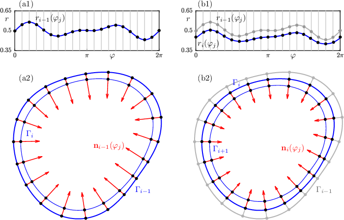
This choice of propagating the mesh at each step gives the mesh propagation implementation of the general algorithm, which forms the core of our method. It has the advantage that all that is required computationally at each integration step is calculating the $N$ Euler steps at each mesh point, followed by the subsequent construction of the piecewise polynomial radial distance functions $r_{i}$. This is illustrated in Figure 3, which shows steps $i$ and $i+1$ of the mesh propagation implementation. The piecewise polynomial radial distance function $r_{i-1}$ in panel (a1) generates both the curve $\Gamma_{i-1}$ via its parameterization $\gamma_{i-1}(\varphi)$ as well as the normals $\mathbf{n}_{i-1}$ at the mesh $M_{i-1}$ in panel (a2). The propagated mesh is the result of Euler steps at each mesh point, and it defines the piecewise polynomial radial distance function $r_{i}$ in Figure 3 (b1). The corresponding parameterization $\gamma_{i}(\varphi)$ and normals $\mathbf{n}_{i}$ at the mesh points in panel (b2) then give the next curve with parameterization $\gamma_{i+1}(\varphi)$. Note that during each step of the computation there is a continuous switching between the two representations of the curve — in the sense that we are using both the mesh of points on the respective curve, as well as the dual phase-mesh that defines the piecewise polynomial radial distance function needed to evaluate the normals and the curvature.

During mesh evolution the mesh points tend to drift towards points of higher curvature of the curve. This effect is quite limited when the variation in curvature is small, but can be substantial when it is larger. Rather than countering this with an increase of the overall mesh size $N$, it is more efficient to perform remeshing at suitable steps of the evolution algorithm. This can be done in a straightforward way at step $i$ because the radial distance function $r_{i}$ and the parameterization $\gamma_{i}$ are functions that can be evaluated at any value of $\varphi\in[-\pi,\pi]$. Hence, remeshing simply consists of taking a uniform mesh $M^{*}\subset\Gamma_{i}$, either phase-uniform or arclength uniform, and computing the radial distance function defined by $M^{*}$. The result is the remeshed piecewise polynomial radial distance function $r_{i}^{*}$ with parameterization $\gamma^{*}_{i}$ of the reparameterized curve $\Gamma^{*}_{i}$.

Remeshing requires the construction of the uniform mesh $M^{*}$ and the subsequent construction of the new radial distance function $r_{i}^{*}$, so adds to the computational effort. On the other hand, it allows one to work with meshes of smaller size $N$. There is clearly a balance in terms of computational effort and accuracy, when deciding on a remeshing frequency versus taking larger $N$. We also remark that it may be advantageous to increase or reduce the mesh size $N$ when remeshing.

The overall evolution algorithm as implemented, with mesh propagation and remeshing when required, is presented in schematic form as Algorithm 1. This formulation is for a general reference point $O_{i}$ at every step, but we stress once more that we are using the centroid $C_{i}$ as the reference point whenever it is available.

References

- [1] J. Ahlberg, E. Nilson, and J. Walsh. The Theory of Splines and Their Applications. Elsevier BV, 1967.
- [2] L. Alvarez, F. Guichard, P.-L. Lions, and J.-M. Morel. Axioms and fundamental equations of image processing. Archive for Rational Mechanics and Analysis, 123:199–257, 1993.
- [3] B. Andrews. Contraction of convex hypersurfaces in Euclidean space. Calculus of Variations and Partial Differential Equations, 2(2):151–171, 1994.
- [4] B. Andrews. Contraction of convex hypersurfaces by their affine normal. Journal of Differential Geometry, 43(2):207–230, 1996.
- [5] B. Andrews. Evolving convex curves. Calculus of Variations and Partial Differential Equations, 7(4):315–371, nov 1998.
- [6] B. Andrews. Classification of limiting shapes for isotropic curve flows. Journal of the American Mathematical Society, 16(02):443–460, dec 2002.
- [7] B. Andrews. Non-convergence and instability in the asymptotic behaviour of curves evolving by curvature. Communications in Analysis and Geometry, 10(2):409–449, 2002.
- [8] B. Andrews and M. Feldman. Nonlocal geometric expansion of convex planar curves. Journal of Differential Equations, 182(2):298–343, 2002.
- [9] V. I. Arnold. Singularity Theory. Cambridge University Press, 2013.
- [10] J. Barrett, K. Deckelnick, and V. Styles. Numerical analysis for a system coupling curve evolution to reaction diffusion on the curve. SIAM Journal on Numerical Analysis, 55(2):1080–1100, 2017.
- [11] J. W. Barrett, H. Garcke, and R. Nürnberg. The approximation of planar evolution by stable fully implicit finite element schemes that equidistribute. Numerical Methods for Partial Differential Equations, 27:1–30, 2011.
- [12] F. J. Bloore. The shape of pebbles. Journal of the International Association for Mathematical Geology, 9(2):113–122, Apr 1977.
- [13] J. W. Bruce, P. J. Giblin, and C. G. Gibson. On caustics of plane curves. Amercan Mathematical Monthly, 88:651–667, 1981.
- [14] R. L. Bryant and P. A. Griffiths. Characteristic cohomology of differential systems II: Conservation laws for a class of parabolic equations. Duke Mathematical Journal, 78(3):531–676, June 1995.
- [15] B. Chow. On Harnack’s inequailty and entropy for the Gaussian curvature flow. Communications in Pure and Applied Mathematics, XLIV:469–483, 1991.
- [16] P. Daskalopoulos and N. Sesum. Ancient solutions to geometric flows. Notices of the American Mathematical Society, 67(04):1, Apr. 2020.
- [17] M. Demazure. Bifurcations and Catastrophes: Geometry of Solutions to Nonlinear Problems. Springer Berlin Heidelberg, 2000.
- [18] E. J. Doedel. Lecture notes on numerical analysis of nonlinear equations. In B. Krauskopf, H. M. Osinga, and J. Galán-Vioque, editors, Numerical Continuation Methods for Dynamical Systems: Path Following and Boundary Value Problems, pages 1–49. Springer Berlin Heidelberg, 2007.
- [19] G. Domokos. Monotonicity of spatial critical points evolving under curvature-driven flows. Journal of Nonlinear Science, 25(2):247–275, apr 2015.
- [20] G. Domokos. Natural numbers, natural shapes. Axiomathes, 2019.
- [21] G. Domokos and G. W. Gibbons. The evolution of pebble size and shape in space and time. Proceedings of the Royal Society of London A, 2012.
- [22] G. Domokos and Z. Lángi. The isoperimetric quotient of a convex body decreases monotonically under the Eikonal abrasion model. Mathematika, 65(1):119 – 129, 2019.
- [23] G. Domokos, Z. Lángi, and A. A. Sipos. Tracking critical points on evolving curves and surfaces. Experimental Mathematics, pages 1–20, Mar. 2019.
- [24] G. Domokos, J. Papadopulos, and A. Ruina. Static equilibria of planar, rigid bodies: is there anything new? Journal of Elasticity, 36(1):59–66, 1994.
- [25] G. Domokos, A. Á. Sipos, T. Szabó, and P. Várkonyi. Pebbles, shapes and equilibria. Mathematical Geosciences, 42:9, 2010.
- [26] T. A. Driscoll, N. Hale, and L. N. Trefethen. Chebfun Guide. Pafnuty Publications, Oxford, 2014.
- [27] G. Dziuk. Discrete anisotropic curve shortening flow. SIAM Journal on Numerical Analysis, 36(6):1808–1830, 1999.
- [28] D. L. Fidal and P. J. Giblin. Generic one-parameter families of caustics in the plane. Mathematical Procedings of the Cambridge Philosophical Society, 96:425–432, 1984.
- [29] W. J. Firey. Shapes of worn stones. Mathematika, 21(1):1–11, 1974.
- [30] M. Gage and R. S. Hamilton. The heat equation shrinking convex plane curves. Journal of Differential Geometry, 23(1):69–96, 1986.
- [31] M. E. Gage. Curve shortening makes convex curves circular. Inventiones Mathematicae, 76(2):357–364, 1984.
- [32] M. Golubitsky and D. Schaeffer. Singularities and Groups in Bifurcation Theory, Volume I. Springer Berlin Heidelberg, 1985.
- [33] M. A. Grayson. The heat equation shrinks embedded plane curves to round points. Journal of Differential Geometry, 26(2):285–314, 1987.
- [34] R. Hamilton. Three-manifolds with positive Ricci curvature. Journal of Differential Geometry, 17:255–306, 1982.
- [35] G. Huisken. Flow by mean curvature of convex surfaces into spheres. Journal of Differential Geometry, 20:237–266, 1984.
- [36] A. Iserles. A First Course in the Numerical Analysis of Differential Equations. Cambridge University Press, Cambridge New York, 1996.
- [37] T. Ishiwata and T. Ohtsuka. Evolution of a spiral-shaped polygonal curve by the crystalline curvature flow with a pinned tip. Discrete & Continuous Dynamical Systems - B, 22(11):1–35, 2017.
- [38] M. Kardar, G. Parisi, and Y.-C. Zhang. Dynamic scaling of growing interfaces. Physical Review Letters, 56:889–892, 1986.
- [39] A. Kneser. Bemerkungen über die Anzahl der Extrema der Krümmung auf geschlossenen Kurven und über verwandte Fragen in einer nicht euklidischen Geometrie. In Festschrift Heinrich Weber, pages 170–180. Teubner, 1912.
- [40] J. Koenderink. The structure of images. Biological Cybernetics, 50:363–370, 1984.
- [41] C. Lu, Y. Cao, and D. Mumford. Surface evolution under curvature flows. Journal Visual Communication and Imgage Representation, 13:65–81, 2002.
- [42] G. MacDonald, J. A. Mackenzie, M. Nolan, and R. Insall. A computational method for the coupled solution of reaction-diffusion equations on evolving domains and manifolds: Application to a model of cell migration and chemotaxis. Journal of Computational Physics, 309:207–226, 2016.
- [43] R. Malladi and J. A. Sethian. Level set methods for curvature flow, image enchancement, and shape recovery in medical images. In Visualization and Mathematics, pages 329–345. Springer Berlin Heidelberg, 1997.
- [44] J. A. Mckenzie, M. Nolan, C. F. Rowlatt, and R. H. Insall. An adaptive moving mesh method for forced curve shortening flow. SIAM Journal on Scientific Computing, 41(2):A1170–A1200, 2019.
- [45] K. Mikula and D. Ševčovič. Solution of nonlinearly curvature driven evolution of plane curves. Applied Numerical Mathematics, 31(2):191 – 207, 1999.
- [46] F. Mokhtarian, S. Abbasi, and J. Kittler. Efficient and robust retrieval by shape content through curvature scale space. In International Workshop on Image Databases and Multimedia Search, pages 35–42, 1996.
- [47] F. Mokhtarian and R. Suomela. Robust image corner detection through curvature scale space. IEEE Transactions on Pattern Analysis and Machine Intelligence, 20(12):1376–1381, Dec 1998.
- [48] S. J. Osher and R. P. Fedkiw. Level Set Methods and Dynamic Implicit Surfaces. Springer Berlin Heidelberg, 2002.
- [49] S. J. Osher and J. A. Sethian. Fronts propagating with curvature-dependent speed: Algorithms based on Hamilton-Jacobi formulations. Journal of Computational Physics, 79(1):12–49, Nov. 1988.
- [50] G. Perelman. Ricci flow with surgery on three-manifolds. http://arXiv.org/math.DG/0303109v1, 2003.
- [51] S. Popinet and S. Zaleski. A front-tracking algorithm for accurate representation of surface tension. International Journal for Numerical Methods in Fluids, 30(6):775–793, 1999.
- [52] T. Poston and I. Stewart. Catastrophe Theory and its Applications. Dover Publications, Mineola, N.Y, 1996.
- [53] T. Rivlin. An Introduction to the Approximation of Functions. Dover, New York, 1981.
- [54] J. A. Sethian. Level Set Methods and Fast Marching Methods: Evolving Interfaces in Computational Geometry, Fluid Mechnics, Computer Vision and Materials Science. Cambridge University Press, 1999.
- [55] T. Szabó, G. Domokos, J. P. Grotzinger, and D. J. Jerolmack. Reconstructing the transport history of pebbles on Mars. Nature Communications, 6:8366, 2015.
- [56] A. Townsend, H. Wilber, and G. B. Wright. Computing with functions in spherical and polar geometries i. the sphere. SIAM Journal on Scientific Computing, 2016.
- [57] L. N. Trefethen. Approximation Theory and Approximation Practice. SIAM, Philadelphia, 2013.
- [58] P. Várkonyi and G. Domokos. Static equilibria of rigid bodies: Dice, pebbles, and the Poincaré-Hopf theorem. Journal of Nonlinear Science, 16(3):255–281, May 2006.
- [59] G. B. Wright, M. Javed, H. Montanelli, and L. N. Trefethen. Extension of Chebfun to periodic functions. SIAM Journal on Scientific Computing, 2015.