Effective action for delta potentials: spacetime-dependent inhomogeneities and Casimir self-energy

As a warm-up, let us begin by considering the operator

(5)

$\displaystyle\Delta_{\delta}:=-\partial^{2}_{x}+\zeta\,\delta(x-L),\quad x\in\mathbb{R},$

for a constant $\zeta>0$ (as long as the contrary is not stated, this assumption will be considered throughout the rest of the article). Up to our knowledge, its exact HK has been obtained for the first time in [30] by considering path integral and Laplace-transform techniques; later, it was independently rederived in [31], in a similar way (employing methods of Brownian motion and Laplace transforms). Here we will provide a new derivation of an exact expression for its HK, which involves solving an integral equation derived from a path integral representation.

Recall that the problem of finding the HK of $\Delta_{\delta}$ is equivalent to the determination of the propagator of a particle in a first-quantization realm and subject to a potential which is a Dirac delta, to wit

(6)

$\displaystyle K_{\delta}(x,y;T):$

$\displaystyle=\int_{\begin{subarray}{c}q(0)=x\end{subarray}}^{q(T)=y}\mathcal{D}q(t)e^{-S_{\delta}},$

where

(7)

$\displaystyle S_{\delta}=\int_{0}^{T}dt\,\left[\frac{\dot{q}^{2}(t)}{4}+\zeta\,\delta(q(t)-L)\right].$

Notice, of course, that this corresponds to a ficticious particle that evolves in time $t$, which is ficticious as well. This implementation of path integrals in the computation of HKs and effective actions is usually called Worldline Formalism or String-inspired Formalism in the literature [29, 32]. In relation to Dirac delta potentials, a first-order perturbative computation of the Casimir energy between two semitransparent layers has been computed in [5], while other recent applications include computations in QED [33] and noncommutative Quantum Field Theory [34].

Coming back to Eq.(6), one can formally perform the usual expansion in powers of $\zeta$, which after choosing a convenient ordering in the intermediate times $t_{i}$ leads to

(8)

$\displaystyle\begin{split}K_{\delta}(x,y;T)&=\sum_{n=0}^{\infty}(-\zeta)^{n}\int_{0}^{T}dt_{n}\int_{0}^{t_{n}}dt_{n-1}\cdots\int_{0}^{t_{2}}dt_{1}K_{0}(y,L;T-t_{n})\\ &\hskip 42.67912pt\times K_{0}(L,L;t_{n}-t_{n-1})\cdots K_{0}(L,L;t_{2}-t_{1})K_{0}(L,x;t_{1}),\end{split}$

where $K_{0}$, the free HK, has the expression

(9)

$\displaystyle K_{0}(x,y;T):=\frac{e^{-\frac{(x-y)^{2}}{4T}}}{\sqrt{4\pi T}}.$

From Eq. (8), one can show that the HK satisfies an integral equation whose kernel is nothing but the HK of the free particle [35]. This last fact obstructs the obtention of the solution via iterated kernels and one then needs to recur to Laplace-transform techniques.

However, one may also derive from Eq.(8) a simpler integral equation. In order to do so, we perform a change of variables $s_{1}:=t_{1}\,s_{2}:=t_{2}-t_{1},\,s_{3}:=t_{3}-t_{2},$ etc., and obtain

(10)

$\displaystyle K_{\delta}(x,y;T)$

$\displaystyle=K_{0}(x,y;T)-\zeta\int_{0}^{T}ds\,K_{0}(x,L;s)f(s),$

where the function $f(s)$ is defined as

(11)

$\displaystyle\begin{split}f(s_{1}):&=K_{0}(y,L;T-s_{1})-\zeta\int_{0}^{T-s_{1}}\frac{ds_{2}}{\sqrt{4\pi s_{2}}}\Big[K_{0}(y,L;T-s_{1}-s_{2})\\ &\hskip 28.45274pt-\zeta\int_{0}^{T-(s_{1}+s_{2})}\frac{ds_{3}}{\sqrt{4\pi s_{3}}}\Big(K_{0}(y,L;T-s_{1}-s_{2}-s_{3})+\ldots\Big)\Big].\end{split}$

Now it should be clear that $f(s)$ satisfies an integral equation of Volterra type involving a rather simple kernel,

(12)

$\displaystyle f(s_{1})$

$\displaystyle=K_{0}(y,\zeta;T-s_{1})-\frac{\zeta}{\sqrt{4\pi}}\int_{0}^{T}ds_{2}\frac{\Theta(s_{2}-s_{1})}{\sqrt{(s_{2}-s_{1})}}f(s_{2}),$

whose solution can be straightforwardly obtained by considering the method of the iterated kernel. Following this path we get

(13)

$\displaystyle f(s)$

$\displaystyle=\int_{0}^{T}ds_{1}\,\Gamma_{2}(s_{1}-s)K_{0}(y,L,T-s_{1}),$

where $\Gamma_{2}$, the series of iterated kernels, can be resummed as

(14)

$\displaystyle\begin{split}\Gamma_{2}(s_{2}-s_{1}):&=\delta(s_{1}-s_{2})-\frac{\zeta}{4}\Theta(s_{2}-s_{1})\\ &\hskip 56.9055pt\times\left(\frac{2}{\sqrt{\pi(s_{2}-s_{1})}}-\zeta e^{\frac{\zeta^{2}}{4}(s_{2}-s_{1})}\text{erfc}\left(\frac{\zeta}{2}\sqrt{s_{2}-s_{1}}\right)\right).\end{split}$

We have additionally introduced the complementary error function

(15)

$\displaystyle\text{erfc}(x):=\frac{2}{\sqrt{\pi}}\int_{x}^{\infty}e^{-t^{2}}dt.$

At this point, a direct replacement of the obtained $f(s)$ in Eq.(10), yields the following expression for the HK:

(16)

$\displaystyle\begin{split}K_{\delta}(x,y;T)&=K_{0}(x,y;T)\\ &\hskip 14.22636pt-\zeta\int_{0}^{T}\int_{0}^{T}ds_{1}\,ds_{2}\,K_{0}(x,L;s_{1})\,\Gamma_{2}(s_{1}-s_{2})K_{0}(y,L,T-s_{2}).\end{split}$

The proofs of the fact that this expression is equivalent to the one obtained in [30] and that it explicitly satisfies the so-called convolution property of propagators,

(17)

$\displaystyle K_{\delta}(x,y;S)=\int_{\mathbb{R}}dz\,K_{\delta}(x,z;S-T)K_{\delta}(z,y;T),$

are left to Appendixes A and B respectively.

Besides these local expressions, one may also consider the trace of the HK. A direct computation gives

(18)

$\displaystyle\begin{split}K_{\delta}(T):&=\int dx\,K_{\delta}(x,x;T)\\ &=\frac{\int dx}{\sqrt{4\pi T}}+\frac{1}{2}\left(e^{\frac{\zeta^{2}T}{4}}\text{erfc}\left(\frac{\sqrt{T}\zeta}{2}\right)-1\right).\end{split}$

As customary, the leading term in a small-propertime ($T$) expansion involves the volume of the manifold, which in Eq.(18) has been expressed as a divergent integral over the whole real line¹¹ 1 A formal treatment of this divergence involves the introduction of a smearing function [36].. Although Eq.(18) agrees with the results obtained in [35] for the first coefficients in a small propertime expansion, it disagrees with the expression stated in [6]. In effect, beyond the fact that they already include the mass contribution to the HK, we have an additional constant term ($-1/2$). The reason for this discrepancy seems to lie on the regularization chosen in [6], where the authors consider a large interval of length $L$, at which ends they impose periodic boundary conditions. In any case, the importance of this constant factor can be seen both in the $\zeta\to 0$ and $\zeta\rightarrow\infty$ limits: in the first limit one recovers the trace of the free HK, while in the second one Eq.(18) reproduces the trace of the Dirichlet propagator, as expected.

Let us now generalize the operator in Eq. (5) to a flat $D$-dimensional Euclidean space. To simplify the notation and without loss of generality, we divide the coordinates as $x=({x}^{\parallel},x^{D})$, where ${x}^{\parallel}$ are the $D-1$ coordinates parallel to the plate and $x^{D}$ the perpendicular one. In addition, we will allow a dependence of the delta’s coupling on the parallel coordinates through inhomogeneities that will be called $\eta({x}^{\parallel})$. Notice that a possible dependence on the Euclidean time is included as well. The operator of our interest is thus

(19)

$\displaystyle\Delta_{\delta}^{(D)}=-\partial^{2}+\left(\zeta+\eta({x}^{\parallel})\right)\delta(x^{D}-L).$

We will not focus on the precise field theory that gives origin to this operator. Just to mention an example, it could be the case that $\zeta$ were a coupling constant and $\eta$ were a field. However, we could also think of $\zeta+\eta({x}^{\parallel})$ as the vacuum expectation value of a quantum field that interacts with the field $\phi$. We will come back to this issue later on, in Sec. 3, where we analyze the emergency of divergencies in the massless model for $D=4$.

In any case, as done in the previous subsection, its HK can be interpreted in the Worldline Formalism as

(20)

$\displaystyle K(x,y;T)$

$\displaystyle=\int_{\begin{subarray}{c}q(0)=x\end{subarray}}^{q(T)=y}\mathcal{D}q(t)e^{-S^{(D)}},$

if one introduces the appropriate first-quantization action, namely

(21)

$\displaystyle S^{(D)}=\int_{0}^{T}dt\,\left[\frac{\dot{q}^{2}(t)}{4}+\zeta\left(q_{\parallel}(t)\right)\delta(q_{D}(t)-L)\right].$

Expression (20) has the advantage that it is specially well suited for perturbative computations. In fact, if we consider small inhomogeneities, the expansion of the HK up to quadratic order in $\eta$ reads

(22)

$\displaystyle\begin{split}K(x,y;T)&=\int_{\begin{subarray}{c}x(0)=x\end{subarray}}^{x(T)=y}\mathcal{D}x(t)e^{-\int_{0}^{T}dt\,\left[\frac{1}{4}\dot{x}^{2}(t)-\zeta\delta(x^{D}(t)-L)\right]}\left[1+\int_{0}^{T}ds_{1}\eta({x}^{\parallel}_{1})\delta(x^{D}_{1}-L)\right.\\ &\hskip 56.9055pt\left.+\frac{1}{2}\int_{0}^{T}ds_{1}ds_{2}\eta({x}^{\parallel}_{1})\eta({x}^{\parallel}_{2})\delta(x^{D}_{1}-L)\delta(x^{D}_{2}-L)+\cdots\right],\end{split}$

where the subscripts in the coordinates are devised to describe their dependence on the $s$ parameters, i.e. $x_{i}:=x(s_{i})$. Two comments are now in order. First, the $\eta$-independent term in formula (22) can be computed exactly, given that it factorizes into the product of the HK of the Laplacian in $D-1$ dimensions, times the HK of the operator $\Delta_{\delta}$ previously studied (from this zeroth-order term one can compute the effective action for the homogeneous case, $\Gamma^{(0)}$). Second, the linear term will be considered to vanish by assuming that the mean of the inhomogeneities vanishes.

Having said so, we will focus on the term which is quadratic in $\eta$ in Eq.(22), and compute its contribution to the trace of the HK, which will be called $K^{(2)}$. The computation is standard, albeit lengthy; we will consequently omit the details that lead us to

(23)

$\displaystyle K^{(2)}(T):$

$\displaystyle=\int\frac{d{k}^{\parallel}}{(2\pi)^{D-1}}\,|\tilde{\eta}({k}^{\parallel})|^{2}\gamma({k}^{\parallel},\zeta,T),$

where we have introduced the Fourier transform of the inhomogeneities,

(24)

$\displaystyle\eta({x}^{\parallel})=:\int\frac{d^{D-1}{k}^{\parallel}}{(2\pi)^{D-1}}\,e^{i{k}^{\parallel}{x}^{\parallel}}\tilde{\eta}({k}^{\parallel}),$

as well as the kernel

(25)

$\displaystyle\begin{split}\gamma({k}^{\parallel},\zeta,T):&=\frac{1}{(4\pi)^{\frac{D-1}{2}}}\frac{1}{T^{\frac{D-5}{2}}}\int_{0}^{1}ds(1-s)e^{-Ts\left(1-s\right)({k}^{\parallel})^{2}}\\ &\hskip 113.81102pt\times K_{\delta}\left(L,L;T(1-s)\right)K_{\delta}(L,L;Ts).\end{split}$

By replacing these results into Eq.(3), we obtain our master formula for the contribution to the effective action which is quadratic in $\eta$,

(26)

$\displaystyle\Gamma^{(2)}:=-\frac{1}{2}\int\frac{d{k}^{\parallel}}{(2\pi)^{3}}\,|\tilde{\eta}({k}^{\parallel})|^{2}F({k}^{\parallel},\zeta,m^{2}),$

written in terms of the form factor

(27)

$\displaystyle F({k}^{\parallel},\zeta,m^{2}):=\frac{1}{(2\pi)^{D-4}}\int_{0}^{\infty}\frac{dT}{T}e^{-m^{2}T}\gamma({k}^{\parallel},\zeta,T).$

Formula (26) is valid for any dimension $D$ and for regular inhomogeneities $\eta$ that, as stated before, could also depend on the Euclidean time. Notice also that it is nonperturbative (or exact) in the (constant) coupling $\zeta$ and nonlocal, because of the form factor’s ${k}^{\parallel}$ dependence.

In the particular case $\zeta=0$, the form of the result (26) would remind the reader the expression usually obtained when considering quantum fields on weak nonsingular backgrounds [37, 38]. When $\zeta\neq 0$, the resummation implied in the form factor involves contributions coming from terms with any power of the singular background field.

Coming back to expression (26), after a rescaling of $T$ we obtain

(28)

$\displaystyle F({k}^{\parallel},\zeta,m^{2}):=\frac{1}{(2\pi)^{D-4}}\int_{0}^{\infty}\frac{d\tau}{\tau}e^{-\tau}\gamma({k}^{\parallel},\zeta,\tau/m^{2}),$

which is suitable for an expansion in powers of $({k}^{\parallel})^{2}/m^{2}$. This would be the analog of the Schwinger-DeWitt expansion [39], that in this case becomes a formal (local) series expansion in terms of derivatives of $\eta({x}^{\parallel})$. For massless fields, we expect in general a nonlocal effective action. Even if the presence of the additional scale $\zeta$ could make us think the contrary, in the next section we will see that the effective action does not admit a derivative expansion, that is, the form factor cannot be expanded in integer powers of $({k}^{\parallel})^{2}/\zeta^{2}$.

Unfortunately, a closed expression for the integrals involved in expression (26) is not available to us for arbitrary dimensions. Nevertheless, having in mind a dimensional regularization, we can analyze the region of convergence of the integral in the complex $D$-plane. In order to perform such an analysis notice that, if $\zeta>0$, the HK at coincident points possesses the following asymptotic expansions:

(29)

$\displaystyle K_{\delta}(L,L;T)\sim\begin{cases}\frac{1}{\sqrt{4\pi T}}-\frac{\zeta}{4}+\cdots,\quad&T\ll 1\\ \frac{1}{\sqrt{\pi}\zeta^{2}}\frac{1}{T^{3/2}}-\frac{6}{\sqrt{\pi}\zeta^{4}}\frac{1}{T^{5/2}}+\cdots,\quad&T\gg 1\end{cases}.$

This means that for small $T$, and disregarding a convergent integral in $s$, we have the power counting

(30)

$\displaystyle\frac{1}{T}\gamma({k}^{\parallel},\zeta,T)\sim\frac{1}{T^{\frac{D-1}{2}}},\quad T\ll 1,$

so that we should impose $\operatorname{Re}D<3$ if we desire a convergent integral in $T$.

On the remaining limit, namely for large $T$, if the field is massive there is no additional restriction. Instead, the massless case is more subtle: we can split the $s$ integral into two, one for $s\in(0,1/2)$ and the other for $s\in(1/2,1)$. Each of these integrals contains a propagator whose expansion for large $T$ provides an additional factor $T^{-3/2}$, while not interfering in the convergence of the $s$ integral; this yields a power counting

(31)

$\displaystyle\frac{1}{T}\gamma({k}^{\parallel},\zeta,T)\sim\frac{1}{T^{\frac{D+1}{2}}},\quad T\gg 1.$

In other words, one needs to impose the further condition $\operatorname{Re}D>1$ to guarantee the convergence of both the integrals in $T$ and $s$.

Of course one could made a rigorous proof of the preceding statements, for example considering Fubini’s theorem and the bound (87) from Appendix C. Without entering into details, for a sufficiently regular $\eta({k}^{\parallel})$ the expression (26) is well defined at least in the region in which $1<\operatorname{Re}D<3$. In particular, in the physically relevant case $D=4$ a regularization should be provided. This will be performed in the following section.

Consider now the situation of a massless field living in $D=4$. As explained before, the integrals involved in expression (26) is in principle valid in the region $1<D<3$. We will now see that its analytic continuation to $D=4$ shows a pole, forcing us to perform a renormalization.

To simplify the task, we will divide the form factor into three terms that we will define in the following²² 2 The region of convergence of each term alone can be proved to contain the region $2<\operatorname{Re}D<3$ by employing the bound (86) in App. C.,

(32)

$\displaystyle F({k}^{\parallel},\zeta)=F_{1}+F_{2}+F_{3}.$

The first one is made from the contribution of two free propagators and reads

(33)

$\displaystyle\begin{split}F_{1}:&=\frac{1}{2^{2D-3}\pi^{\frac{3D-7}{2}}}\int_{0}^{\infty}\frac{dT}{T^{\frac{D-3}{2}}}\int_{0}^{1}ds(1-s)e^{-sT\left(1-s\right)({k}^{\parallel})^{2}}\frac{1}{T\sqrt{s(1-s)}}\\ &=\frac{1}{2^{3D-5}\pi^{\frac{3D}{2}-4}}\frac{\Gamma\left(\frac{3-D}{2}\right)\Gamma\left(\frac{D-2}{2}\right)}{\Gamma\left(\frac{D-1}{2}\right)}|{k}^{\parallel}|^{D-3}.\end{split}$

In the limit where $D\to 4$ we obtain

(34)

$$F_{1}=-\frac{|{k}^{\parallel}|}{32\pi^{2}}\,.$$

The second one, comes from the sum of two contributions, each one coming from the product of one free propagator and one erfc function:

(35)

$\displaystyle\begin{split}F_{2}:&=-\frac{\zeta}{2^{2D-3}\pi^{\frac{3D-7}{2}}}\int_{0}^{\infty}\frac{dT}{T^{D/2-1}}\int_{0}^{1}\frac{ds}{\sqrt{s}}e^{-{s\left(1-s\right)T({k}^{\parallel})^{2}}{}}\int_{0}^{\infty}due^{-\frac{\zeta}{2}u}\frac{e^{-\frac{u^{2}}{4T(1-s)}}}{\sqrt{T(1-s)}}\\ &=-\frac{\zeta^{5-D}}{2^{2D-4}\pi^{\frac{3D-7}{2}}}\int_{0}^{1}ds\int_{0}^{\infty}du\int_{0}^{\infty}\frac{dT}{T^{(D-3)/2}}\frac{\left(1-s\right)^{D/2-2}}{\sqrt{s}}e^{-T(a^{-2}s+u+u^{2})}.\end{split}$

The simplifications in the second line involve the successive rescalings $T\rightarrow\frac{T}{(1-s)\zeta^{2}}$, $u\rightarrow\frac{2}{\zeta}Tu$, and the definition $a=\frac{\left|\zeta\right|}{\left|{k}^{\parallel}\right|}$. At this point, the integral in the propertime $T$ can be performed. In order to isolate the divergences in $D=4$, one can introduce the customary parameter $\mu$ to render $\zeta$ dimensionless and write

(36)

$\displaystyle\begin{split}F_{2}&=-\frac{\mu}{2^{2D-4}\pi^{\frac{3D-7}{2}}}\left(\frac{\zeta}{\mu}\right)^{5-D}\Gamma\left(\frac{5-D}{2}\right)\int_{0}^{1}\frac{ds}{\sqrt{s}}\int_{0}^{\infty}du\left[\frac{\left(1-s\right)^{D/2-2}}{(a^{-2}s+u+u^{2})^{(5-D)/2}}\right.\\ &\hskip 173.56198pt\left.-\frac{\left(1-s\right)^{D/2-2}}{(\frac{1}{2}+u)^{(5-D)}}+\frac{\left(1-s\right)^{D/2-2}}{(\frac{1}{2}+u)^{(5-D)}}\right].\end{split}$

This leaves thus the singularity at $D=4$ unveiled:

(37)

$\displaystyle\begin{split}F_{2}^{div}:&=-\frac{\mu}{2^{2D-4}\pi^{\frac{3D-7}{2}}}\left(\frac{\zeta}{\mu}\right)^{5-D}\Gamma\left(\frac{5-D}{2}\right)\int_{0}^{1}\frac{ds}{\sqrt{s}}\int_{0}^{\infty}du\frac{\left(1-s\right)^{D/2-2}}{(u+\frac{1}{2})^{(5-D)}}\\ &=-\frac{\mu}{2^{3D-7}\pi^{\frac{3D}{2}-4}}\left(\frac{\zeta}{\mu}\right)^{5-D}\frac{\Gamma\left(\frac{5-D}{2}\right)\Gamma\left(\frac{D}{2}-1\right)}{\Gamma\left(\frac{D-1}{2}\right)}\frac{1}{(4-D)}\,.\end{split}$

The remaining contributions to $F_{2}$ yield a finite contribution, as can be seen from a direct computation:

(38)

$\displaystyle F_{2}^{fin}:$

$\displaystyle=\frac{\zeta}{32\pi^{2}}\left(\left(2+a\right)\log\left(1+\frac{2}{a}\right)-2-2\log 2\right).$

Lastly, we have the contribution from the product of two erfc functions:

(39)

$\displaystyle\begin{split}F_{3}:&=\frac{\zeta^{2}}{2^{2D-5}\pi^{\frac{3D-9}{2}}}\int_{0}^{\infty}\frac{dT}{T^{\frac{D-3}{2}}}\int_{0}^{1}ds(1-s)e^{-k^{2}s\left(1-s\right)T}\\ &\hskip 85.35826pt\int^{\infty}_{0}\int^{\infty}_{0}du_{1}du_{2}K_{0}(u_{1},0;Ts)K_{0}(u_{2},0;T(1-s)).\end{split}$

One can reverse the order in the integrals, and discover by direct integration that the result is convergent in $D=4$. A closed expression for $C$ involves Lerch’s transcendent function $\Phi$, to wit

(40)

$\displaystyle F_{3}$

$\displaystyle=\frac{\zeta a}{128\pi^{2}(1+a)}\Phi\left(\frac{1}{(1+a)^{2}},2,\frac{1}{2}\right).$

Combining the above results, the form factor in $D=4$ for a massless field reads

(41)

$\displaystyle F({k}^{\parallel},\zeta)$

$\displaystyle=\frac{\zeta}{16\pi^{2}}\frac{1}{D-4}+F_{L}({k}^{\parallel},\zeta)+F_{NL}({k}^{\parallel},\zeta),$

where we have defined a finite local and a finite ‘‘nonlocal’’ contribution³³ 3 The contribution that we are calling nonlocal, upon a series expansion, may actually contain some terms that are local.:

(42)		$\displaystyle F_{L}({k}^{\parallel},\zeta)$	$\displaystyle=\frac{\zeta}{32\pi^{2}}\left(\gamma-4+\log\left(\frac{\mu^{2}}{16\pi^{3}\zeta^{2}}\right)\right),$
(43)		$\displaystyle F_{NL}({k}^{\parallel},\zeta)$	$\displaystyle=\frac{\zeta}{32\pi^{2}}\left[-\frac{1}{a}+\left(2+a\right)\log\left(1+\frac{2}{a}\right)+\frac{a}{4(1+a)}\Phi\left(\frac{1}{(1+a)^{2}},2,\frac{1}{2}\right)\right]\,,$

where $\gamma$ is Euler’s constant.

The divergent part of the form factor does not depend on ${k}^{\parallel}$, and produces the following divergence of the effective action:

(44)

$$\Gamma^{(2)}_{div}=\frac{\zeta}{32\pi^{2}}\frac{1}{4-D}\int d{x}^{\parallel}\,\eta^{2}({x}^{\parallel})\,.$$

This result coincides with the one obtained in Ref. [20], where it is shown that the divergence of the effective action for a potential of the form $v({x}^{\parallel})\delta(x^{D}-L)$ is proportional to the integral over the surface of $v^{3}({x}^{\parallel})$. In our case we have $v({x}^{\parallel})=\zeta+\eta({x}^{\parallel})$, and we are obtaining here the term that is quadratic in $\eta({x}^{\parallel})$, with the correct coefficient. Consistently with this, we have also checked that the divergent part of the effective action for an homogeneous plate reads

(45)

$$\Gamma^{(0)}_{div}=\frac{\zeta^{3}}{96\pi^{2}}\frac{1}{4-D}\int d{x}^{\parallel}\,\,.$$

Because of these divergences, we should appeal to a renormalization process.

As can be inferred from the divergence in Eq. (44), the $a_{2}$ coefficient⁴⁴ 4 Or $a_{4}$: it depends on the convention used to number the coefficients, which may include semi-integers or only integers. In any case, we refer to the coefficient which in $D=4$ accompanies the zeroth power of the proper time. of the HK in the Seeley-DeWitt expansion turned out to be nonvanishing. As usual, this implies that we should introduce a renormalization procedure.

As explained in the introduction, a frequently used renormalization criterion consists in introducing counterterms containing classical fields. These counterterms are chosen in such a way that the divergences can be absorbed in the couplings of the theory and the large mass limit for the renormalized energy gives a vanishing result [25]. Given that we are considering a massless field, this option is not available in our case. One may to avoid this by introducing a finite mass, renormalizing with the preceding criterion and afterwards taking the massless limit. However, as could be expected, one would usually find ficticious logarithmic divergences.

Let us be even more explicit. One can employ the expansions in Eq. (29) for small propertime $T$, and then replace in Eqs. (25) and (26) to obtain the large-mass expansion of the effective action. Introducing the renormalization scale $\mu$ and considering an expansion around four dimensions, $D=4-\varepsilon$, we are lead to

(46)

$\displaystyle\Gamma^{(2)}_{m=\infty}=\left[\frac{m}{64\pi}+\frac{\zeta}{64\pi^{2}}\left(\frac{2}{\varepsilon}+\log\left(\frac{4\pi^{3}\mu^{2}}{m^{2}}\right)-\gamma\right)\right]\int d{x}^{\parallel}\,\eta^{2}({x}^{\parallel})\,.$

Then the naive subtraction and limit

(47)

$\displaystyle\Gamma^{(2)}_{\text{ren},\,m=\infty}=\lim_{\varepsilon\rightarrow 0}\left(\Gamma^{(2)}-\Gamma^{(2)}_{m=\infty}\right)$

would be well defined, as long as the field is not massless. If instead we try to take the massless limit of $\Gamma^{(2)}_{\text{ren},\,m=\infty}$, we then find the above-mentioned logarithmic divergence. The same behavior is observed, for example, in the case of a homogeneous delta potential using the results in [6].

Notice also that, as explained in [25], the coefficients accompanying the powers of $m$ in (46) can be related to the Seeley-deWitt coefficients of the massless operator’s HK. This can be readily verified by comparing expression (46) with the coefficients listed in [35]; as said before, the $\log(m^{2})$ term corresponds to the $a_{2}$ HK coefficient, which is non-vanishing in our model.

For our purposes, we will just introduce a counterterm for the divergent term. Both the meaning of the divergent piece (44) and its renormalization will depend on the specific initial field theory. In particular the ${k}^{\parallel}$-independent term of the form factor will be defined only after fixing a renormalization prescription. If one sticks to the image of $\zeta$ being a coupling, then the divergence could be absorbed into a redefinition of the mass of the field that describes the inhomogeneities. If instead one considers the theory previously described where $\zeta+\eta({x}^{\parallel})$ is the vacuum expectation value of another field, then the renormalization involves a cubic term. Calling $\mathcal{O}$ the composite operator whose coupling will absorb the divergence in Eq.(44), in the following we will just assume that the renormalization prescription is such that the couplings of all composite operators other than $\mathcal{O}$ can be taken to be their corresponding one-loop contributions⁵⁵ 5 At least at a certain energy scale relevant to the problem.. A further analysis of these aspects will be left to a future publication.

As a way to ascertain the validity of our results, notice that the form factor coincides, up to the ambiguous constant term, with the expression one obtains using the Gel’fand-Yaglom theorem. We include a sketch of this derivation in Appendix D, mimicking what is done in [28] for the case of two interacting layers.

This alternative calculation also suggests that the nonlocal part of the form factor does not depend on the regularization scheme⁶⁶ 6 Similar resuts are obtained by regularizing with an UV momentum cutoff $\Lambda$ the propertime integrals, $\int_{0}^{\infty}dT\to\int_{1/\Lambda^{2}}^{\infty}dT$. . The uniqueness of general Casimir results, in the sense of regularization/renormalization independence, has been widely discussed in the bibliography [40, 27]. Turning to our case, in addition to the preceding argument one can also give a HK explanation as follows.

It has been shown in Ref. [35] that the divergences arising from the quantum fluctuations of a scalar particle in an arbitrary curved manifold of $D=4$ dimensions, subject to an interaction with curved delta plates, are given by a finite number of geometric invariants. This means that one will always be able to introduce just a finite number of counterterms to proceed with the renormalization. Whether this process will end up to be predictive or not will depend on the existence and interpretation of the finite terms.

For the case under consideration in this article, the possible divergent terms are four: $\int d{x}^{\parallel}\psi$, $\int d{x}^{\parallel}\psi^{2}$, $\int d{x}^{\parallel}\psi_{;aa}$ and $\int d{x}^{\parallel}\psi^{3}$, where $\psi(x)=\zeta+\eta(x)$ and $\psi_{;aa}$ means the covariant Laplacian on the plates. The first two of them vanish because we are using dimensional regularization and the third one because it is just a boundary contribution. Regarding the fourth term, the $\eta$ contribution vanishes by assumption, the $\eta^{2}$ one is given in Eq. (44), while the remaining $\eta^{3}$ goes beyond the approximation used.

As an overall result, only the local term is subject to a renormalization and is therefore not a prediction of the theory. The nonlocal terms are indeed a prediction of the theory⁷⁷ 7 As said before, strictly speaking this is valid if one does not impose additional finite renormalizations for these terms, analogously to what happen with the $\log R$ term for the ground energy of a sphere [25]. We will further discuss these aspects in Sec. 3.4 and Sec. 4, when we will investigate some examples in Euclidean and Minkowski space.

From Eqs.(26) and (27) we see that, when the inhomogeneities are smooth, the effective action is dominated by the small-${k}^{\parallel}$ limit of the form factor. Conversely, short wavelengths are relevant for rapidly varying inhomogeneities. We will then study the behavior of the form factor in these two opposite limits, noting that the constant $\zeta$ provides the mass scale to compare with the wavelengths of the inhomogeneities, choosing either $a\gg 1$ or $a\ll 1$.

The expansion of the form factor for smoothly varying inhomogeneities is given by the expression

(48)

$\displaystyle F_{NL}({k}^{\parallel},\zeta)=\frac{3\zeta}{32\pi^{2}}\left[1-\frac{2}{27a^{2}}+\frac{8}{225a^{4}}-\frac{8}{135a^{5}}+\frac{176}{2205a^{6}}-\frac{32}{315a^{7}}+\mathcal{O}\left({a}^{-8}\right)\right].$

Recall that the leading term, i.e. the local contribution, would be involved in the renormalization process, in which also the $F_{L}$ contribution of Eq. (42) takes part.

By looking into the first three terms of expansion (48), one could have thought that it could have been made only of even powers of $a$, meaning that the expansion would have been in powers of the Laplacian in a so-called derivative expansion. Instead, the term $a^{-5}$ signals the presence of half-integer powers of $a$, which render the expression nonlocal. They will be also crucial to the emergence of a nonvanishing vacuum decay probability in the Minkowski case, which will be analyzed in Sec. 4. It is interesting to point out that a similar nonanalytic term, proportional to ${{k}^{\parallel}}^{5}$, appears in the self-energy of a Dirichlet mirror with small geometric deformations [41].

The nonlocality is also observed in the small-$a$ expansion of the form factor, which reads

(49)

$\displaystyle F_{NL}({k}^{\parallel},\zeta)$

$\displaystyle=\frac{{k}^{\parallel}}{32\pi^{2}}\left[-1-2a\log\left(\frac{a}{2}\right)+a^{2}\left(-\log\left(\frac{a}{2}\right)+\frac{\pi^{2}}{8}+1\right)+\mathcal{O}\left(a^{3}\right)\right].$

Indeed, there are integer and semi-integer positive powers of $k$ in such an expansion, as well as logarithmic terms that appear as soon as the inhomogeneity $\eta$ interacts with a constant distribution over the layer, i.e. whenever $\zeta$ is nonvanishing. Notice also that the leading term could have been guessed from a dimensional analysis. This is the reason why it appears also in other effects related to the Casimir energy, such as the roughness correction [42].

The preceding expressions can be readily used to analyze physical situations in which the inhomogeneities are time-independent. In that case, considering a four-dimensional Euclidean space, expression (26) simply reduces to

(50)

$\displaystyle\Gamma^{(2)}_{TI}:=-\frac{T_{0}}{2}\int\frac{d\mathbf{k}^{\parallel}}{(2\pi)^{2}}\,|\tilde{\eta}(\mathbf{k}^{\parallel})|^{2}F(\mathbf{k}^{\parallel},\zeta),$

where the relevant Fourier variables $\mathbf{k}^{\parallel}$ are “spatial”, and the length of the Euclidean time domain has been written as an overall factor $T_{0}$.

To be more explicit, consider now the particular case where the inhomogeneities have a Gaußian isotropic form

(51)

$\displaystyle\eta(\mathbf{x}^{\parallel}):=\frac{\eta_{0}}{{2\pi\sigma^{2}}}e^{-\frac{(\mathbf{x}^{\parallel}-\mathbf{x}^{\parallel}_{0})^{2}}{2\sigma^{2}}},$

centered at $\mathbf{x}^{\parallel}_{0}$ and with a width characterized by $\sigma$; $\eta_{0}$ is a parameter of length dimension that measures its amplitude. Aside from $\eta_{0}$, the overall normalization has been chosen such that its integration over the whole space $\mathbf{x}^{\parallel}$ gives unity. Consequently its Fourier transform acquires the simple expression

(52)

$\displaystyle\tilde{\eta}(\mathbf{k}^{\parallel})=\eta_{0}e^{-\frac{{\mathbf{k}^{\parallel}}^{2}\sigma^{2}}{2}-i\mathbf{k}^{\parallel}\mathbf{x_{0}}^{\parallel}}.$

Replacing this particular profile in Eq.(50) and discarding the divergent contribution as well as the local $F_{L}$ factor we get

(53)

$\displaystyle\begin{split}\frac{\Gamma^{(2)}_{TI}}{T_{0}}:&=-\frac{\left|\eta_{0}\right|^{2}}{2({2\pi})^{2}}\int d\mathbf{k}^{\parallel}\,e^{-{\mathbf{k}^{\parallel}}^{2}\sigma^{2}}F_{NL}(\mathbf{k}^{\parallel},\zeta).\end{split}$

This choice corresponds to a particular renormalization condition, on which our results will depend; we will come back to this issue in the end of this section.

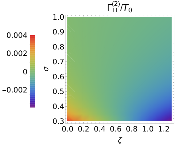
Even if a closed expression for the integral in Eq.(53) is not available, a numerical integration can be readily performed. On the left panel of Fig. 1 we show a density plot of the contribution $\Gamma^{(2)}_{TI}$ per unit time as a function of $\sigma$ and $\zeta$, while in the right panel we plot it as a function of $\sigma$ for several values of $\zeta$, setting in both cases the amplitude $\eta_{0}$ to one.

First of all, notice that $\Gamma^{(2)}_{TI}$ increases as $\sigma$ tends to zero, namely when the first term in the RHS of Eq.(49) prevails. This is to some extent hidden in the right panel of Fig. 1 for large values of $\zeta$, because the negative minimum also gets shifted towards smaller values of $\sigma$. Since in the small $\sigma$ limit the Gaußian becomes a delta function, the divergence is to be expected for two reasons: neither the interaction with a point delta potential in $D>2$ is well defined, nor the product $\eta^{2}$ which would involve two deltas.

Secondly, for fixed $\zeta$ and large $\sigma$, the value of $\Gamma^{(2)}_{TI}$ tends to zero. This is merely related to the normalization chosen for the Gaußian. Additionally, we observe that for fixed $\sigma$ the contribution changes sign as $\zeta$ increases, tending to a linear behavior. This agrees with the explicit expansion of $\Gamma^{(2)}_{TI}$ for small and large $\sigma\zeta$:

(54)

$\displaystyle\frac{\Gamma^{(2)}_{TI}}{T_{0}}=\begin{cases}\displaystyle\frac{1}{512\pi^{3}\sigma^{3}}\Big(\sqrt{\pi}+4\log(\sigma\zeta)\sigma\zeta+2(\gamma-\log(4))\sigma\zeta+\cdots\Big),\quad&\sigma\zeta\ll 1\\[8.5359pt] \displaystyle\frac{1}{\sigma^{3}}\left(-\frac{3\sigma\zeta}{256\pi^{3}}+\frac{1}{1152\pi^{3}\sigma\zeta}-\frac{1}{1200\pi^{3}\sigma^{3}\zeta^{3}}+\cdots\right),\quad&\sigma\zeta\gg 1\end{cases}.$

Nevertheless, this fact heavily depends on the chosen renormalization condition. As a way to clarify this assertion, consider the subtraction

(55)

$\displaystyle\begin{split}\frac{\Gamma^{(2)}_{m=0}}{T_{0}}:&=-\frac{\left|\eta_{0}\right|^{2}}{2({2\pi})^{2}}\int d\mathbf{k}^{\parallel}\,e^{-{\mathbf{k}^{\parallel}}^{2}\sigma^{2}}\left(F_{NL}(\mathbf{k}^{\parallel},\zeta)-\frac{3\zeta}{32\pi^{2}}\right),\end{split}$

which corresponds to a renormalization that will be called “null-mass” condition. Analogous to the previous case, we include in the left panel of Fig. 2 a density plot of $\Gamma^{(2)}_{m=0}$ per unit time as a function of $\zeta$ and $\sigma$, while the right panel corresponds to a plot as a function of $\sigma$ for different values of $\zeta$. From them it can be seen that, contrary to the precedent situation, the contribution to the effective action is strictly positive and shows no local minima. As emphasized before, this does not imply that the effective action has no physical meaning; it just points out the fact that one should formulate a theory describing the degrees of freedom encoded in $\eta$ and state a consistent renormalization prescription.

To show the plasticity of these formulas in Minkowski space, consider once more a Gaußian toy model,

(61)

$\displaystyle\eta_{G}({x}^{\parallel})=\eta_{0}\frac{e^{\frac{-(\mathbf{x}^{\parallel}-\mathbf{y}^{\parallel})^{2}}{2\sigma_{s}^{2}}}}{2\pi\sigma_{s}^{2}}\frac{e^{\frac{-(x^{0}-y^{0})^{2}}{2\sigma_{t}^{2}}}}{\sqrt{2\pi\sigma_{t}^{2}}},$

so that $\eta_{0}$ is a parameter of dimension length square in $D=4$ and, expliciting the Minkowskian metric, its Fourier transform reads

(62)

$\displaystyle\eta_{G}({k}^{\parallel})=\eta_{0}e^{-\frac{{\mathbf{k}^{\parallel}}^{2}\sigma_{s}^{2}}{2}-\frac{(k^{0})^{2}\sigma_{t}^{2}}{2}-i\mathbf{k}^{\parallel}\mathbf{y}^{\parallel}+ik^{0}y^{0}}.$

References

- [1] K.A. Milton “The Casimir effect: Physical manifestations of zero-point energy”, 2001 DOI: 10.1142/4505
- [2] M. Bordag, G.L. Klimchitskaya, U. Mohideen and V.M. Mostepanenko “Advances in the Casimir effect” Oxford University Press, 2009
- [3] Kimball. Milton “The Casimir effect: Recent controversies and progress” In J. Phys. A 37, 2004, pp. R209 DOI: 10.1088/0305-4470/37/38/R01
- [4] Kimball. Milton and Jef Wagner “Exact Casimir interaction between semitransparent spheres and cylinders” In Phys. Rev. D 77, 2008, pp. 045005 DOI: 10.1103/PhysRevD.77.045005
- [5] S.A.Franchino Vinas and P.A.G. Pisani “Semi-transparent Boundary Conditions in the Worldline Formalism” In J. Phys. A 44, 2011, pp. 295401 DOI: 10.1088/1751-8113/44/29/295401
- [6] Jose. Munoz-Castaneda, J. Mateos and A. Mosquera “Quantum vacuum energies and Casimir forces between partially transparent -function plates” In Phys. Rev. D 87.10, 2013, pp. 105020 DOI: 10.1103/PhysRevD.87.105020
- [7] V.V. Dodonov “Current status of the dynamical Casimir effect” In Phys. Scripta 82, 2010, pp. 038105 DOI: 10.1088/0031-8949/82/03/038105
- [8] Diego.R. Dalvit, Paulo. Maia and Francisco Mazzitelli “Fluctuations, dissipation and the dynamical Casimir effect” In Lect. Notes Phys. 834, 2011, pp. 419–457 DOI: 10.1007/978-3-642-20288-9˙13
- [9] P.D. Nation, J.R. Johansson, M.P. Blencowe and Franco Nori “Stimulating Uncertainty: Amplifying the Quantum Vacuum with Superconducting Circuits” In Rev. Mod. Phys. 84, 2012, pp. 1 DOI: 10.1103/RevModPhys.84.1
- [10] Valeri. Frolov and D. Singh “Quantum effects in the presence of expanding semitransparent spherical mirrors” In Class. Quant. Grav. 16, 1999, pp. 3693–3716 DOI: 10.1088/0264-9381/16/11/315
- [11] C.D. Fosco, F.C. Lombardo and F.D. Mazzitelli “Quantum dissipative effects in moving mirrors: A Functional approach” In Phys. Rev. D 76, 2007, pp. 085007 DOI: 10.1103/PhysRevD.76.085007
- [12] Jaume Haro and Emilio Elizalde “Black hole collapse simulated by vacuum fluctuations with a moving semitransparent mirror” In Phys. Rev. D 77, 2008, pp. 045011 DOI: 10.1103/PhysRevD.77.045011
- [13] Cesar. Fosco, Fernando. Lombardo and Francisco. Mazzitelli “Quantum dissipative effects in moving imperfect mirrors: sidewise and normal motions” In Phys. Rev. D 84, 2011, pp. 025011 DOI: 10.1103/PhysRevD.84.025011
- [14] C.D. Fosco, A. Giraldo and F.D. Mazzitelli “Dynamical Casimir effect for semitransparent mirrors” In Phys. Rev. D 96.4, 2017, pp. 045004 DOI: 10.1103/PhysRevD.96.045004
- [15] Martin Crocce, Diego.R. Dalvit, Fernando. Lombardo and Francisco. Mazzitelli “Resonant photon creation in a cavity with time dependent conductivity” In Phys. Rev. A 70, 2004, pp. 033811 DOI: 10.1103/PhysRevA.70.033811
- [16] Hector. Silva and C. Farina “A Simple model for the dynamical Casimir effect for a static mirror with time-dependent properties” In Phys. Rev. D 84, 2011, pp. 045003 DOI: 10.1103/PhysRevD.84.045003
- [17] Prachi Parashar, Kimball. Milton, K.V. Shajesh and Iver Brevik “Electromagnetic -function sphere” In Phys. Rev. D 96.8, 2017, pp. 085010 DOI: 10.1103/PhysRevD.96.085010
- [18] D. Deutsch and P. Candelas “Boundary Effects in Quantum Field Theory” In Phys. Rev. D 20, 1979, pp. 3063 DOI: 10.1103/PhysRevD.20.3063
- [19] Kimball. Milton “Local and Global Casimir Energies: Divergences, Renormalization, and the Coupling to Gravity” In Lect. Notes Phys. 834, 2011, pp. 39–95 DOI: 10.1007/978-3-642-20288-9˙3
- [20] Michael Bordag and D.V. Vassilevich “Nonsmooth backgrounds in quantum field theory” In Phys. Rev. D 70, 2004, pp. 045003 DOI: 10.1103/PhysRevD.70.045003
- [21] N. Graham et al. “Calculating vacuum energies in renormalizable quantum field theories: A New approach to the Casimir problem” In Nucl. Phys. B 645, 2002, pp. 49–84 DOI: 10.1016/S0550-3213(02)00823-4
- [22] Francisco. Mazzitelli, Jean Nery and Alejandro Satz “Boundary divergences in vacuum self-energies and quantum field theory in curved spacetime” In Phys. Rev. D 84, 2011, pp. 125008 DOI: 10.1103/PhysRevD.84.125008
- [23] Kimball. Milton “Hard and soft walls” In Phys. Rev. D 84, 2011, pp. 065028 DOI: 10.1103/PhysRevD.84.065028
- [24] Kimball. Milton et al. “Stress tensor for a scalar field in a spatially varying background potential” In Phys. Rev. D 93.8, 2016, pp. 085017 DOI: 10.1103/PhysRevD.93.085017
- [25] Michael Bordag, K. Kirsten and D. Vassilevich “On the ground state energy for a penetrable sphere and for a dielectric ball” In Phys. Rev. D 59, 1999, pp. 085011 DOI: 10.1103/PhysRevD.59.085011
- [26] Michael Bordag, Meik Hellmund and Klaus Kirsten “Dependence of the vacuum energy on spherically symmetric background fields” In Phys. Rev. D 61, 2000, pp. 085008 DOI: 10.1103/PhysRevD.61.085008
- [27] Klaus Kirsten “Spectral functions in mathematics and physics”, 2001
- [28] Cesar. Fosco and Francisco. Mazzitelli “Casimir energy due to inhomogeneous thin plates” In Phys. Rev. D 101.4, 2020, pp. 045012 DOI: 10.1103/PhysRevD.101.045012
- [29] Christian Schubert “Perturbative quantum field theory in the string inspired formalism” In Phys. Rept. 355, 2001, pp. 73–234 DOI: 10.1016/S0370-1573(01)00013-8
- [30] D. Bauch “The path integral for a particle moving in a -function potential” In Il Nuovo Cimento B (1971-1996) 85, 1985, pp. 118–124 DOI: 10.1007/BF02721525
- [31] B Gaveau and L Schulman “Explicit time-dependent Schrodinger propagators” In Journal of Physics A: Mathematical and General 19.10 IOP Publishing, 1986, pp. 1833–1846 DOI: 10.1088/0305-4470/19/10/024
- [32] James. Edwards and Christian Schubert “Quantum mechanical path integrals in the first quantised approach to quantum field theory”, 2019 arXiv:1912.10004 [hep-th]
- [33] José Nicasio, Naser Ahmadiniaz, James. Edwards and Christian Schubert “Non-perturbative gauge transformations of arbitrary fermion correlation functions in quantum electrodynamics”, 2020 arXiv:2010.04160 [hep-th]
- [34] S.A. Franchino-Viñas and S. Mignemi “Worldline Formalism in Snyder Spaces” In Phys. Rev. D 98.6, 2018, pp. 065010 DOI: 10.1103/PhysRevD.98.065010
- [35] Michael Bordag and D.V. Vassilevich “Heat kernel expansion for semitransparent boundaries” In J. Phys. A 32, 1999, pp. 8247–8259 DOI: 10.1088/0305-4470/32/47/304
- [36] D.V. Vassilevich “Heat kernel expansion: User’s manual” In Phys. Rept. 388, 2003, pp. 279–360 DOI: 10.1016/j.physrep.2003.09.002
- [37] A.O. Barvinsky and G.A. Vilkovisky “Beyond the Schwinger-Dewitt Technique: Converting Loops Into Trees and In-In Currents” In Nucl. Phys. B 282, 1987, pp. 163–188 DOI: 10.1016/0550-3213(87)90681-X
- [38] I.G. Avramidi “The Covariant Technique for Calculation of One Loop Effective Action” [Erratum: Nucl.Phys.B 509, 557–558 (1998)] In Nucl. Phys. B 355, 1991, pp. 712–754 DOI: 10.1016/0550-3213(91)90492-G
- [39] A.O. Barvinsky and G.A. Vilkovisky “The Generalized Schwinger-Dewitt Technique in Gauge Theories and Quantum Gravity” In Phys. Rept. 119, 1985, pp. 1–74 DOI: 10.1016/0370-1573(85)90148-6
- [40] C.G. Beneventano and E.M. Santangelo “Connection between zeta and cutoff regularizations of Casimir energies” In Int. J. Mod. Phys. A 11, 1996, pp. 2871–2886 DOI: 10.1142/S0217751X96001395
- [41] Cesar. Fosco, Fernando. Lombardo and Francisco. Mazzitelli “Derivative expansion for the Casimir effect at zero and finite temperature in dimensions” In Phys. Rev. D 86, 2012, pp. 045021 DOI: 10.1103/PhysRevD.86.045021
- [42] P.A. Maia, A. Lambrecht and S. Reynaud “Roughness correction to the Casimir force: Beyond the proximity force approximation” [Erratum: EPL 100, 29902 (2012)] In Europhys. Lett. 69.9, 2005, pp. 924 DOI: 10.1209/0295-5075/100/29902
- [43] C. Itzykson and J.. Zuber “Quantum Field Theory” New York: McGraw-Hill Inc., 1980
- [44] Joshua. Frieman “Particle Creation in Inhomogeneous Space-times” In Phys. Rev. D 39, 1989, pp. 389 DOI: 10.1103/PhysRevD.39.389
- [45] Sebastián Franchino-Viñas and Holger Gies “Propagator from Nonperturbative Worldline Dynamics” In Phys. Rev. D 100.10, 2019, pp. 105020 DOI: 10.1103/PhysRevD.100.105020