跳到论文正文
W Papers独立论文阅读器 arXiv:2010.10844 论文正文 计算阅读时间 · 0%
引用这篇论文根据当前论文元数据生成,正式投稿前建议核对。


License: arXiv.org perpetual non-exclusive license
arXiv:2010.10844v2 [cs.CE] 25 May 2021

Topology optimization of acoustic metasurfaces by using a two-scale homogenization method Journal: Elsevier

Yuki Noguchi Email: noguchi@mech.t.u-tokyo.ac.jp Corresponding author: Corresponding author. Tel.: +81-3-5841-0294; Fax: +81-3-5841-0294.    Takayuki Yamada Address: Department of Strategic Studies, Institute of Engineering Innovation, School of Engineering, The University of Tokyo, Yayoi 2-11-16, Bunkyo–ku, Tokyo 113-8656, Japan.
Abstract

In this paper, we propose a level set-based topology optimization method for the unit-cell design of acoustic metasurfaces by using a two-scale homogenization method. Based on previous works, we first propose a homogenization method for acoustic metasurfaces that can be combined with topology optimization. In this method, a nonlocal transmission condition depending on the unit cell of the metasurface appears in a macroscale problem. Next, we formulate an optimization problem within the framework of a level set-based topology optimization method, wherein an objective functional is expressed as the macroscopic responses obtained through the homogenization, and material distributions in the unit cell are set as design variables. A sensitivity analysis is conducted based on the concept of the topological derivative. To confirm the validity of the proposed method, two-dimensional numerical examples are provided. First, we provide a numerical example that supports the validity of the homogenization method, and we then perform optimization calculations based on the waveguide settings of the acoustic metasurfaces. In addition, we discuss the mechanism of the obtained optimized structures.

Keywords: 
Acoustic metasurface , Two-scale homogenization method , Topology optimization , Level set method , Acoustic metamaterial , Topological derivative

1 Introduction

Acoustic metamaterials are artificial composite materials that exhibit unusual acoustic performance that cannot be achieved by naturally existing acoustic media. The concept of acoustic metamaterials is derived from that of the metamaterials of electromagnetic waves, which was first proposed by Veselago [1]. Several researchers have reported on electromagnetic metamaterials and their many unusual properties, represented by a negative refractive index. The first extension of the concept of metamaterials to acoustic waves was a locally resonant sonic material proposed by Liu et al. [2]. It is composed of a periodic array of unit cells filled with various elastic media, and the local resonance phenomenon is induced in the unit cell, producing a bandgap that prevents the transmission of acoustic waves. After this pioneering work, various studies have proposed acoustic metamaterials exhibiting various characteristics, such as negative bulk modulus [3], negative mass density [4, 5], and negative refractive index [6, 7]. These unusual acoustic properties can be used for the efficient control of acoustic waves and development of novel acoustic devices, such as an acoustic cloaking device [8] and acoustic hyperlens [9].

Although typical acoustic metamaterials have three-dimensional arrays of unit cells, current research interests are focused on the planar type of acoustic metamaterials, called acoustic metasurfaces. Acoustic metasurfaces are based on the two-dimensional array of unit cells with finite thickness; they efficiently control acoustic waves in a smaller region compared to the bulk acoustic metamaterials. Various types of metasurfaces that exhibit unusual acoustic properties have been proposed, for example, the sound-absorbing metasurface using the resonance of membrane structure [10], a metasurface that manipulates the wavefront of acoustic waves by shifting their phase by using the complex structure of the unit cells [11].

These extraordinary properties of metasurfaces strongly depend on their unit-cell structure. Therefore, the structural design of a unit cell is essential to obtain the desired acoustic behaviors. As metasurfaces control acoustic waves in a narrow region compared to bulk metamaterials, efficient structural design is required. Hence, we introduce a topology optimization method, with the highest degree of design freedom among structural optimization methods. Since the introduction of the method for linear elasticity problems [12], it has been applied in a wide range of fields including wave-propagation problems [13]. Regarding the applications of topology optimization to acoustic-wave-propagation problems, Wadbro and Berggren [14] proposed a topology optimization method for the design of an acoustic horn that transmits acoustic waves efficiently. Du and Olhoff [15] optimized a bi-material structure to minimize sound radiation from the surface. Dühring et al. [16] proposed the SIMP method for acoustic problems to reduce indoor and outdoor noises. Furthermore, acoustic-structural interaction problems can be considered in topology optimization, as suggested by [17].

Topology optimization has also been applied for the design of metamaterials and metasurfaces. Diaz and Sigmund [18] proposed a topology optimization method for electromagnetic metamaterials and showed that the obtained designs of the unit cell exhibited a negative permeability. Lu et al.[19] pointed out that acoustic metamaterials are optimized based on a level set-based topology optimization method and exhibit a negative bulk modulus. The optimum design of an acoustic metasurface that converts longitudinal elastic waves into transverse elastic waves was derived in [20]. Christiansen and Sigmund [21] conducted topology optimization for a finite acoustic metamaterial slab, and they obtained its unit cell design inducing negative refraction. Roca et al. [22] combined a multiscale homogenization approach based on a generalized Hill-Mandel principle with topology optimization; they obtained the unit cell design of locally resonant acoustic metamaterials.

When determining the optimum design of acoustic metasurfaces using the topology optimization method, the computational cost must be considered because the optimization procedure comprises iterative analyses of the metasurface system, which is defined as the aggregation of unit cells with complex geometries. The S-parameters-based retrieval method proposed by Smith et al. [23] is used to obtain the macroscopic properties of metamaterials and metasurfaces, and it was first applied to electromagnetic metamaterials; its application was later expanded to acoustic metamaterials [24]. Once the S-parameters representing the complex transmission and reflection coefficients are obtained, the effective material parameters of the metamaterials, such as the effective refractive index, can be estimated. Although this method is simple and easy to implement, its application to general systems of a metasurface with complex incident-wave conditions is difficult, as it is based on the assumption that waves can be expressed as plane waves.

Homogenization is another method used to estimate the macroscopic properties of metasurfaces. The classical homogenization method [25, 26, 27] is based on the asymptotic expansion of the solution using two types of characteristic scales: microscale and macroscale. By adopting this method for a system composed of a periodic array of unit cells, its complex structure is equivalently replaced with a homogeneous material, the properties of which are expressed through homogenized coefficients. This method holds for static or quasi-static problems, in which the wavelength of the waves traveling within the periodic structure is significantly longer than the size of the unit cell. To address the problems involved with shorter wavelengths, where the quasi-static limit cannot be applied, a higher-order homogenization method [28, 29, 30, 31, 32] was proposed. This is an extended version of the homogenization method and considers higher order terms, based on which the method allows for the modeling of the size effects of unit cells. For a wavelength that is considerably shorter but has a similar order as the unit cell, a high-frequency homogenization method [33] was proposed based on asymptotic expansions of the solution and frequency. This method analyzes the perturbations of standing waves induced in the unit cell and can be applied to estimate the performance of metamaterials or photonic crystals [34]. Furthermore, topology optimization was combined with this method for designing hyperbolic acoustic metamaterials [35].

These homogenization methods target perfectly periodic infinite media composed of an array of unit cells, such as a square lattice in a two-dimensional problem. As the metasurface has a finite thickness, special treatments are required in the homogenization method for dealing with such a metasurface. Marigo and Maurel [36, 37] proposed a homogenization method for metasurfaces in which higher-order approximation was introduced with inner and outer asymptotic expansions, which correspond to the region near the unit cells and the surrounding medium of the periodic array of unit cells, respectively. Rohan and Lukeš [38] proposed a homogenization method for thin structures, the thickness of which was assumed to have the same order as the period of the unit cells. In [38], the system of a rigid plate with periodic perforations was decomposed into a fictitious layer containing rigid obstacles and other regions filled with the background acoustic medium. The two-scale homogenization limit resulted in a homogeneous acoustic system with a nonlocal transmission condition imposed on the interface, which is a limited form of the fictitious layer. This method was later extended to consider the oscillation of the elastic plate comprising the metasurface by introducing the Reissner–Mindlin plate model [39]. In the context of optimization, a shape sensitivity analysis was also conducted [40, 41] to be used in the shape optimization of the metasurface; however, no study has reported on topology optimization thus far.

In this research, we developed a topology optimization method for designing acoustic metasurfaces based on the homogenization method proposed by Rohan and Lukeš. Based on the proposed method, the material distribution in a single unit cell of the metasurface is optimized such that the metasurface composed of the optimized unit cells exhibits the desired macroscopic performance. The remainder of this paper is organized as follows. Section 2 introduces the homogenization method for acoustic metasurfaces. We extend the previous method [38] for rigid obstacles to the system composed of two media, in which waves are described by the Helmholtz equation, to ensure that topology optimization can be introduced. Next, in section 3, the design problem for acoustic metasurfaces is formulated based on the two-dimensional settings. In section 4, we explain the topology optimization for acoustic metasurfaces. The setting of the objective functional is provided within the framework of the homogenization method, and sensitivity analysis is conducted based on the concept of the topological derivative. Then, section 5 briefly explains the proposed level set-based topology optimization. The numerical implementation is described in section 6, which also presents the optimization process and discretization method using the finite element model (FEM) for the governing and adjoint equations. In section 7, several two-dimensional numerical examples are provided. Here, an example that supports the validity of the proposed homogenization method is first provided, and then the optimization results of waveguiding acoustic metasurfaces are presented. To confirm the obtained results, we conducted acoustic-wave-propagation analysis based on the FEM for the entire system of the metasurfaces without using the homogenization method. Finally, we provide the conclusions drawn from this study in section 8.

2 Homogenization method for acoustic metasurfaces

Refer to caption
Figure 1: Geometrical settings: (a) Original system of an acoustic metasurface. (b) The homogenized system of (a) with macroscale and microscale problems.

In this section, we introduce a homogenization method for acoustic metasurfaces based on a previous method [38, 39]. Figure 1(a) presents the system of an acoustic metasurface. Cartesian coordinate 𝒙=(𝒙′,xd)\bm{x}=(\bm{x}^{\prime},x_{d}) is used, and it comprises 𝒙′∈𝐑N−1\bm{x}^{\prime}\in\mathbf{R}^{N-1} and xd∈𝐑x_{d}\in\mathbf{R}, where N=2N=2 or 33 represents the spatial dimension. Unit cells with period ϵ\epsilon of the metasurface are periodically arranged along 𝒙′\bm{x}^{\prime}, and they have a finite thickness of δ\delta along xdx_{d}. For the homogenization procedure, thickness δ\delta is assumed to be of the similar order as ϵ\epsilon. Then, δ\delta can be expressed as δ=κ​ϵ\delta=\kappa\epsilon with κ>0\kappa>0. The array of unit cells forms a rectangular domain of Ωϵ\Omega^{\epsilon}, called as a transmission layer. It is connected with the two outer regions of Ω±\Omega^{\pm}, where incident, reflected, and transmitted waves can propagate. Γ±\Gamma^{\pm} represents the interfaces between Ωϵ\Omega^{\epsilon} and Ω±\Omega^{\pm}, whereas Γ0\Gamma^{0} represents the mid-plane of Ωϵ\Omega^{\epsilon}. We set the origin of coordinate 𝒙=(𝒙′,xd)\bm{x}=(\bm{x^{\prime}},x_{d}) such that Γ0\Gamma^{0} can be expressed as Γ0={𝒙∈ΩG|xd=0}\Gamma^{0}=\{\bm{x}\in\Omega^{G}|~x_{d}=0\}, where ΩG=Ω+∪Ω−∪Ωϵ\Omega^{G}=\Omega^{+}\cup\Omega^{-}\cup\Omega^{\epsilon} represents the entire domain. Then, interfaces Γ±\Gamma^{\pm} are expressed as Γ±={𝒙∈ΩG|xd=∓δ2}\Gamma^{\pm}=\{\bm{x}\in\Omega^{G}|~x_{d}=\mp\frac{\delta}{2}\}.

By assuming a harmonic oscillation with angular frequency ω\omega, the boundary value problem corresponding to the system shown in Fig. 1(a) is described as follows:

∇⋅(1ρ⁡(𝒙)∇p)+ω2K⁡(𝒙)p\displaystyle\nabla\cdot\left(\frac{1}{\rho(\bm{x})}\nabla p\right)+\frac{\omega^{2}}{K(\bm{x})}p =0​in​ΩG,\displaystyle=0~~\mathrm{in~}\Omega^{G}, (1)
𝒏⋅(1ρ0∇p)+i​k0ρ0p\displaystyle\bm{n}\cdot\left(\frac{1}{\rho_{0}}\nabla p\right)+\frac{ik_{0}}{\rho_{0}}p =2​i​k0ρ0​Pin​on​Γin,\displaystyle=\frac{2ik_{0}}{\rho_{0}}P_{\mathrm{in}}~~\mathrm{on~}\Gamma_{\mathrm{in}}, (2)
𝒏⋅(1ρ0∇p)+i​k0ρ0p\displaystyle\bm{n}\cdot\left(\frac{1}{\rho_{0}}\nabla p\right)+\frac{ik_{0}}{\rho_{0}}p =0​on​Γout,\displaystyle=0~~\mathrm{on~}\Gamma_{\mathrm{out}}, (3)
𝒏⋅(1ρ⁡(𝒙)∇p)\displaystyle\bm{n}\cdot\left(\frac{1}{\rho(\bm{x})}\nabla p\right) =0​on​∂extΩG∖(Γin∪Γout),\displaystyle=0~~\mathrm{on~}\partial_{\mathrm{ext}}{\Omega^{G}}\setminus(\Gamma_{\mathrm{in}}\cup\Gamma_{\mathrm{out}}), (4)

where pp represents the complex amplitude of acoustic pressure, and ∂extΩG\partial_{\mathrm{ext}}\Omega^{G} represents the external boundary of the entire domain, ΩG\Omega^{G}. The mass density ρ\rho and bulk modulus KK have piece-wise constant distributions in Ωϵ\Omega^{\epsilon} corresponding to the structural configuration of the metasurface, whereas they are constant in Ω±\Omega^{\pm}, denoted by ρ0\rho_{0} and K0K_{0} respectively. Eq. (2) represents an incident-wave boundary condition on Γin\Gamma_{\mathrm{in}}, the amplitude and wavenumber of which are PinP_{\mathrm{in}} and k0k_{0}, respectively. Eq. (3) represents an absorbing boundary condition on Γout\Gamma_{\mathrm{out}} to reduce the reflected waves, and sound-hard conditions are applied to the other external boundaries.

By introducing the homogenization method, we aim to replace the complex structure of the metasurface in Ωϵ\Omega^{\epsilon} with an equivalent interface, Γ0\Gamma^{0}, by considering the limit ϵ→0\epsilon\to 0, on which there can be jumps in acoustic pressure and flux. When ϵ→0\epsilon\to 0, boundaries Γ±\Gamma^{\pm} approach Γ0\Gamma^{0} and transmission layer Ωϵ\Omega^{\epsilon} degenerates to Γ0\Gamma^{0}.

As the metasurface has a finite thickness, the original boundary value problem must first be decomposed into the problems defined in the transmission layer Ωϵ\Omega^{\epsilon} and outer regions Ω±\Omega^{\pm}. Given the acoustic pressure on Γ±\Gamma^{\pm} expressed by pgϵp_{g}^{\epsilon}, the boundary value problem for Ω±\Omega^{\pm} is summarized as follows:

1ρ0​∇2P±+ω2K0​P±\displaystyle\frac{1}{\rho_{0}}\nabla^{2}P^{\pm}+\frac{\omega^{2}}{K_{0}}P^{\pm} =0​in​Ω+∪Ω−\displaystyle=0~~\mathrm{in~}\Omega^{+}\cup\Omega^{-} (5)
P±\displaystyle P^{\pm} =pgϵ​on​Γ±\displaystyle=p_{g}^{\epsilon}~~\mathrm{on~}\Gamma^{\pm} (6)
𝒏⋅(1ρ0∇P)+i​k0ρ0P\displaystyle\bm{n}\cdot\left(\frac{1}{\rho_{0}}\nabla P\right)+\frac{ik_{0}}{\rho_{0}}P =0​on​Γout,\displaystyle=0~~\mathrm{on~}\Gamma_{\mathrm{out}}, (7)
𝒏⋅(1ρ0∇P)+i​k0ρ0P\displaystyle\bm{n}\cdot\left(\frac{1}{\rho_{0}}\nabla P\right)+\frac{ik_{0}}{\rho_{0}}P =2​i​k0ρ0​Pin​on​Γin,\displaystyle=\frac{2ik_{0}}{\rho_{0}}P_{\mathrm{in}}~~\mathrm{on~}\Gamma_{\mathrm{in}}, (8)
𝒏⋅(1ρ0∇P)\displaystyle\bm{n}\cdot\left(\frac{1}{\rho_{0}}\nabla P\right) =0​on​∂extΩ±∖(Γin∪Γout),\displaystyle=0~~\mathrm{on~}\partial_{\mathrm{ext}}\Omega^{\pm}\setminus(\Gamma_{\mathrm{in}}\cup\Gamma_{\mathrm{out}}), (9)

Similarly, given the fluxes on Γ±\Gamma^{\pm} expressed by gϵ±g^{\epsilon\pm}, the boundary value problem for transmission layer Ωϵ\Omega^{\epsilon} to determine the unknown pϵp^{\epsilon} is summarized as follows:

∇⋅(1ρ⁡(𝒙)∇pϵ)+ω2K⁡(𝒙)pϵ\displaystyle\nabla\cdot\left(\frac{1}{\rho(\bm{x})}\nabla p^{\epsilon}\right)+\frac{\omega^{2}}{K(\bm{x})}p^{\epsilon} =0​in​Ωϵ,\displaystyle=0~~\mathrm{in~}\Omega^{\epsilon}, (10)
𝒏⋅(1ρ0∇pϵ)\displaystyle\bm{n}\cdot\left(\frac{1}{\rho_{0}}\nabla p^{\epsilon}\right) =−gϵ±​on​Γ±,\displaystyle=-g^{\epsilon\pm}~~\mathrm{on~}\Gamma^{\pm}, (11)
𝒏⋅(1ρ0∇pϵ)\displaystyle\bm{n}\cdot\left(\frac{1}{\rho_{0}}\nabla p^{\epsilon}\right) =0​on​∂Ωϵ∖Γ±.\displaystyle=0~~\mathrm{on~}\partial\Omega^{\epsilon}\setminus\Gamma^{\pm}. (12)

The abovementioned decoupled problems are equivalent to the original boundary value problem if the following coupling conditions on Γ±\Gamma^{\pm} hold:

pϵ\displaystyle p^{\epsilon} =pgϵ=P±​on​Γ±,\displaystyle=p_{g}^{\epsilon}=P^{\pm}~~~\mathrm{on~}\Gamma^{\pm}, (13)
gϵ±\displaystyle g^{\epsilon\pm} =𝒏±⋅(1ρ0∇P±)onΓ±.\displaystyle=\bm{n}^{\pm}\cdot\left(\frac{1}{\rho_{0}}\nabla P^{\pm}\right)~~\mathrm{on~}\Gamma^{\pm}. (14)

Next, we establish a homogenized system for transmission layer Ωϵ\Omega^{\epsilon}. First, the weak form of the system in Ωϵ\Omega^{\epsilon} is expressed as follows:

∫Ωϵ1ρ⁡(𝒙)∇pϵ⋅∇qϵdΩ−∫Ωϵω2K⁡(𝒙)pϵqϵdΩ=−∫Γ±gϵ±qϵdΓ∀qϵ∈H1(Ωϵ).\displaystyle\int_{\Omega^{\epsilon}}\frac{1}{\rho(\bm{x})}\nabla p^{\epsilon}\cdot\nabla q^{\epsilon}d\Omega-\int_{\Omega^{\epsilon}}\frac{\omega^{2}}{K(\bm{x})}p^{\epsilon}q^{\epsilon}d\Omega=-\int_{\Gamma^{\pm}}g^{\epsilon\pm}q^{\epsilon}d\Gamma~~~\forall q^{\epsilon}\in H^{1}(\Omega^{\epsilon}). (15)

We introduce the scaled coordinate in the direction of xdx_{d} as z=1ϵ​xdz=\frac{1}{\epsilon}x_{d}. Then, transmission layer Ωϵ\Omega^{\epsilon} can be expressed as Ω^=Γ0×]−κ2,κ2[\hat{\Omega}=\Gamma^{0}\times]-\frac{\kappa}{2},\frac{\kappa}{2}[ by using scaled coordinate (𝒙′,z)(\bm{x^{\prime}},z). For this coordinate, equation (15) is modified as

∫Ω^1ρ⁡(𝒙)(∇¯pϵ⋅∇¯qϵ+1ϵ2∂pϵ∂z∂qϵ∂z)dΩ−∫Ω^ω2K⁡(𝒙)pϵqϵdΩ=−1ϵ∫Γ±gϵ±qϵdΓ,\displaystyle\int_{\hat{\Omega}}\frac{1}{\rho(\bm{x})}\left(\overline{\nabla}p^{\epsilon}\cdot\overline{\nabla}q^{\epsilon}+\frac{1}{\epsilon^{2}}\frac{\partial p^{\epsilon}}{\partial z}\frac{\partial q^{\epsilon}}{\partial z}\right)d\Omega-\int_{\hat{\Omega}}\frac{\omega^{2}}{K(\bm{x})}p^{\epsilon}q^{\epsilon}d\Omega=-\frac{1}{\epsilon}\int_{\Gamma^{\pm}}g^{\epsilon\pm}q^{\epsilon}d\Gamma, (16)

where ∇¯\overline{\nabla} is an in-plane gradient, the components of which are denoted by ∂∂xα​(α=1,…,N−1)\frac{\partial}{\partial x_{\alpha}}~(\alpha=1,...,N-1).

In previous studies [38, 39], the periodic unfolding method was used to homogenize the system with the unfolding operator TϵT_{\epsilon}. The operator TϵT_{\epsilon} associates solution v∈Lp​(Ω)v\in L^{p}(\Omega) with Tϵ​(v)∈Lp​(Ω×Y)T_{\epsilon}(v)\in L^{p}(\Omega\times Y), where domain Ω\Omega contains a periodic structure characterized by the representative unit cell, YY. One of the important properties of TϵT_{\epsilon} is the so-called integral conservation, which is represented as follows:

∫Ωv⁡(𝒙)​d​Ωx=1|Y|​∫Ω×YTϵ​(v)​(𝒙,𝒚)​d​Ωx​d​Ωy.\displaystyle\int_{\Omega}v(\bm{x})d\Omega_{x}=\frac{1}{|Y|}\int_{\Omega\times Y}T_{\epsilon}(v)(\bm{x},\bm{y})d\Omega_{x}d\Omega_{y}. (17)

Details regarding the periodic unfolding method and the properties of TϵT_{\epsilon} can be referenced from [42].

To introduce the periodic unfolding method into the system of the metasurface, a scaled coordinate is defined in the direction of 𝒙′\bm{x^{\prime}} as 𝒚′=𝒙′ϵ\bm{y^{\prime}}=\frac{\bm{x^{\prime}}}{\epsilon}. The microscale coordinate 𝒚=(𝒚′,z)\bm{y}=(\bm{y^{\prime}},z) is utilized to express the representative unit cell, YY, as shown in Fig. 1(b). Thereafter, the unfolding operator TϵT_{\epsilon} is defined such that it maps solution pϵ∈L2​(Ωϵ)p^{\epsilon}\in L^{2}(\Omega^{\epsilon}) to Tϵ​(pϵ)∈L2​(Γ0×Y)T_{\epsilon}(p^{\epsilon})\in L^{2}(\Gamma^{0}\times Y).

We impose the following assumption on fluxes gϵ±g^{\epsilon\pm}:

gϵ+​(𝒙′)=g0​(𝒙′)+ϵ​g1+​(𝒙′,𝒙′ϵ),\displaystyle g^{\epsilon+}(\bm{x^{\prime}})=g^{0}(\bm{x^{\prime}})+\epsilon g^{1+}(\bm{x^{\prime}},\frac{\bm{x^{\prime}}}{\epsilon}), (18)
gϵ−​(𝒙′)=−g0​(𝒙′)−ϵ​g1−​(𝒙′,𝒙′ϵ),\displaystyle g^{\epsilon-}(\bm{x^{\prime}})=-g^{0}(\bm{x^{\prime}})-\epsilon g^{1-}(\bm{x^{\prime}},\frac{\bm{x^{\prime}}}{\epsilon}), (19)

These assumptions assure the continuity of the lowest order of fluxes across Γ±\Gamma^{\pm} and are expressed as g0​(𝒙′)g^{0}(\bm{x^{\prime}}). The opposite signs in the definition of gϵ±g^{\epsilon\pm} are due to the outward normal vector on Γ±\Gamma^{\pm}. Under this assumption and the weak form in Eq. (16), a priori estimates to the solution (see [38, 39]) lead to the following convergence results for ϵ→0\epsilon\to 0:

Tϵ​(pϵ)⇀p0\displaystyle T_{\epsilon}(p^{\epsilon})\rightharpoonup p^{0}~~~ weakly​in​L2​(Γ0×Y),\displaystyle\mathrm{weakly~in~}L^{2}(\Gamma_{0}\times Y), (20)
Tϵ​(∇¯​pϵ)⇀∇¯x​p0+∇¯y​p1\displaystyle T_{\epsilon}(\overline{\nabla}p^{\epsilon})\rightharpoonup\overline{\nabla}_{x}p^{0}+\overline{\nabla}_{y}p^{1}~~~ weakly​in​L2​(Γ0×Y),\displaystyle\mathrm{weakly~in~}L^{2}(\Gamma_{0}\times Y), (21)
1ϵ​Tϵ​(∂pϵ∂z)⇀∂p1∂z\displaystyle\frac{1}{\epsilon}T_{\epsilon}(\frac{\partial p^{\epsilon}}{\partial z})\rightharpoonup\frac{\partial p^{1}}{\partial z}~~~ weakly​in​L2​(Γ0×Y),\displaystyle\mathrm{weakly~in~}L^{2}(\Gamma_{0}\times Y), (22)

where ∇¯x\overline{\nabla}_{x} and ∇¯y\overline{\nabla}_{y} denote in-plane gradients with respect to 𝒙′∈Γ0\bm{x^{\prime}}\in\Gamma_{0} and 𝒚′∈Y\bm{y^{\prime}}\in Y, respectively. p0∈H1​(Γ0)p^{0}\in H^{1}(\Gamma^{0}) and p1∈L2​(Γ0,H♯¯1)p^{1}\in L^{2}(\Gamma^{0};H^{1}_{\underline{\sharp}}) are asymptotic expanded pressures, where H♯¯1​(Y)H^{1}_{\underline{\sharp}}(Y) represents a subspace of H1​(Y)H^{1}(Y) that satisfies the periodic boundary conditions in the direction of yα(α=1,..,N−1)y_{\alpha}~(\alpha=1,..,N-1).

By using these results, the following homogenized equation is obtained:

∑α=1N−1∑β=1N−1∫Γ0Aα​β∗∂p0∂xβ∂q0∂xαdΓx−ω2∫Γ0K−1∗p0q0dΓx+∫Γ0g0𝑩∗⋅∇¯xq0dΓx\displaystyle\sum_{\alpha=1}^{N-1}\sum_{\beta=1}^{N-1}\int_{\Gamma^{0}}A_{\alpha\beta}^{\ast}\frac{\partial p^{0}}{\partial x_{\beta}}\frac{\partial q^{0}}{\partial x_{\alpha}}d\Gamma_{x}-\omega^{2}\int_{\Gamma^{0}}K^{-1\ast}p^{0}q^{0}d\Gamma_{x}+\int_{\Gamma^{0}}g^{0}\bm{B}^{\ast}\cdot\overline{\nabla}_{x}q^{0}d\Gamma_{x}
=−∫Γ0q0(−∫ΘΔg1dΓy)dΓx,\displaystyle=-\int_{\Gamma^{0}}q^{0}\left(\mathchoice{{\vbox{\hbox{$\textstyle-$ }}\kern-7.83337pt}}{{\vbox{\hbox{$\scriptstyle-$ }}\kern-6.11674pt}}{{\vbox{\hbox{$\scriptscriptstyle-$ }}\kern-5.48965pt}}{{\vbox{\hbox{$\scriptscriptstyle-$ }}\kern-5.31259pt}}\!\int_{\Theta}\Delta g^{1}d\Gamma_{y}\right)d\Gamma_{x}, (23)

where Δ​g1\Delta g^{1} is used to express the difference between g1±g^{1\pm} as Δ​g1=g1+−g1−\Delta g^{1}=g^{1+}-g^{1-}. Aα​β∗A_{\alpha\beta}^{\ast}, 𝑩∗\bm{B}^{\ast}, and K−1∗K^{-1\ast} are homogenized coefficients, and they are expressed as

Aα​β∗=−∫Y1ρ⁡(𝒚){∇¯y(ηβ+yβ)⋅∇¯y(ηα+yα)+∂ηβ∂z∂ηα∂z}dΩy,\displaystyle A_{\alpha\beta}^{\ast}=\mathchoice{{\vbox{\hbox{$\textstyle-$ }}\kern-7.83337pt}}{{\vbox{\hbox{$\scriptstyle-$ }}\kern-6.11674pt}}{{\vbox{\hbox{$\scriptscriptstyle-$ }}\kern-5.48965pt}}{{\vbox{\hbox{$\scriptscriptstyle-$ }}\kern-5.31259pt}}\!\int_{Y}\frac{1}{\rho(\bm{y})}\left\{\overline{\nabla}_{y}({\color[rgb]{0,0,0}\eta}^{\beta}+y_{\beta})\cdot\overline{\nabla}_{y}({\color[rgb]{0,0,0}\eta}^{\alpha}+y_{\alpha})+\frac{\partial{\color[rgb]{0,0,0}\eta}^{\beta}}{\partial z}\frac{\partial{\color[rgb]{0,0,0}\eta}^{\alpha}}{\partial z}\right\}d\Omega_{y}, (24)
𝑩∗=−∫Y1ρ⁡(𝒚)∇¯yξdΩy,\displaystyle\bm{B}^{\ast}=\mathchoice{{\vbox{\hbox{$\textstyle-$ }}\kern-7.83337pt}}{{\vbox{\hbox{$\scriptstyle-$ }}\kern-6.11674pt}}{{\vbox{\hbox{$\scriptscriptstyle-$ }}\kern-5.48965pt}}{{\vbox{\hbox{$\scriptscriptstyle-$ }}\kern-5.31259pt}}\!\int_{Y}\frac{1}{\rho(\bm{y})}\overline{\nabla}_{y}\xi d\Omega_{y}, (25)
K−1∗=−∫Y1K⁡(𝒚)dΩy.\displaystyle K^{-1\ast}=\mathchoice{{\vbox{\hbox{$\textstyle-$ }}\kern-7.83337pt}}{{\vbox{\hbox{$\scriptstyle-$ }}\kern-6.11674pt}}{{\vbox{\hbox{$\scriptscriptstyle-$ }}\kern-5.48965pt}}{{\vbox{\hbox{$\scriptscriptstyle-$ }}\kern-5.31259pt}}\!\int_{Y}\frac{1}{K(\bm{y})}d\Omega_{y}. (26)

To estimate these homogenized coefficients, functions, ηα{\color[rgb]{0,0,0}\eta}^{\alpha} and ξ\xi, defined in the microscale 𝒚\bm{y}, are introduced. They are the solutions of the following cell problems:

−∫Y1ρ⁡(𝒚)(∇¯yηα⋅∇¯yψ+∂ηα∂z∂ψ∂z)dΩy=−−∫Y1ρ⁡(𝒚)∂ψ∂yαdΩy∀ψ∈H♯¯1(Y),\displaystyle\mathchoice{{\vbox{\hbox{$\textstyle-$ }}\kern-7.83337pt}}{{\vbox{\hbox{$\scriptstyle-$ }}\kern-6.11674pt}}{{\vbox{\hbox{$\scriptscriptstyle-$ }}\kern-5.48965pt}}{{\vbox{\hbox{$\scriptscriptstyle-$ }}\kern-5.31259pt}}\!\int_{Y}\frac{1}{\rho(\bm{y})}\left(\overline{\nabla}_{y}{\color[rgb]{0,0,0}\eta}^{\alpha}\cdot\overline{\nabla}_{y}\psi+\frac{\partial{\color[rgb]{0,0,0}\eta}^{\alpha}}{\partial z}\frac{\partial\psi}{\partial z}\right)d\Omega_{y}=-\mathchoice{{\vbox{\hbox{$\textstyle-$ }}\kern-7.83337pt}}{{\vbox{\hbox{$\scriptstyle-$ }}\kern-6.11674pt}}{{\vbox{\hbox{$\scriptscriptstyle-$ }}\kern-5.48965pt}}{{\vbox{\hbox{$\scriptscriptstyle-$ }}\kern-5.31259pt}}\!\int_{Y}\frac{1}{\rho(\bm{y})}\frac{\partial\psi}{\partial y_{\alpha}}d\Omega_{y}~~~\forall\psi\in H^{1}_{\underline{\sharp}}(Y), (27)
−∫Y1ρ⁡(𝒚)(∇¯yξ⋅∇¯yψ+∂ξ∂z∂ψ∂z)dΩy=−(−∫Iy+ψdΓy−−∫Iy−ψdΓy)∀ψ∈H♯¯1(Y),\displaystyle\mathchoice{{\vbox{\hbox{$\textstyle-$ }}\kern-7.83337pt}}{{\vbox{\hbox{$\scriptstyle-$ }}\kern-6.11674pt}}{{\vbox{\hbox{$\scriptscriptstyle-$ }}\kern-5.48965pt}}{{\vbox{\hbox{$\scriptscriptstyle-$ }}\kern-5.31259pt}}\!\int_{Y}\frac{1}{\rho(\bm{y})}\left(\overline{\nabla}_{y}\xi\cdot\overline{\nabla}_{y}\psi+\frac{\partial\xi}{\partial z}\frac{\partial\psi}{\partial z}\right)d\Omega_{y}=-\left(\mathchoice{{\vbox{\hbox{$\textstyle-$ }}\kern-7.83337pt}}{{\vbox{\hbox{$\scriptstyle-$ }}\kern-6.11674pt}}{{\vbox{\hbox{$\scriptscriptstyle-$ }}\kern-5.48965pt}}{{\vbox{\hbox{$\scriptscriptstyle-$ }}\kern-5.31259pt}}\!\int_{I_{y}^{+}}\psi d\Gamma_{y}-\mathchoice{{\vbox{\hbox{$\textstyle-$ }}\kern-7.83337pt}}{{\vbox{\hbox{$\scriptstyle-$ }}\kern-6.11674pt}}{{\vbox{\hbox{$\scriptscriptstyle-$ }}\kern-5.48965pt}}{{\vbox{\hbox{$\scriptscriptstyle-$ }}\kern-5.31259pt}}\!\int_{I_{y}^{-}}\psi d\Gamma_{y}\right)~~~\forall\psi\in H^{1}_{\underline{\sharp}}(Y), (28)

where Iy+I_{y}^{+} and Iy−I_{y}^{-} represent the bottom and top surfaces, respectively, in unit cell YY, as shown in Fig. 1(b). Details regarding the derivation of Eq. (23) are available in A.

Next, we consider the coupling condition given in Eq. (6) in the weak sense. By multiplying the equation with test function ψ=ψ⁡(𝒙′)\psi=\psi(\bm{x^{\prime}}) and by applying Green’s formula, we obtain

∫Γ−P−​ψ​𝑑Γ−∫Γ+P+​ψ​𝑑Γ=∫Γ0ψ​∫−δ2δ2∂pϵ∂xd​𝑑Γ.\displaystyle\int_{\Gamma^{-}}P^{-}\psi d\Gamma-\int_{\Gamma^{+}}P^{+}\psi d\Gamma=\int_{\Gamma^{0}}\psi\int_{-\frac{\delta}{2}}^{\frac{\delta}{2}}\frac{\partial p^{\epsilon}}{\partial x_{d}}d\Gamma. (29)

Considering limit ϵ→ϵ0\epsilon\to\epsilon_{0} with a small positive number, ϵ0\epsilon_{0}, and the procedure explained in A, the following homogenized equation is obtained:

∫Γ0(𝑩∗⋅∇¯x​p0−F∗​g0)​ψ​𝑑Γ=1ϵ0​∫Γ0(Pm+−Pm−)​ψ​d​Γx​∀ψ∈L2​(Γ0),\displaystyle\int_{\Gamma^{0}}\left(\bm{B}^{\ast}\cdot\overline{\nabla}_{x}p^{0}-F^{\ast}g^{0}\right)\psi d\Gamma=\frac{1}{\epsilon_{0}}\int_{\Gamma^{0}}({P}^{+}_{m}-{P}^{-}_{m})\psi d\Gamma_{x}~~~\forall\psi\in L^{2}(\Gamma^{0}), (30)

where Pm±​(𝒙′){P}^{\pm}_{m}(\bm{x}^{\prime}) are mapped acoustic pressures defined in the original coordinate, (𝒙′,xd)(\bm{x^{\prime}},x_{d}), as follows:

Pm+​(𝒙′)=P+​(𝒙′,−δ2),Pm−​(𝒙′)=P−​(𝒙′,δ2).\displaystyle{P}^{+}_{m}(\bm{x}^{\prime})=P^{+}(\bm{x}^{\prime},-\frac{\delta}{2}),~~~~~{P}^{-}_{m}(\bm{x}^{\prime})=P^{-}(\bm{x}^{\prime},\frac{\delta}{2}). (31)

A homogenized coefficient, F∗F^{\ast}, in Eq. (30) is introduced, which is expressed as

F∗\displaystyle F^{\ast} =−(−∫Iy+ξdΓy−−∫Iy−ξdΓy).\displaystyle=-\left(\mathchoice{{\vbox{\hbox{$\textstyle-$ }}\kern-7.83337pt}}{{\vbox{\hbox{$\scriptstyle-$ }}\kern-6.11674pt}}{{\vbox{\hbox{$\scriptscriptstyle-$ }}\kern-5.48965pt}}{{\vbox{\hbox{$\scriptscriptstyle-$ }}\kern-5.31259pt}}\!\int_{I_{y}^{+}}\xi d\Gamma_{y}-\mathchoice{{\vbox{\hbox{$\textstyle-$ }}\kern-7.83337pt}}{{\vbox{\hbox{$\scriptstyle-$ }}\kern-6.11674pt}}{{\vbox{\hbox{$\scriptscriptstyle-$ }}\kern-5.48965pt}}{{\vbox{\hbox{$\scriptscriptstyle-$ }}\kern-5.31259pt}}\!\int_{I_{y}^{-}}\xi d\Gamma_{y}\right). (32)

To determine the relationship between the limit form of acoustic pressure p0p^{0} and the external fields, P+P^{+} and P−P^{-}, we consider the transmission layer, Ω^=Γ0×]−κ2,κ2[\hat{\Omega}=\Gamma^{0}\times]-\frac{\kappa}{2},\frac{\kappa}{2}[, which is expressed by scaled coordinate (𝒙′,z)(\bm{x^{\prime}},z) with z=xdϵz=\frac{x_{d}}{\epsilon}, and the following condition corresponding to the coupling condition in Eq. (6):

∫Ω^(pϵ−Pb)​φ​d​Ωx=0​∀φ∈L2​(Γ0),\displaystyle\int_{\hat{\Omega}}(p^{\epsilon}-P_{b})\varphi d\Omega_{x}=0~~~\forall\varphi\in L^{2}(\Gamma^{0}), (33)

where PbP_{b} is a blending function for P±P^{\pm}, and it is defined at coordinate (𝒙′,z)(\bm{x^{\prime}},z) as

Pb​(𝒙′,z)=1κ​{(z+κ2)​Pm−​(𝒙′)−(z−κ2)​Pm+​(𝒙′)}.\displaystyle P_{b}(\bm{x^{\prime}},z)=\frac{1}{\kappa}\left\{(z+\frac{\kappa}{2}){P}^{-}_{m}(\bm{x^{\prime}})-(z-\frac{\kappa}{2}){P}^{+}_{m}(\bm{x^{\prime}})\right\}. (34)

Then, by considering the case of φ=φ⁡(𝒙′)\varphi=\varphi(\bm{x^{\prime}}) with 𝒙′∈Γ0\bm{x^{\prime}}\in\Gamma_{0} and recalling the convergence result for pϵp^{\epsilon}, the limit form of this integral results in the following condition:

∫Γ0(p0−12​(Pm++Pm−))​φ​d​Γx=0​∀φ∈L2​(Γ0).\displaystyle\int_{\Gamma^{0}}\left(p^{0}-\frac{1}{2}({P}^{+}_{m}+{P}^{-}_{m})\right)\varphi d\Gamma_{x}=0~~~\forall\varphi\in L^{2}(\Gamma^{0}). (35)

Finally, a weak form is considered in the outer regions. When scale parameter ϵ\epsilon approaches a small number, ϵ0\epsilon_{0}, the coupling condition for acoustic fluxes, as expressed in Eq. (14), satisfies the following condition:

𝒏±⋅(1ρ0∇xPm±)→−∫ΘTϵ0(gϵ0±)dΓyonΓ0.\displaystyle\bm{n}^{\pm}\cdot\left(\frac{1}{\rho_{0}}\nabla_{x}{P}^{\pm}_{m}\right)\to\mathchoice{{\vbox{\hbox{$\textstyle-$ }}\kern-7.83337pt}}{{\vbox{\hbox{$\scriptstyle-$ }}\kern-6.11674pt}}{{\vbox{\hbox{$\scriptscriptstyle-$ }}\kern-5.48965pt}}{{\vbox{\hbox{$\scriptscriptstyle-$ }}\kern-5.31259pt}}\!\int_{\Theta}T_{\epsilon_{0}}(g^{\epsilon_{0}\pm})d\Gamma_{y}~~~\mathrm{on~}\Gamma_{0}. (36)

To further modify the right-hand side, we introduce the following variables with respect to integrated fluxes:

G0±​(𝒙)\displaystyle G_{0}^{\pm}(\bm{x}) =±−∫ΘTϵ0(gϵ0±)dΓy=−∫Θ{g0(𝒙)+ϵ0g1±(𝒙,𝒚)}dΓy\displaystyle=\pm\mathchoice{{\vbox{\hbox{$\textstyle-$ }}\kern-7.83337pt}}{{\vbox{\hbox{$\scriptstyle-$ }}\kern-6.11674pt}}{{\vbox{\hbox{$\scriptscriptstyle-$ }}\kern-5.48965pt}}{{\vbox{\hbox{$\scriptscriptstyle-$ }}\kern-5.31259pt}}\!\int_{\Theta}T_{\epsilon_{0}}(g^{\epsilon_{0}\pm})d\Gamma_{y}=\mathchoice{{\vbox{\hbox{$\textstyle-$ }}\kern-7.83337pt}}{{\vbox{\hbox{$\scriptstyle-$ }}\kern-6.11674pt}}{{\vbox{\hbox{$\scriptscriptstyle-$ }}\kern-5.48965pt}}{{\vbox{\hbox{$\scriptscriptstyle-$ }}\kern-5.31259pt}}\!\int_{\Theta}\left\{g^{0}(\bm{x})+\epsilon_{0}g^{1\pm}(\bm{x},\bm{y})\right\}d\Gamma_{y}
=g0​(𝒙)+ϵ0​G1±​(𝒙),\displaystyle=g^{0}(\bm{x})+\epsilon_{0}G^{1\pm}(\bm{x}), (37)
G1±\displaystyle G^{1\pm} =−∫Θg1±(𝒙,𝒚)dΓy.\displaystyle=\mathchoice{{\vbox{\hbox{$\textstyle-$ }}\kern-7.83337pt}}{{\vbox{\hbox{$\scriptstyle-$ }}\kern-6.11674pt}}{{\vbox{\hbox{$\scriptscriptstyle-$ }}\kern-5.48965pt}}{{\vbox{\hbox{$\scriptscriptstyle-$ }}\kern-5.31259pt}}\!\int_{\Theta}g^{1\pm}(\bm{x},\bm{y})d\Gamma_{y}. (38)

Therefore, the following relations are valid when ϵ→ϵ0\epsilon\to\epsilon_{0},

g0\displaystyle g^{0} ≈12​(G0++G0−),\displaystyle\approx\frac{1}{2}(G_{0}^{+}+G_{0}^{-}),
Δ​G1\displaystyle\Delta G^{1} =G1+−G1−=1ϵ0​(G0+−G0−).\displaystyle=G^{1+}-G^{1-}=\frac{1}{\epsilon_{0}}(G_{0}^{+}-G_{0}^{-}). (39)

Then, the coupling condition, Eq. (14), can be replaced with G0±G_{0}^{\pm} as follows:

𝒏+⋅(1ρ0​∇xP+)=G0+,𝒏−⋅(1ρ0​∇xP−)=−G0−.\displaystyle\bm{n}^{+}\cdot\left(\frac{1}{\rho_{0}}\nabla_{x}{P}^{+}\right)=G_{0}^{+},~~~\bm{n}^{-}\cdot\left(\frac{1}{\rho_{0}}\nabla_{x}{P}^{-}\right)=-G_{0}^{-}. (40)

By using G0±G_{0}^{\pm}, the weak form in external regions Ω±\Omega^{\pm} is given as

∫Ω+∪Ω−1ρ0​∇xP±⋅∇xP~​d​Ωx−∫Ω+∪Ω−ω2K0​P±​P~​d​Ωx\displaystyle\int_{\Omega^{+}\cup\Omega^{-}}\frac{1}{\rho_{0}}\nabla_{x}P^{\pm}\cdot\nabla_{x}\tilde{P}d\Omega_{x}-\int_{\Omega^{+}\cup\Omega^{-}}\frac{\omega^{2}}{K_{0}}P^{\pm}\tilde{P}d\Omega_{x}
−∫Γ0G0+P~dΓx+∫Γ0G0−P~dΓx\displaystyle-\int_{\Gamma^{0}}G_{0}^{+}\tilde{P}d\Gamma_{x}+\int_{\Gamma^{0}}G_{0}^{-}\tilde{P}d\Gamma_{x}
+∫Γin∪Γouti​k0ρ0P±P~dΓx−∫Γin2​i​k0ρ0PinP~dΓx=0∀P~∈H1(Ω+∪Ω−).\displaystyle+\int_{\Gamma_{\mathrm{in}}\cup\Gamma_{\mathrm{out}}}\frac{ik_{0}}{\rho_{0}}P^{\pm}\tilde{P}d\Gamma_{x}-\int_{\Gamma_{\mathrm{in}}}\frac{2ik_{0}}{\rho_{0}}P_{\mathrm{in}}\tilde{P}d\Gamma_{x}=0~~~\forall\tilde{P}\in H^{1}(\Omega^{+}\cup\Omega^{-}). (41)

Note that the acoustic pressure in the external regions, P±P^{\pm}, can be discontinuous across interface Γ0\Gamma^{0} owing to the internal fluxes, G0±G_{0}^{\pm}.

By using the relations expressed in Eq. (39), the homogenized acoustic system when ϵ→0\epsilon\to 0 is summarized as follows:

∑α=1N−1∑β=1N−1∫Γ0Aα​β∗∂p0∂xβ∂q0∂xαdΓx−ω2∫Γ0K−1∗p0q0dΓx\displaystyle\sum_{\alpha=1}^{N-1}\sum_{\beta=1}^{N-1}\int_{\Gamma^{0}}A_{\alpha\beta}^{\ast}\frac{\partial p^{0}}{\partial x_{\beta}}\frac{\partial q^{0}}{\partial x_{\alpha}}d\Gamma_{x}-\omega^{2}\int_{\Gamma^{0}}K^{-1\ast}p^{0}q^{0}d\Gamma_{x}
+12∫Γ0(G0++G0−)𝑩∗⋅∇¯xq0dΓx=−1ϵ0∫Γ0q0(G0+−G0−)dΓx,\displaystyle+\frac{1}{2}\int_{\Gamma^{0}}(G_{0}^{+}+G_{0}^{-})\bm{B}^{\ast}\cdot\overline{\nabla}_{x}q^{0}d\Gamma_{x}=-\frac{1}{\epsilon_{0}}\int_{\Gamma^{0}}q^{0}(G_{0}^{+}-G_{0}^{-})d\Gamma_{x}, (42)
∫Γ0(𝑩∗⋅∇¯x​p0−12​F∗​(G0++G0−))​ψ​d​Γx=1ϵ0​∫Γ0(P+−P−)​ψ​d​Γx,\displaystyle\int_{\Gamma^{0}}\left(\bm{B}^{\ast}\cdot\overline{\nabla}_{x}p^{0}-\frac{1}{2}F^{\ast}(G_{0}^{+}+G_{0}^{-})\right)\psi d\Gamma_{x}=\frac{1}{\epsilon_{0}}\int_{\Gamma^{0}}({P}^{+}-{P}^{-})\psi d\Gamma_{x}, (43)
∫Γ0(p0−12​(P++P−))​φ​d​Γx=0,\displaystyle\int_{\Gamma^{0}}\left(p^{0}-\frac{1}{2}({P}^{+}+{P}^{-})\right)\varphi d\Gamma_{x}=0, (44)
∫Ω+∪Ω−1ρ0​∇xP±⋅∇xP~​d​Ωx−∫Ω+∪Ω−ω2K0​P±​P~​d​Ωx\displaystyle\int_{\Omega^{+}\cup\Omega^{-}}\frac{1}{\rho_{0}}\nabla_{x}P^{\pm}\cdot\nabla_{x}\tilde{P}d\Omega_{x}-\int_{\Omega^{+}\cup\Omega^{-}}\frac{\omega^{2}}{K_{0}}P^{\pm}\tilde{P}d\Omega_{x}
−∫Γ0G0+P~dΓx+∫Γ0G0−P~dΓx\displaystyle-\int_{\Gamma^{0}}G_{0}^{+}\tilde{P}d\Gamma_{x}+\int_{\Gamma^{0}}G_{0}^{-}\tilde{P}d\Gamma_{x}
+∫Γin∪Γouti​k0ρ0P±P~dΓx−∫Γin2​i​k0ρ0PinP~dΓx=0,\displaystyle+\int_{\Gamma_{\mathrm{in}}\cup\Gamma_{\mathrm{out}}}\frac{ik_{0}}{\rho_{0}}P^{\pm}\tilde{P}d\Gamma_{x}-\int_{\Gamma_{\mathrm{in}}}\frac{2ik_{0}}{\rho_{0}}P_{\mathrm{in}}\tilde{P}d\Gamma_{x}=0, (45)

where we replace notation Pm±P_{m}^{\pm} with P±P^{\pm} on Γ0\Gamma^{0} because boundaries Γ±\Gamma^{\pm} approach Γ0\Gamma^{0} when ϵ→0\epsilon\to 0. The abovementioned equations are solved at the macroscale, 𝒙=(𝒙′,xd)\bm{x}=(\bm{x^{\prime}},x_{d}), using the following procedure. Given the material distribution in unit cell YY, the cell problems, i.e., Eq. (27) and (28), are solved first. Then, homogenized coefficients (𝑨∗,𝑩∗,K−1∗,F∗)(\bm{A}^{\ast},\bm{B}^{\ast},K^{-1\ast},F^{\ast}) are evaluated based on Eqs. (24), (25), (26), and (32). By using these coefficients, we can solve the macroscale equations.

As we focused on metasurfaces that are composed of two types of media, the cell problems expressed by Eq. (27) and (28) are defined over the unit cell YY. Therefore, the homogenized coefficients expressed by Eqs. (24), (25), and (26) are defined by the integrals over YY. This is different from previous works [38, 39], where the former work targeted acoustic transmission through rigid bodies and the latter tackled acoustic-elastic interaction problems.

3 Design problem for acoustic metasurfaces

Refer to caption
Figure 2: Setting of design domain and boundary conditions at the (a) microscale and (b) macroscale.

Figure 2 presents the setup of the design domain and boundary conditions for the optimization of acoustic metasurfaces in this research. We focused on the two-dimensional case of N=2N=2, in which the metasurface composed of square unit cells is homogenized to be a line, Γ0\Gamma^{0}. To simplify the notations for formulating the optimization problem, we used macroscale 𝒙=(x1,x2)\bm{x}=(x_{1},x_{2}) and microscale 𝒚=(y1,y2)\bm{y}=(y_{1},y_{2}). Under these notations, components x2x_{2} and y2y_{2} correspond to xdx_{d} and zz used in the previous section.

By exploiting the benefits of the abovementioned homogenization method, the structure of the metasurface at the microscale is optimized to achieve the desired responses at the macroscale. Thus, we set design domain DD in unit cell YY as shown in Fig. 2(a). Design domain DD is sandwiched between non-design domains ΩNDD\Omega_{\mathrm{NDD}}, with air as the medium. Periodic boundary conditions are applied to Γ1\Gamma_{1} and Γ2\Gamma_{2} but not to Iy+I_{y}^{+} and Iy−I_{y}^{-}. As both air and elastic media appear in DD, this domain is represented by D=Ωair∪ΩelasticD=\Omega_{\mathrm{air}}\cup\Omega_{\mathrm{elastic}}, where Ωair\Omega_{\mathrm{air}} and Ωelastic\Omega_{\mathrm{elastic}} are the regions comprising air and elastic media, respectively. We assume that wave propagation can be described by the corresponding Helmholtz equation, which is often used in topology optimization, as demonstrated in [43]. Usually, acoustic–elastic coupling effects, which are interactions between acoustic and elastic waves in acoustic and elastic media, respectively, should be considered. Therefore, the use of the Helmholtz equation is generally inappropriate to express the system. However, the abovementioned assumption is justified if the corresponding media have a high-contrast ratio between their acoustic impedance. In such a setting, almost all of the waves will be reflected on their interfaces, and the interactions between acoustic and elastic media can be neglected. In this study, we chose an elastic material to satisfy the abovementioned settings, the details of which are available in section 7.1.

Figure 2(b) shows the settings of the geometric and boundary conditions at the macroscale. The incident plane wave impinges normally on boundary Γin\Gamma_{\mathrm{in}}. Two outlets Γout1\Gamma_{\mathrm{out1}} and Γout2\Gamma_{\mathrm{out2}} are set, on which the absorbing boundary conditions are applied. Interface Γ0\Gamma^{0} represents the homogenized metasurface, which is characterized by the homogenized coefficients, and sound-hard conditions are applied on the other boundaries.

Corresponding to these two-dimensional settings, the cell problems in Y=D∪ΩNDDY=D\cup\Omega_{\mathrm{NDD}} are defined as follows:

∫Y1ρ⁡(𝒚)∇yη⋅∇yψdΩy=−∫Y1ρ⁡(𝒚)∂ψ∂y1dΩy∀ψ∈H♯¯1(Y),\displaystyle\int_{Y}\frac{1}{\rho(\bm{y})}{\nabla}_{y}{\color[rgb]{0,0,0}\eta}\cdot{\nabla}_{y}\psi d\Omega_{y}=-\int_{Y}\frac{1}{\rho(\bm{y})}\frac{\partial\psi}{\partial y_{1}}d\Omega_{y}~~~\forall\psi\in H^{1}_{\underline{\sharp}}(Y), (46)
∫Y1ρ⁡(𝒚)∇yξ⋅∇yψdΩy=−(∫Iy+ψdΓy−∫Iy−ψdΓy)∀ψ∈H♯¯1(Y).\displaystyle\int_{Y}\frac{1}{\rho(\bm{y})}{\nabla}_{y}\xi\cdot{\nabla}_{y}\psi d\Omega_{y}=-\left(\int_{I_{y}^{+}}\psi d\Gamma_{y}-\int_{I_{y}^{-}}\psi d\Gamma_{y}\right)~~~\forall\psi\in H^{1}_{\underline{\sharp}}(Y). (47)

The average notations are omitted in Eqs. (46 and 47) as we focus on the metasurface composed of squares, which are described as [0,1]×[0,1][0,1]\times[0,1] according to the microscale coordinate, 𝒚\bm{y}. Then, the homogenized coefficients are defined as

A11∗=∫Y1ρ⁡(𝒚)​{∇y(η+y1)⋅∇y(η+y1)}​d​Ωy\displaystyle A_{11}^{\ast}=\int_{Y}\frac{1}{\rho(\bm{y})}\left\{{\nabla}_{y}({\color[rgb]{0,0,0}\eta}+y_{1})\cdot{\nabla}_{y}({\color[rgb]{0,0,0}\eta}+y_{1})\right\}d\Omega_{y}
=∫Y1ρ⁡(𝒚)​(∇yη⋅∇yη+∂η∂y1)​d​Ωy+∫Y1ρ⁡(𝒚)​(∂η∂y1+1)​d​Ωy\displaystyle=\int_{Y}\frac{1}{\rho(\bm{y})}\left({\nabla}_{y}{\color[rgb]{0,0,0}\eta}\cdot{\nabla}_{y}{\color[rgb]{0,0,0}\eta}+\frac{\partial{\color[rgb]{0,0,0}\eta}}{\partial y_{1}}\right)d\Omega_{y}+\int_{Y}\frac{1}{\rho(\bm{y})}\left(\frac{\partial{\color[rgb]{0,0,0}\eta}}{\partial y_{1}}+1\right)d\Omega_{y}
=∫Y1ρ⁡(𝒚)​(∂η∂y1+1)​d​Ωy,\displaystyle=\int_{Y}\frac{1}{\rho(\bm{y})}\left(\frac{\partial{\color[rgb]{0,0,0}\eta}}{\partial y_{1}}+1\right)d\Omega_{y}, (48)
B1∗=∫Y1ρ⁡(𝒚)​∂ξ∂y1​d​Ωy,\displaystyle{B}_{1}^{\ast}=\int_{Y}\frac{1}{\rho(\bm{y})}\frac{\partial\xi}{\partial y_{1}}d\Omega_{y}, (49)
F∗=−(∫Iy+ξ​d​Γy−−∫Iy−ξ​d​Γy),\displaystyle F^{\ast}=-\left(\int_{I_{y}^{+}}\xi d\Gamma_{y}-\mathchoice{{\vbox{\hbox{$\textstyle-$ }}\kern-7.83337pt}}{{\vbox{\hbox{$\scriptstyle-$ }}\kern-6.11674pt}}{{\vbox{\hbox{$\scriptscriptstyle-$ }}\kern-5.48965pt}}{{\vbox{\hbox{$\scriptscriptstyle-$ }}\kern-5.31259pt}}\!\int_{I_{y}^{-}}\xi d\Gamma_{y}\right), (50)
K−1∗=∫Y1K⁡(𝒚)dΩy,\displaystyle K^{-1\ast}=\int_{Y}\frac{1}{K(\bm{y})}d\Omega_{y}, (51)

where we used Eq. (46) with test function ψ=η\psi={\color[rgb]{0,0,0}\eta} to modify the form of A11∗A_{11}^{\ast} in Eq. (48). Based on these coefficients, the macroscopic problem is defined as follows:

∫Γ0A11∗∂p0∂x1∂q0∂x1dΓx−ω2∫Γ0K−1∗p0q0dΓx\displaystyle\int_{\Gamma^{0}}A_{11}^{\ast}\frac{\partial p^{0}}{\partial x_{1}}\frac{\partial q^{0}}{\partial x_{1}}d\Gamma_{x}-\omega^{2}\int_{\Gamma^{0}}K^{-1\ast}p^{0}q^{0}d\Gamma_{x}
+12∫Γ0(G0++G0−)B1∗∂q0∂x1dΓx=−1ϵ0∫Γ0q0(G0+−G0−)dΓx∀q0∈H1(Γ0),\displaystyle+\frac{1}{2}\int_{\Gamma^{0}}(G_{0}^{+}+G_{0}^{-}){B}_{1}^{\ast}\frac{\partial q^{0}}{\partial x_{1}}d\Gamma_{x}=-\frac{1}{\epsilon_{0}}\int_{\Gamma^{0}}q^{0}(G_{0}^{+}-G_{0}^{-})d\Gamma_{x}~~~\forall q^{0}\in H^{1}(\Gamma^{0}), (52)
∫Γ0(B1∗​∂p0∂x1−12​F∗​(G0++G0−))​ψ​d​Γx=1ϵ0​∫Γ0(P+−P−)​ψ​d​Γx​∀ψ∈L2​(Γ0),\displaystyle\int_{\Gamma^{0}}\left({B}_{1}^{\ast}\frac{\partial p^{0}}{\partial x_{1}}-\frac{1}{2}F^{\ast}(G_{0}^{+}+G_{0}^{-})\right)\psi d\Gamma_{x}=\frac{1}{\epsilon_{0}}\int_{\Gamma^{0}}({P}^{+}-{P}^{-})\psi d\Gamma_{x}~~~\forall\psi\in L^{2}(\Gamma^{0}), (53)
∫Γ0(p0−12​(P++P−))​φ​d​Γx=0​∀φ∈L2​(Γ0),\displaystyle\int_{\Gamma^{0}}\left(p^{0}-\frac{1}{2}({P}^{+}+{P}^{-})\right)\varphi d\Gamma_{x}=0~~~\forall\varphi\in L^{2}(\Gamma^{0}), (54)
∫Ω+1ρ0​∇xP+⋅∇xP~​d​Ωx−∫Ω+ω2K0​P+​P~​d​Ωx\displaystyle\int_{\Omega^{+}}\frac{1}{\rho_{0}}\nabla_{x}P^{+}\cdot\nabla_{x}\tilde{P}d\Omega_{x}-\int_{\Omega^{+}}\frac{\omega^{2}}{K_{0}}P^{+}\tilde{P}d\Omega_{x}
−∫Γ0G0+P~dΓx+∫Γini​k0ρ0P+P~dΓx−∫Γin2​i​k0ρ0PinP~dΓx=0∀P~∈H1(Ω+),\displaystyle-\int_{\Gamma^{0}}G_{0}^{+}\tilde{P}d\Gamma_{x}+\int_{\Gamma_{\mathrm{in}}}\frac{ik_{0}}{\rho_{0}}P^{+}\tilde{P}d\Gamma_{x}-\int_{\Gamma_{\mathrm{in}}}\frac{2ik_{0}}{\rho_{0}}P_{\mathrm{in}}\tilde{P}d\Gamma_{x}=0~~~\forall\tilde{P}\in H^{1}(\Omega^{+}), (55)
∫Ω−1ρ0​∇xP−⋅∇xP~​d​Ωx−∫Ω−ω2K0​P−​P~​d​Ωx\displaystyle\int_{\Omega^{-}}\frac{1}{\rho_{0}}\nabla_{x}P^{-}\cdot\nabla_{x}\tilde{P}d\Omega_{x}-\int_{\Omega^{-}}\frac{\omega^{2}}{K_{0}}P^{-}\tilde{P}d\Omega_{x}
+∫Γ0G0−P~dΓx+∫Γout1∪Γout2i​k0ρ0P−P~dΓx=0∀P~∈H1(Ω−).\displaystyle+\int_{\Gamma^{0}}G_{0}^{-}\tilde{P}d\Gamma_{x}+\int_{\Gamma_{\mathrm{out1}}\cup\Gamma_{\mathrm{out2}}}\frac{ik_{0}}{\rho_{0}}P^{-}\tilde{P}d\Gamma_{x}=0~~~\forall\tilde{P}\in H^{1}(\Omega^{-}). (56)

Based on these settings at the microscale and macroscale, we repeatedly conducted multiscale analysis using the homogenization method in the topology optimization procedure. First, the cell problems, i.e., Eqs. (46) and (47), are solved in unit cell YY to obtain the homogenized coefficients, as expressed through Eqs. (48)–(51) . Then, these coefficients are used to solve the homogenized equations in Eqs. (52)–(56) defined in Ω±\Omega^{\pm} and Γ0\Gamma^{0}.

4 Topology optimization for acoustic metasurfaces

4.1 Formulation of the optimization problem

Here, we formulate an optimization problem to obtain the structural design of the unit cell of the acoustic metasurfaces exhibiting the desired macroscopic performances. As a typical example of the function of metasurfaces, we focused on waveguiding metasurfaces that efficiently control transmitted acoustic waves. We set an objective functional to minimize and maximize the amplitude of acoustic pressure on boundaries Γmin\Gamma_{\mathrm{min}} and Γmax\Gamma_{\mathrm{max}}, respectively. By introducing weighting factor 0≤w≤10\leq w\leq 1, this objective functional can be expressed as follows:

J\displaystyle J =w​J1−(1−w)​J2,\displaystyle=wJ_{1}-(1-w)J_{2},
J1\displaystyle J_{1} =∫Γmin|P−|2​d​Γx[∫Γmin|P−|2​d​Γx]init,J2=∫Γmax|P−|2​d​Γx[∫Γmax|P−|2​d​Γx]init,\displaystyle=\frac{\int_{\Gamma_{\mathrm{min}}}|P^{-}|^{2}d\Gamma_{x}}{\left[\int_{\Gamma_{\mathrm{min}}}|P^{-}|^{2}d\Gamma_{x}\right]_{\mathrm{init}}},~~~~~J_{2}=\frac{\int_{\Gamma_{\mathrm{max}}}|P^{-}|^{2}d\Gamma_{x}}{\left[\int_{\Gamma_{\mathrm{max}}}|P^{-}|^{2}d\Gamma_{x}\right]_{\mathrm{init}}}, (57)

where the subscript “init" represents a quantity before optimization. We assigned two outlets, Γout1\Gamma_{\mathrm{out1}} and Γout2\Gamma_{\mathrm{out2}}, to Γmin\Gamma_{\mathrm{min}} and Γmax\Gamma_{\mathrm{max}} in the objective functional. Within the framework of the homogenization method, objective functional JJ is minimized by optimizing the material distribution in unit cell YY. Then, the optimization problem is formulated as follows:

minΩ\displaystyle\min_{\Omega}~ J\displaystyle J
subject​to\displaystyle\mathrm{subject~to~} Governing​equations​in​Y,\displaystyle\mathrm{Governing~equations~in~}Y,
Governing​equations​in​Ω±​and​on​Γ0,\displaystyle\mathrm{Governing~equations~in~}\Omega^{\pm}\mathrm{~and~on~}\Gamma^{0},
Expressionsof(A11∗,B1∗,K−1∗,F∗).\displaystyle\mathrm{Expressions~of~}({A}_{11}^{\ast},{B}_{1}^{\ast},K^{-1\ast},F^{\ast}). (58)

The constraint on the expressions of (A11∗,B1∗,K−1∗,F∗)({A}_{11}^{\ast},{B}_{1}^{\ast},K^{-1\ast},F^{\ast}) couples the microscale and macroscale problems.

4.2 Sensitivity analysis

Sensitivity analysis was conducted based on the concept of the topological derivative, which measures the rate of change in objective functional JJ when an infinitesimal circular inclusion, Ωi\Omega_{i}, characterized by its radius ε>0\varepsilon>0, is inserted in the homogeneous material domain, Ω\Omega. The topological derivative is defined as follows:

DT​J=limε→0J⁡(Ω∖Ωi¯)−J⁡(Ω)V⁡(ε),\displaystyle D_{T}J=\lim_{\varepsilon\to 0}\frac{J(\Omega\setminus\overline{\Omega_{i}})-J(\Omega)}{V(\varepsilon)}, (59)

where V⁡(ε)V(\varepsilon) is a function of radius ε\varepsilon, and in this case, it was set to V⁡(ε)=−π​ε2V(\varepsilon)=-\pi\varepsilon^{2}, as in [44, 45]. To derive the topological derivative, we applied the topological-shape-sensitivity method proposed by Novotny et al. [46] and Feijóo et al. [47]. This method is based on the relationship between the topological derivative and limit form of the shape derivative. Therefore, we first derive the shape derivative for objective functional JJ and calculate its limit when ε→0\varepsilon\to 0 in order to derive the topological derivative. Details of this procedure are summarized in B.

The expression of the topological derivative to JJ in Eq. (57) is derived as follows:

DT​J\displaystyle D_{T}J =−12​π∑i=14vB​i(𝒖m​a​c​r​o,𝒗m​a​c​r​o)Ii(𝒖m​i​c​r​o),\displaystyle=-\frac{1}{2\pi}\sum_{i=1}^{4}v_{Bi}(\bm{u}_{macro},\bm{v}_{macro})I_{i}(\bm{u}_{micro}), (60)

where 𝒗B=(λA11∗,λB1∗,λF∗,λK−1∗)\bm{v}_{B}=(\lambda_{{A}_{11}^{\ast}},\lambda_{{B}_{1}^{\ast}},\lambda_{{F}^{\ast}},\lambda_{{K}^{-1\ast}}) are the Lagrange multipliers for the homogenized coefficients (A11∗,B1∗,K−1∗,F∗)({A}_{11}^{\ast},{B}_{1}^{\ast},K^{-1\ast},F^{\ast}) depending on the state variables in the macroscale 𝒖m​a​c​r​o=(p0,P±,G0±)\bm{u}_{macro}=(p^{0},P^{\pm},G_{0}^{\pm}) and corresponding adjoint variables in 𝒗m​a​c​r​o=(q0,Q±,Ψ0±)\bm{v}_{macro}=(q^{0},Q^{\pm},\Psi_{0}^{\pm}). Ii​(i=1,…,4)I_{i}~(i=1,...,4) represents the functions of the state variables in the microscale 𝒖m​i​c​r​o=(η,ξ)\bm{u}_{micro}=({\color[rgb]{0,0,0}\eta},\xi). The explicit formulas of 𝒗𝑩\bm{v_{B}} and IiI_{i} and the adjoint equations for 𝒗m​a​c​r​o\bm{v}_{macro} are summarized in B.

5 Level set-based topology optimization

To optimize the material distribution in unit cell YY, we used the level-set-based topology optimization method proposed by Yamada et al. [48]. In this method, the level set function representing the shape and topology of the optimizing structure is updated using a reaction–diffusion equation based on the topological derivative.

As explained earlier, the fixed design domain, DD, comprises two regions: air-filled domain Ωair\Omega_{\mathrm{air}} and elastic domain Ωelastic\Omega_{\mathrm{elastic}}. These regions and their interfaces, Γ\Gamma, are represented by the following level set function, ϕ\phi:

{0<ϕ⁡(𝒚)≤1if​𝒚∈Ωelasticϕ⁡(𝒚)=0if​𝒚∈Γ−1≤ϕ⁡(𝒚)<0if​𝒚∈Ωair.\displaystyle\left\{\begin{array}[]{ll}0<\phi(\bm{y})\leq 1&\mathrm{if}~~\bm{y}\in\Omega_{\mathrm{elastic}}\\ \phi(\bm{y})=0&\mathrm{if}~~\bm{y}\in\Gamma\\ -1\leq\phi(\bm{y})<0&\mathrm{if}~~\bm{y}\in\Omega_{\mathrm{air}}.\end{array}\right.

This level set function is different from a signed distance function that is usually used in a shape-optimization method [49]. The upper and lower limits of ϕ\phi, 11, and −1-1 allow for the regularization of the optimization problem, as explained later.

The optimization problem to minimize objective functional JJ by optimizing the material distribution in DD is formulated as

infχϕ\displaystyle\inf_{\chi_{\phi}}~~~ J,\displaystyle J, (65)

where χϕ\chi_{\phi} is the characteristic function in DD defined using the level-set function as

χϕ={1if​ϕ≥00if​ϕ<0.\displaystyle\chi_{\phi}=\left\{\begin{array}[]{ll}1&\mathrm{if}~~\phi\geq 0\\ 0&\mathrm{if}~~\phi<0.\end{array}\right.

To elucidate the distribution of the level set function that minimizes the objective functional JJ, we introduce a fictitious time and replace the optimization problem with a time-evolution problem. Let tt denote the fictitious time used in the optimization. Let a partial derivative of the level set function with respect to time ∂ϕ∂t\frac{\partial\phi}{\partial t} be proportional to the design sensitivity J′J^{\prime}, which measures the rate of change in JJ when the structural design of the metasurface is altered slightly. Thus, the time-evolution equation is expressed as

∂ϕ∂t=−Kϕ​J′,\displaystyle\frac{\partial\phi}{\partial t}=-K_{\phi}{J}^{\prime}, (69)

where Kϕ>0K_{\phi}>0 is a positive constant. To regularize the abovementioned optimization problem, the following regularization term is introduced:

∂ϕ∂t=−Kϕ​(J′−τ​∇y2ϕ),\displaystyle\frac{\partial\phi}{\partial t}=-K_{\phi}({J}^{\prime}-\tau\nabla_{y}^{2}\phi), (70)

where τ>0\tau>0 controls the strength of the regularization. Eq. (70) is a reaction–diffusion equation with the diffusion and reaction terms. The reaction term corresponds to the design sensitivity J′J^{\prime}, while the diffusion term ensures the smoothness of the level set function. Smoother distributions of the level set function can be obtained with larger values of τ\tau, and the optimization problem can be regularized without disturbing the minimization of the objective functional by choosing an appropriate value of τ\tau.

To obtain the optimized design of the metasurface, this reaction–diffusion equation is solved in D⊂YD\subset Y. As the metasurface is composed of a periodic array of the unit cells, we impose the periodic boundary conditions for ϕ\phi on Γ1,2\Gamma_{1,2}. By setting an appropriate initial condition, the system for ϕ\phi can be summarized as follows:

{∂ϕ∂t=−Kϕ​(J′−τ​∇y2ϕ)in​D,𝒏⋅∇yϕ=0on​∂D∖(Γ1∪Γ2),Periodic​boundary​conditionson​Γ1,2,ϕ⁡(𝒚,t=0)=ϕ0​(𝒚).\displaystyle\left\{\begin{array}[]{ll}\cfrac{\partial\phi}{\partial t}=-K_{\phi}({J}^{\prime}-\tau\nabla_{y}^{2}\phi)&\mathrm{in}~~D,\\ \bm{n}\cdot\nabla_{y}\phi=0&\mathrm{on}~~\partial D\setminus(\Gamma_{1}\cup\Gamma_{2}),\\ \mathrm{Periodic~boundary~conditions}&\mathrm{on~}\Gamma_{1,2},\\ \phi(\bm{y},t=0)=\phi_{0}(\bm{y}).\end{array}\right.

For simplicity, we imposed the Neumann boundary condition on the boundaries of DD except for Γ1,2\Gamma_{1,2}; other boundary conditions can also be applied. The fourth line shows the initial condition, at which the initial level-set function, ϕ0​(𝒚)\phi_{0}(\bm{y}), represents the initial configuration.

The design sensitivity J′J^{\prime} is related to the topological derivative, DT​JD_{T}J. According to the definition of DT​JD_{T}J expressed in Eq. (59) and the form of the reaction–diffusion equation, J′J^{\prime} can be written in terms of the topological derivative as follows:

J′\displaystyle{J}^{\prime} ={−DT​Jair→elasticif​𝒚∈ΩairDT​Jelastic→airif​𝒚∈Ωelastic,\displaystyle=\left\{\begin{array}[]{ll}-D_{T}J^{\mathrm{air}\to\mathrm{elastic}}&\mathrm{if}~~\bm{y}\in\Omega_{\mathrm{air}}\\ D_{T}J^{\mathrm{elastic}\to\mathrm{air}}&\mathrm{if}~~\bm{y}\in\Omega_{\mathrm{elastic}}\,,\end{array}\right.

where DT​Jair→elasticD_{T}J^{\mathrm{air}\to\mathrm{elastic}} is the topological derivative when an infinitesimal inclusion domain with the elastic medium appears in Ωair\Omega_{\mathrm{air}}, while DT​Jelastic→airD_{T}J^{\mathrm{elastic}\to\mathrm{air}} represents the inverse case. Details regarding DT​Jair→elasticD_{T}J^{\mathrm{air}\to\mathrm{elastic}} and DT​Jelastic→airD_{T}J^{\mathrm{elastic}\to\mathrm{air}} are provided in B.

6 Numerical implementation

6.1 Optimization process

This section provides a brief explanation of the optimization process. First, the level set function is initialized, and the state problem is solved based on the homogenization method. As explained, the state problem is composed of the problems defined at the microscale and macroscale. At the microscale, the cell problems for the state variables, 𝒖m​i​c​r​o=(η,ξ)\bm{u}_{micro}=({\color[rgb]{0,0,0}\eta},\xi), are solved to obtain the homogenized coefficients of (A11∗,B1∗,K−1∗,F∗)({A}_{11}^{\ast},{B}_{1}^{\ast},K^{-1\ast},F^{\ast}). During this step, a remeshing process is applied to reduce numerical errors when solving the cell problems. This procedure is detailed in the next section. Then, the macroscale state variables, 𝒖m​a​c​r​o=(p0,P±,G0±)\bm{u}_{macro}=(p^{0},P^{\pm},G_{0}^{\pm}), are obtained by solving the homogenized equations. Next, objective function JJ is evaluated using the macroscale solutions. If the objective function is converged, the process ends; otherwise, adjoint variables 𝒗m​a​c​r​o=(q0,Q±,Ψ0±)\bm{v}_{macro}=(q^{0},Q^{\pm},\Psi_{0}^{\pm}) at the macroscale are computed, and then Lagrange multipliers 𝒗B=(λA11∗,λB1∗,λF∗,λK−1∗)\bm{v}_{B}=(\lambda_{{A}_{11}^{\ast}},\lambda_{{B}_{1}^{\ast}},\lambda_{{F}^{\ast}},\lambda_{{K}^{-1\ast}}) are evaluated. The state and adjoint variables are then used to compute topological derivative DT​JD_{T}J. Based on the distribution of DT​JD_{T}J, the level-set function is updated using the reaction–diffusion equation, Eq. (5). The optimization routine then returns to the step of obtaining the state variables. These steps are repeated until the objective function is converged.

As a convergence criterion, we introduce the 10-iteration moving average of the relative error between the values of JJ for two adjacent iterations. If this value becomes sufficiently small after the optimization reaches a certain iteration, the optimization calculation is considered to have converged. Corresponding details are explained in Section 7.2.

6.2 FEM-based discretization of microscale and macroscale problems

To obtain the state and adjoint variables at the microscale and macroscale, the governing and adjoint equations need to be discretized. In this research, we introduced a finite element program implemented by the open-source PDE solver, FreeFEM [50].

At the macroscale, we used the piecewise linear-continuous finite element for (G0±,Ψ0±)(G_{0}^{\pm},\Psi_{0}^{\pm}), whereas the piecewise quadratic-continuous finite element was used for (p0,P±,q0,Q±)(p^{0},P^{\pm},q_{0},Q^{\pm}). These different choices of finite elements are inspired by the functional spaces, to which the state and adjoint variables belong.

At the microscale, we used the piecewise quadratic-continuous finite element for (η,ξ)({\color[rgb]{0,0,0}\eta},\xi). As mentioned earlier, the design domain comprises two material domains: Ωair\Omega_{\mathrm{air}} and Ωelastic\Omega_{\mathrm{elastic}}. If element division is not performed along these interfaces, numerical errors tend to occur in solution (η,ξ)({\color[rgb]{0,0,0}\eta},\xi), which makes the optimization unstable. To avoid this issue, design domain DD was remeshed such that elements are fitted to their interfaces, Γ\Gamma, which is represented by the level-set function, ϕ⁡(𝒚)=0\phi(\bm{y})=0, when solving the cell problems in each iteration of the optimization. The implementation of this remeshing process is based on the open-source platform Mmg, whose algorithm is based on [51].

7 Numerical examples

7.1 Validation of the homogenization method

Refer to caption
Figure 3: Settings of computational domains at the (a) microscale and (b) macroscale. The dimensions in (b) are in [m].

In this section, we provide a numerical example that supports the validity of the proposed homogenization method. Figure 3 shows the settings of the computational domains used in the multiscale analysis based on the homogenization method. Unit cell YY contains a parallelogram domain comprising aluminum surrounded by an air-filled region, as shown in Fig. 3(a). The mass density and bulk modulus of air are 1.2​[kg​m−3]1.2~{\color[rgb]{0,0,0}\mathrm{[kg~m^{-3}]}} and 1.42×10⁵​[Pa]{\color[rgb]{0,0,0}1.42}\times 10^{5}\mathrm{[Pa]}, respectively, whereas those of aluminum are 2643​[kg​m−3]2643~{\color[rgb]{0,0,0}\mathrm{[kg~m^{-3}]}} and 6.87×10¹⁰​[Pa]6.87\times 10^{10}\mathrm{[Pa]}, respectively. The finite size of unit cell ϵ0\epsilon_{0} used in the macroscopic equations was set to 0.010.01, and its thickness δ\delta was set to 0.01​[m]0.01~{\color[rgb]{0,0,0}\mathrm{[m]}}, i.e., κ=1\kappa=1.

For a comparison of the solution obtained by the homogenization method, we used the solution obtained when the entire system of the metasurface, including the array of unit cells, is solved using the FEM without the homogenization method. Hereafter, this solution is called the reference solution. Figure 4 shows the settings of the computational domains for obtaining the reference solution, which corresponds to Fig. 3. The shape and material distributions in YY are the same as those described in Fig. 3(a); however, they are embedded in the model with the finite value of the spacing, ϵ0=0.01​[m]\epsilon_{0}=0.01~{\color[rgb]{0,0,0}\mathrm{[m]}}.

Refer to caption
Figure 4: Settings of computational domains used in the conventional FEM. Dimensions are in [m].

We first compared the frequency responses of acoustic pressures obtained via the two aforementioned methods. Let pR​e​fp^{Ref} represent the reference solution of acoustic pressure. The following quantities were compared in a certain range of frequencies:

hH​(ω)=∫Γmeas|P−​(ω)|2​d​Γx,\displaystyle h^{H}(\omega)=\int_{\Gamma_{\mathrm{meas}}}|P^{-}(\omega)|^{2}d\Gamma_{x},
hR​e​f​(ω)=∫Γmeas|pR​e​f​(ω)|2​𝑑Γ,\displaystyle h^{Ref}(\omega)=\int_{\Gamma_{\mathrm{meas}}}|p^{Ref}(\omega)|^{2}d\Gamma,

where boundary Γmeas\Gamma_{\mathrm{meas}} is defined as shown in Figs. 3(b) and  4. The wavenumber of incident wave k0k_{0} was set to 5≤k0≤60​[m−1]5\leq k_{0}\leq 60~\mathrm{[m^{-1}]}, corresponding to the range of frequencies, 274≤ω2​π≤3285​[Hz]274\leq\frac{\omega}{2\pi}\leq 3285~\mathrm{[Hz]}. The amplitude of the incident wave was set to Pin=1​[Pa]P_{\mathrm{in}}=1~\mathrm{[Pa]} on Γin\Gamma_{\mathrm{in}}. Figure 5 presents the finite element discretization for the homogenization method and the reference analysis. We used 10,212 triangular elements for discretizing the unit cell, as shown in Fig. 5(a), and 16,705 triangular elements for discretizing the macroscopic model shown in Fig. 5(b). Based on these settings, an analysis of the cell problems revealed that the unit cell in Fig. 3(a) is characterized by the homogenized coefficients, (A11∗,B1∗,K−1∗,F∗)({A}_{11}^{\ast},{B}_{1}^{\ast},K^{-1\ast},F^{\ast})
=(0.567​[m3​kg−1],0.260,6.20×10−6​[Pa−1],1.88​[kg​m−3])={\color[rgb]{0,0,0}(0.567~{\color[rgb]{0,0,0}\mathrm{[m^{3}~kg^{-1}]}},0.260,6.20\times 10^{-6}~{\color[rgb]{0,0,0}\mathrm{[Pa^{-1}]}},1.88~{\color[rgb]{0,0,0}\mathrm{[kg~m^{-3}]}})}. For obtaining the reference solution, 50 unit cells with the discretization shown in Fig. 5(a) are periodically arrayed over the transmission layer, while 709,665 triangular elements were used to discretize the entire system, as depicted in Fig. 5(c).

Refer to caption
Figure 5: Finite element discretization for (a) the microscale analysis, (b) macroscale analysis with homogenization, and (c) reference analysis.

Figure 6 displays the frequency responses of hHh^{H} and hR​e​fh^{Ref} and also those of the relative error between hHh^{H} and hR​e​fh^{Ref}. As shown in Fig. 6(a), good congruence can be observed, except for the resonance frequency, especially around k0=42​[m−1]k_{0}=42~{\color[rgb]{0,0,0}\mathrm{[m^{-1}]}}. Figure 6(b) also indicates that the proposed homogenization method can express the system of the metasurface with small errors at non-resonant frequencies.

Figure 6: (a) Frequency responses of hHh^{H} and hR​e​fh^{Ref}. (b) Frequency responses of the relative error between hHh^{H} and hR​e​fh^{Ref}.

To show the validity at a non-resonant frequency, we compared the spatial distribution of acoustic pressures, P±P^{\pm}, obtained through the homogenization method and the reference solution, pR​e​fp^{Ref}. In the analysis based on the homogenization method, we used 10,212 and 16,705 triangular elements for the microscale and macroscale problems, respectively. In addition, 709,665 triangular elements were used for the reference solution. Figure 7 shows the distributions of P±P^{\pm} and pR​e​fp^{Ref} at k0=25​[m−1]k_{0}=25~{\color[rgb]{0,0,0}\mathrm{[m^{-1}]}}. As shown, the two solutions have similar distributions. For a more precise verification, an error function is defined as follows:

e±​(𝒙)=|Re⁡(P±)−Re⁡(pR​e​f)|mean⁡(|Re⁡(P±)|),\displaystyle e^{\pm}(\bm{x})=\frac{|\mathrm{Re}(P^{\pm})-\mathrm{Re}(p^{Ref})|}{\mathrm{mean}(|\mathrm{Re}(P^{\pm})|)},

where the denominator represents the average values of |Re⁡(P±)||\mathrm{Re}(P^{\pm})| in domain Ω±\Omega^{\pm} defined as

mean⁡(|Re⁡(P±)|)=∫Ω±|Re⁡(P±)|​d​Ωx|Ω±|.\displaystyle\mathrm{mean}(|\mathrm{Re}(P^{\pm})|)=\frac{\int_{\Omega^{\pm}}|\mathrm{Re}(P^{\pm})|d\Omega_{x}}{|\Omega^{\pm}|}.

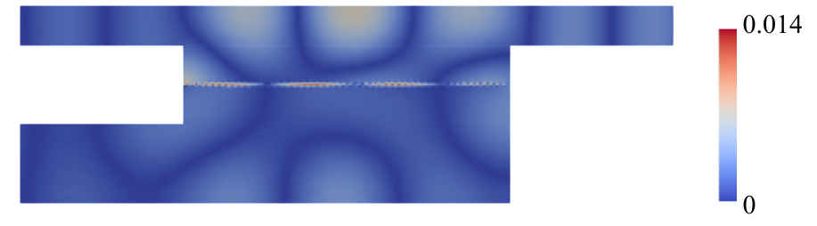
Figure 8 represents the distribution of e±e^{\pm}. Although large values of e±e^{\pm} can be found around Γ0\Gamma^{0} and at the corners of the geometries, they are less than 1.4%, and this supports the validity of the proposed homogenization method.

The proposed homogenization method assumes periodicity in the microscale problems, but periodicity is not assumed in the macroscale problem. If this discrepancy was significant, errors would have been observed in the solution of the homogenization method, owing to the rigid side walls at both ends of the transmission layer. However, such errors were not confirmed, as indicated by Fig. 8. This is because the unit cell size and the widths of the region where the unit cell is in contact with the outer boundaries are considerably smaller than the wavelength of the acoustic waves, and the structure of the metasurface can be replaced by a homogeneous material. In [52], this type of discrepancy caused by the finite length of a periodic structure was examined by using the method of matched asymptotic expansions. As this error appears to be small for the practical use of the proposed model, we neglect this point.

Refer to caption
Figure 7: Distribution of the real part of acoustic pressure at k0=25​[m−1]k_{0}=25~{\color[rgb]{0,0,0}\mathrm{[m^{-1}]}} for (a) Re⁡(P±)\mathrm{Re}(P^{\pm}) and (b) Re⁡(pR​e​f)\mathrm{Re}(p^{Ref}).
Refer to caption
Figure 8: Distribution of e±e^{\pm} at k0=25​[m−1]k_{0}=25~{\color[rgb]{0,0,0}\mathrm{[m^{-1}]}}.

7.2 Optimization results

Two numerical cases are solved to demonstrate the validity of the proposed optimization method. In case 1, the amplitude of acoustic pressure on Γout2\Gamma_{\mathrm{out2}} is minimized, whereas that on Γout1\Gamma_{\mathrm{out1}} is maximized. Here, we assign Γout2\Gamma_{\mathrm{out2}} to Γmin\Gamma_{\mathrm{min}} and Γout1\Gamma_{\mathrm{out1}} to Γmax\Gamma_{\mathrm{max}} in the objective functional expressed in Eq. (57). Case 2 is the inverse of case 1, that is, we assign Γout1\Gamma_{\mathrm{out1}} to Γmin\Gamma_{\mathrm{min}} and Γout2\Gamma_{\mathrm{out2}} to Γmax\Gamma_{\mathrm{max}}. The weighting factor ww in the objective functional was fixed at w=0.5w=0.5 for both cases. The computational domains in the macroscale and material properties in DD are set at the same values as those in section 7.1. To represent the macroscale system, 17,251 triangular elements are used, similar to the example shown in Fig. 5(b). However, approximately 20,000 elements are used for the microscale system. Details regarding the finite element discretization in the microscale are explained in Section 7.3. The wavenumber of the incident wave was set to k0=25​[m−1]k_{0}=25~{\color[rgb]{0,0,0}\mathrm{[m^{-1}]}} corresponding to 1369​[Hz]1369~\mathrm{[Hz]} and the corresponding wave amplitude was set to Pin=1​[Pa]P_{\mathrm{in}}=1~\mathrm{[Pa]}.

Figure 9(a) shows the settings of the computational domains at the microscale and the initial configuration in DD for both optimization cases. The black-colored domain represents Ωelastic\Omega_{\mathrm{elastic}} comprising aluminum, whereas the gray-colored domain represents Ωair\Omega_{\mathrm{air}}. A circular elastic domain was selected as an initial configuration, with a radius of 0.3{\color[rgb]{0,0,0}0.3} in the 𝒚\bm{y} coordinate. The other dimensions are listed in the figure. By solving the cell problems for the initial configuration at the microscale, the homogenized coefficients are evaluated as (A11∗,B1∗,K−1∗,F∗)=(0.466[m3kg−1],3.20×10−9,5.05×10−6[Pa−1],2.18[kgm−3])({A}_{11}^{\ast},{B}_{1}^{\ast},K^{-1\ast},F^{\ast})=(0.466~{\color[rgb]{0,0,0}\mathrm{[m^{3}~kg^{-1}]}},3.20\times 10^{-9},5.05\times 10^{-6}~{\color[rgb]{0,0,0}\mathrm{[Pa^{-1}]}},2.18~{\color[rgb]{0,0,0}\mathrm{[kg~m^{-3}]}}). The acoustic-wave propagation behavior in the macroscale is obtained using these values in the homogenized equations. Figure 9(b) shows the distribution of the real part of acoustic pressure at the initial configuration. To present the optimization results clearly, the upper and lower limits of the color bar of the contour diagram are fixed to 0.80.8 and −0.8​[Pa]-0.8\mathrm{[Pa]}, respectively, in order to emphasize the transmitted waves in the upper region of Ω−\Omega^{-}. Similarly, Fig. 9(c) shows the distribution of the absolute value of acoustic pressure. It is observed that |P−||P^{-}| around Γout1\Gamma_{\mathrm{out1}} exceeds that around Γout2\Gamma_{\mathrm{out2}}. Moreover, the squared norm of the acoustic pressure on Γout1\Gamma_{\mathrm{out1}} and Γout2\Gamma_{\mathrm{out2}} is 3.59×10⁻²​[Pa2​m]3.59\times 10^{-2}~[\mathrm{Pa}^{2}~\mathrm{m}] and 2.70×10⁻²​[Pa2​m]2.70\times 10^{-2}~[\mathrm{Pa}^{2}~\mathrm{m}], respectively. As in the definition of the objective functional, i.e., Eq. (57), these values were used for the normalization of JJ. According to this definition, the initial value of JJ is 00 with J1=J2=1J_{1}=J_{2}=1.

Refer to caption
Figure 9: (a) Computational domains and the initial configuration at the microscale. (b) Distribution of the real part of acoustic pressure, Re⁡(P±)\mathrm{Re}(P^{\pm}). (c) Distribution of the absolute value of acoustic pressure, |P±||P^{\pm}|.

Figure 10 represents the optimization results for case 1. The optimized configuration is shown in Fig. 10(a), and it is characterized by the striped structures tilted toward the left. The finite element discretization of the obtained design involves 26,264 elements, the details of which are explained in Section 7.3. This structure exhibits homogenized coefficients of (A11∗,B1∗,K−1∗,F∗)=({A}_{11}^{\ast},{B}_{1}^{\ast},K^{-1\ast},F^{\ast})=
(0.273​[m3​kg−1],−2.10,6.66×10−6​[Pa−1],10.14​[kg​m−3]){\color[rgb]{0,0,0}(0.273~{\color[rgb]{0,0,0}\mathrm{[m^{3}~kg^{-1}]}},-2.10,6.66\times 10^{-6}~{\color[rgb]{0,0,0}\mathrm{[Pa^{-1}]}},10.14~{\color[rgb]{0,0,0}\mathrm{[kg~m^{-3}]}})}. By using these values, the macroscopic acoustic-pressure distribution is obtained as shown in Fig. 10(b). The objective functional is calculated as J=−0.260J={\color[rgb]{0,0,0}-0.260} with J1=0.456J_{1}={\color[rgb]{0,0,0}0.456} and J2=0.975J_{2}={\color[rgb]{0,0,0}0.975}. In other words, the optimized result was obtained such that the amplitude of the acoustic pressure on Γout2\Gamma_{\mathrm{out2}} was reduced, whereas that of the pressure on Γout1\Gamma_{\mathrm{out1}} was retained. Figure 10(b) and (c) show this trend in the distribution of Re⁡(P−)\mathrm{Re}(P^{-}) and |P−||P^{-}|. Compared to the case of the initial configuration shown in Fig. 9(b) and (c), the amplitude appears small around the outlet, Γout2\Gamma_{\mathrm{out2}}. Figure 11 presents a history of the objective functional JJ with the intermediate and optimized designs. It was observed that a circular structure at the initial iteration was stretched to form the striped structures during optimization. The optimization calculation was halted at the 983rd iteration, where the 10-iteration moving average of the relative error between the values of JJ for two consecutive iterations was less than 3×10−43\times 10^{-4}. It is noted that the obtained design is dependent on the initial configuration. At the microscale, the periodic boundary condition is applied in the y1y_{1} direction; thus, the same performance as that of the optimized design is obtained for the shape translated along the y1y_{1} direction. If the position of the initial configuration is shifted, the optimized design will also be translated. Therefore, the optimized structure will change depending on the initial configuration.

By considering interface Γ0\Gamma^{0} in Fig. 10(b) and (c), a strong discontinuity in the acoustic pressure can be observed. To examine the details of this behavior around Γ0\Gamma^{0}, the reference solution is obtained for the entire system with an array of unit cells containing the optimized configuration, similar to that in section 7.1. Figure 12(a) presents the acoustic-pressure distribution for this reference analysis. The distribution is similar in the outer regions, Ω±\Omega^{\pm}, and demonstrates the validity of the proposed homogenization method. Around the unit cells, the pressure contour is distorted owing to the optimized configuration. Figure 12(b) provides additional details on the acoustic-wave-propagation behavior through the magnified view of the dotted box in Fig. 12(a). The green-colored arrows represent the sound intensity vector in air, as expressed by

𝑰=12​Re​(pR​e​f​𝒖R​e​f¯),\displaystyle\bm{I}=\frac{1}{2}\mathrm{Re}\left(p^{Ref}\overline{\bm{u}^{Ref}}\right),

where 𝒖R​e​f=−1i​ω​ρ0∇pR​e​f\bm{u}^{Ref}=-\frac{1}{i\omega\rho_{0}}\nabla p^{Ref} denotes the particle velocity, and 𝒖R​e​f¯\overline{\bm{u}^{Ref}} represents the complex conjugate of 𝒖R​e​f\bm{u}^{Ref}. The sound intensity vector, 𝑰\bm{I}, indicates the direction of energy flow. Within the unit cells, the direction of 𝑰\bm{I} is almost along the surface of the optimized configuration, and this results in a reduction of the transmission of acoustic waves toward outlet Γout2\Gamma_{\mathrm{out2}}.

Refer to caption
Figure 10: (a) Optimized configuration for case 1. (b) Distribution of the real part of acoustic pressure, Re⁡(P±)\mathrm{Re}(P^{\pm}). (c) Distribution of the absolute value of acoustic pressure, |P±||P^{\pm}|.
Refer to caption
Figure 11: History of objective functional JJ with the intermediate and optimized designs for case 1.
Refer to caption
Figure 12: (a) Distribution of the real part of acoustic pressure, Re⁡(pR​e​f)\mathrm{Re}(p^{Ref}), corresponding to the optimized configuration in case 1. (b) The magnified view of (a). The green-colored arrows represent the sound intensity vector, 𝑰\bm{I}, in air.

Figure 13 represents the optimization results for case 2. Similar to case 1, the optimized configuration shown in Fig. 13(a) is characterized by the striped structures, but these are tilted toward the right. The finite element discretization of the obtained design involves 21,182 elements, the details of which are explained in Section 7.3. The homogenized coefficients are evaluated as (A11∗,B1∗,K−1∗,F∗)=(0.234[m3kg−1],1.10,6.81×10−6[Pa−1],4.30[kgm−3])({A}_{11}^{\ast},{B}_{1}^{\ast},K^{-1\ast},F^{\ast})={\color[rgb]{0,0,0}(0.234~{\color[rgb]{0,0,0}\mathrm{[m^{3}~kg^{-1}]}},1.10,6.81\times 10^{-6}~{\color[rgb]{0,0,0}\mathrm{[Pa^{-1}]}},4.30~{\color[rgb]{0,0,0}\mathrm{[kg~m^{-3}]}})}, and the acoustic-pressure distribution at the macroscale is obtained, as shown in Fig. 13(b) and (c). Compared to the case of the initial configuration, as shown in Fig. 9(b), the amplitude of acoustic pressure around Γout1\Gamma_{\mathrm{out1}} was reduced, whereas that of the pressure around Γout1\Gamma_{\mathrm{out1}} increased with the use of the optimization formulation. Moreover, the value of objective functional JJ was −0.366{\color[rgb]{0,0,0}-0.366} with J1=0.718J_{1}={\color[rgb]{0,0,0}0.718} and J2=1.45J_{2}={\color[rgb]{0,0,0}1.45}; this implies that both the properties of the metasurface for maximizing and minimizing the amplitude of acoustic pressure were improved. Although the value of JJ was improved, a significant change in pressure distribution, as compared to case 1, could not be obtained. This was likely due to the settings of the computational domain in the macroscale and the objective functional. The value of the squared norm of the acoustic pressure on Γout1\Gamma_{\mathrm{out1}} exceeds that of the pressure on Γout2\Gamma_{\mathrm{out2}} during the initial configuration. Therefore, additional efforts are required to realize an opposite trend in pressure distribution than that in case 1. As the weighting factors in Eq. (57) were fixed during optimization and set to the same values as those in case 1, the optimization calculation did not proceed to realize such a significant change in pressure distribution.

Figure 14 represents a history of the objective functional JJ with the intermediate and optimized designs. An evolution behavior similar to that in case 1 was observed; however, the width of the striped structure during the initial iterations was less than that in case 1, which resulted in the unstable history of JJ, as compared to case 1. Consequently, we loosened the convergence criterion based on the moving average, and it was applied after the 900th iteration. The optimization calculation was halted at the 1156th iteration, where the 10-iteration moving average of the relative error between the values of JJ for two consecutive iterations was less than 8×10−48\times 10^{-4}.

For clear observations around interface Γ0\Gamma^{0}, we conducted the reference analysis for the entire system containing the optimized configuration. Figure 15(a) presents the acoustic-pressure distribution. As shown, the pressure contour is distorted owing to the optimized configuration, similar to that in case 1. Figure 15(b) shows the magnified view around the dotted box shown in Fig. 15(a). The direction of the sound intensity vector 𝑰\bm{I} is almost along the surface of the optimized configuration, and this reduces the transmission of acoustic waves toward outlet Γout1\Gamma_{\mathrm{out1}} and enables transmission toward Γout2\Gamma_{\mathrm{out2}}. Therefore, the mechanism of controlling the direction of wave propagation appears identical to that in case 1.

Refer to caption
Figure 13: (a) Optimized configuration for case 2. (b) Distribution of the real part of acoustic pressure, Re⁡(P±)\mathrm{Re}(P^{\pm}). (c) Distribution of the absolute value of acoustic pressure, |P±||P^{\pm}|.
Refer to caption
Figure 14: History of objective functional JJ with the intermediate and optimized designs for case 2.
Refer to caption
Figure 15: (a) Distribution of the real part of acoustic pressure, Re⁡(pR​e​f)\mathrm{Re}(p^{Ref}), corresponding to the optimized configuration in case 2. (b) The magnified view of (a). The green-colored arrows represent the sound intensity vector, 𝑰\bm{I}, in air.

These optimization results are summarized with the values of the homogenized coefficients and objective functional in Table 1. Among these coefficients, the most significant change can be observed in the value of coefficient B1∗{B}_{1}^{\ast} for both cases 1 and 2. Here, we discuss this change during the optimization. One of the homogenized equations in the macroscale containing coefficient B1∗{B}_{1}^{\ast} is described as follows:

∫Γ0(B1∗​∂p0∂x1−12​F∗​(G0++G0−))​ψ​d​Γx=1ϵ0​∫Γ0(P+−P−)​ψ​d​Γx​∀ψ∈L2​(Γ0).\displaystyle\int_{\Gamma^{0}}\left({B}_{1}^{\ast}\frac{\partial p^{0}}{\partial x_{1}}-\frac{1}{2}F^{\ast}(G_{0}^{+}+G_{0}^{-})\right)\psi d\Gamma_{x}=\frac{1}{\epsilon_{0}}\int_{\Gamma^{0}}({P}^{+}-{P}^{-})\psi d\Gamma_{x}~~~\forall\psi\in L^{2}(\Gamma^{0}). (79)

This equation implies that the jump between P±P^{\pm} on interface Γ0\Gamma^{0} depends on the values of B1∗{B}_{1}^{\ast} and F∗{F}^{\ast}. The left-hand side of Eq. (79) comprises two quantities concerning the gradient of acoustic pressure. The first quantity is the tangential derivative, ∂p0∂x1\frac{\partial p^{0}}{\partial x_{1}}, along interface Γ0\Gamma_{0}, while the second is G0±G_{0}^{\pm}, which has a relationship with the normal derivative to Γ0\Gamma^{0}, as indicated by the definition in Eq. (40). These gradient quantities are reflected in the jump denoted as (P+−P−)(P^{+}-P^{-}) on Γ0\Gamma^{0}, depending on the values of B1∗{B}_{1}^{\ast} and F∗{F}^{\ast}. In our setting of the optimization problem, the phase shift of acoustic pressure along Γ0\Gamma^{0} appears essential for minimizing the objective functional, based on the results shown in Figs. 12(b) and  15(b). The first term in Eq. (79), i.e., B1∗​∂p0∂x1{B}_{1}^{\ast}\frac{\partial p^{0}}{\partial x_{1}}, plays an important role as the tangential gradient represents the phase shift along Γ0\Gamma^{0}. The sign of B1∗{B}_{1}^{\ast} determines the direction of the phase shift along Γ0\Gamma^{0}; this can be observed in our optimization results. In case 1, the phase shift to the left can be confirmed across Γ0\Gamma^{0} from Ω+\Omega^{+} to Ω−\Omega^{-}, as shown in Fig. 12(b), where the sign of B1∗{B}_{1}^{\ast} is negative. By contrast, in the case 2, the phase shifts to the right across Γ0\Gamma^{0}, as shown in Fig. 15(b), where the sign of B1∗{B}_{1}^{\ast} is positive. Therefore, we consider that the optimization calculation proceeded such that the desired phase shift that minimizes the objective functional can be obtained by adjusting the value of B1∗{B}_{1}^{\ast}.

Table 1: Values of the homogenized coefficients and objective functional.
Initial configuration
Case 1
Case 2
A11∗​[m3​kg−1]{A}_{11}^{\ast}~{\color[rgb]{0,0,0}\mathrm{[m^{3}~kg^{-1}]}} 0.4660.466 0.2730.273 0.2340.234
B1∗{B}_{1}^{\ast} 3.20×10−93.20\times 10^{-9} −2.10-2.10 1.101.10
K−1∗[Pa−1]K^{-1\ast}~{\color[rgb]{0,0,0}\mathrm{[Pa^{-1}]}} 5.05×10−65.05\times 10^{-6} 6.66×10−66.66\times 10^{-6} 6.81×10−66.81\times 10^{-6}
F∗​[kg​m−3]F^{\ast}~{\color[rgb]{0,0,0}\mathrm{[kg~m^{-3}]}} 2.182.18 10.1410.14 4.304.30
JJ 00 −0.260-0.260 −0.366-0.366
J1J_{1} 11 0.4560.456 0.7180.718
J2J_{2} 11 0.9750.975 1.451.45

7.3 Mesh dependency of optimized designs

Refer to caption
Figure 16: Optimized results with different finite element discretization: (a) Case 1 with 26,264 elements, (b) Case 1 with 76,406 elements, (c) Case 2 with 21,182 elements, and (d) Case 2 with 63,100 elements.

To examine the mesh dependency of the optimized designs, optimization calculations are conducted for case 1 and 2 using finer meshes in the microscale systems than those used for the results shown in Fig. 10 and Fig. 13. Figure 16 shows a comparison of the obtained configurations with finite element discretization. The previous results for case 1 and 2 are shown in Fig. 16(a) and (c), respectively. Figure 16(b) and (d) present the optimized results for case 1 and 2 when using the finer meshes, respectively. The total number of elements in (b) is 76,406, whereas that in (d) is 63,100. These are roughly three times more than those used for the previous results. All the designs are characterized by striped structures, and there appears to be no difference between the results. As the objective functional in Eq. (57) aims to simultaneously maximize and minimize the amplitude of the transmitted wave at different outlets, it is deduced that the striped structures with a certain finite width are required for each case. Therefore, low mesh dependency is observed for the optimized designs.

7.4 Discussion about computational cost

Here, the computational effort required in the proposed method is presented. As the proposed homogenization method decomposes the entire system of the metasurface into the macroscale and microscale, the total degree of freedom (DOF) required to analyze the system can be reduced. Let DOF⁡(u)\mathrm{DOF}(u) denote the number of DOF for a variable uu in the FEM. The total number of the DOF per single optimization loop, DOFh​o​m\mathrm{DOF}_{hom}, can be estimated as follows:

DOFh​o​m={DOF⁡(η)+DOF⁡(ξ)+DOF⁡(ϕ)}+∑i=15DOF⁡(um​a​c​r​oi)+∑i=15DOF⁡(vm​a​c​r​oi),\displaystyle\mathrm{DOF}_{hom}=\{\mathrm{DOF}(\eta)+\mathrm{DOF}(\xi)+\mathrm{DOF}(\phi)\}+\sum_{i=1}^{5}\mathrm{DOF}(u_{macro}^{i})+\sum_{i=1}^{5}\mathrm{DOF}(v_{macro}^{i}),

where 𝒖m​a​c​r​o=(p0,P+,P−,G0+,G0−)\bm{u}_{macro}=(p^{0},P^{+},P^{-},G_{0}^{+},G_{0}^{-}) represents the state variables in the macroscale, whereas 𝒗m​a​c​r​o=(q0,Q+,Q−,Ψ0+,Ψ0−)\bm{v}_{macro}=(q^{0},Q^{+},Q^{-},\Psi_{0}^{+},\Psi_{0}^{-}) represents the adjoint variables in the macroscale. To determine the efficiency of the proposed homogenization model, we calculate the DOF of the system of the metasurface, whose unit cell structure is the same as that in the initial configuration, shown in Fig. 9(a). Figure 17 presents the finite element discretization in the microscale, where 21,360 triangular elements are used. For the macroscale, we use the same discretization as discussed in Section 7.2. The DOF for each variable in this system is calculated and summarized in Table 2. Based on Table 2 and the abovementioned equation, DOFh​o​m\mathrm{DOF}_{hom} is estimated as 167,512.

Refer to caption
Figure 17: Finite element discretization for the microscale system with 21,360 elements.
Table 2: Degree of freedom (DOF) required in the FEM for the initial iteration of the proposed optimization method.
Variables
DOF
Micro- (η,ξ)({\eta},{\xi}) (43361,43361)(43361,43361)
scale ϕ\phi 92269226
Macro- (p0,P+,P−,G0+,G0−)(p^{0},P^{+},P^{-},G_{0}^{+},G_{0}^{-}) (201,17474,17905,101,101)(201,17474,17905,101,101)
scale (q0,Q+,Q−,Ψ0+,Ψ0−)(q^{0},Q^{+},Q^{-},\Psi_{0}^{+},\Psi_{0}^{-}) (201,17474,17905,101,101)(201,17474,17905,101,101)

In the case without homogenization, the DOF is estimated as a sum of the DOF of the state variable, adjoint variable corresponding to 𝒗m​a​c​r​o{\bm{v}}_{macro}, and level set function for representing the material distribution in the layer of the metasurface. To estimate this, a reference analysis is introduced in Section 7.1. In other words, we arrayed 50 unit cells over the transmission layer; the finite element discretization in each unit cell is depicted in Fig. 17. To represent the entire system, 1,847,847 triangular elements were required. Under this setting, the total DOF of the reference analysis, DOFr​e​f\mathrm{DOF}_{ref}, is estimated as 7,854,809, which is approximately 47 times larger than DOFh​o​m\mathrm{DOF}_{hom}. The DOF reduction afforded by the proposed method is attributable to the small number of finite elements required for solving the macroscale system.

This reduction in the DOF resulted in a shorter computational time than that required for the standard FEM. The computational time required for obtaining the state variables at the initial iteration by using the proposed method is compared with that for the conventional FEM without homogenization. The discretization conditions are the same as those explained above. We used a desktop computer (Intel Core i9 CPU 3.6 GHz, 10 cores, 128 GB memory) for both analyses, and their FEM implementation is based on FreeFEM. The computational time for (η,ξ)(\eta,\xi) in a unit cell was 0.59 [s], whereas that for (p0,P+,P−,G0+,G0−)(p^{0},P^{+},P^{-},G_{0}^{+},G_{0}^{-}) in the macroscale was 0.58 [s]. Subsequently, the total computational time for the state variables per optimization loop could be estimated as 1.17 [s]. By contrast, the reference analysis without homogenization required 108.88 [s]. Based on this comparison, we concluded that the proposed method can analyze the system of the metasurface efficiently, with less computational cost than that of the standard FEM, which is beneficial for optimization.

Although we targeted two-dimensional metasurfaces that function at a single frequency, it is expected that the proposed method can be extended to three-dimensional or multi-frequency problems. The efficiency of the proposed method is apparent in the case of multi-frequency optimizations. As the microscale problem is independent of frequency, we only need to solve the microscale system once. Although the macroscale analysis requires iterations with various input frequencies, it needs considerably less computational time than the conventional FEM, as evidenced by the abovementioned example. The proposed homogenization method is also suitable for three-dimensional problems, as explained in Section 2. The number of cell problems increases to three, whereas the two-dimensional case involves two. Furthermore, the homogenized equations are defined in the three-dimensional external regions Ω±\Omega^{\pm} and the two-dimensional surface Γ0\Gamma^{0}, whereas those for the abovementioned results are defined in the two-dimensional external regions Ω±\Omega^{\pm} and one-dimensional boundary Γ0\Gamma^{0}. This will increase the computational costs; however, the standard FEM also requires a larger number of finite elements to analyze such a system. If the metasurface is composed of a periodic array of unit cells with complex structures, the DOF without homogenization will be significantly higher than that in the case with homogenization. Thus, the proposed method will require less computational time.

8 Conclusion

In this paper, we proposed a topology optimization method for the design of acoustic metasurfaces based on the homogenization method. We summarize the results of this study as follows:

  1. 1.

    This study introduces a homogenization method for acoustic metasurfaces based on the method proposed by Rohan and Lukeš [38, 39]. We extend their approach to a metasurface system comprising both acoustic and elastic media. The proposed method can decompose the entire metasurface system, including the complex structures of unit cells, into problems defined at the microscale and macroscale. The microscale problem involves the so-called cell problem defined in the unit cell with appropriate periodic boundary conditions, and the homogenized coefficients expressing the feature of the unit cell can be estimated by solving the cell problems. The macroscale problem is defined in all regions, except the domain formed by the array of unit cells. The complex structure of the metasurface is replaced with a boundary comprising the homogenized coefficients, and this reduces the computational costs.

  2. 2.

    An optimization problem was formulated within the framework of the proposed homogenization method, and it includes a level set-based topology optimization. Acoustic responses at the macroscale were set to the objective functional, and the material distribution at the microscale was optimized to minimize the objective functional. As a typical macroscopic response, we chose the amplitude of transmitted acoustic waves at a certain target frequency and set them to the objective functional.

  3. 3.

    A sensitivity analysis was conducted based on the concept of the topological derivative. We used the topological-shape sensitivity method to derive the topological derivative, which contains contributions at the macroscale and microscale of the objective functional. The macroscale contribution can be estimated by solving the state and adjoint equations at the macroscale, whereas the microscale contribution can be obtained by solving the cell problems.

  4. 4.

    An optimization algorithm that incorporates the homogenization method and the level set-based topology optimization method was proposed. In addition, we noted some numerical treatments to implement the algorithm using an FEM, especially for the selected shape functions and mesh refinement using the level set function.

  5. 5.

    Numerical examples were provided to confirm the validity of the proposed method. First, we provided an example that supports the validity of the proposed homogenization method and compared the solutions with those obtained using the standard FEM (without homogenization); good congruence was observed between both, except for the resonance frequency. Then, we optimized both results, which were examined with respect to the settings of the objective functional. In both cases, each optimized configuration was characterized by striped structures of the elastic medium. In addition, phase shifts were observed around the array of unit cells, which play a key role in minimizing the objective functional.

Although our optimization results target a single frequency, the method can be extended to include a range of frequencies by considering such a range in the settings of the objective functional. A three-dimensional optimization problem can also be addressed, as the homogenization method is valid three-dimensionally, as discussed in [41, 39]. Furthermore, our method could help in the optimum design of graded metasurfaces, which correspond to the spatial distribution of the homogenized coefficients at the macroscale. In this research, the design variable was restricted to the material distribution at the microscale; however, if the distribution of the homogenized coefficients at the macroscale is also considered as the design variable, the design space could be increased, and more effective control over acoustic waves could be realized. We plan to achieve these extensions in our future research.

Acknowledgment

Funding: This work was supported in part by JSPS KAKENHI [grant number 20K14636] and Ono Charitable Trust for Acoustics.

We would like to thank Editage (www.editage.com) for English language editing.

Appendix A Details for deriving the homogenized equations

In this section, additional details on obtaining the homogenized equations in Section 2 are explained.

First, the procedure to obtain Eq. (23) is provided. By substituting the convergence results for acoustic pressure, as expressed in Eqs. (20)–(22), and corresponding test function into the weak form [Eq. (16)], we obtain

∫Γ0−∫Y1ρ⁡(𝒚)(∇¯xp0+∇¯yp1)⋅(∇¯xq0+∇¯yq1)dΩydΓx+∫Γ0−∫Y1ρ⁡(𝒚)∂p1∂z∂q1∂zdΩydΓx\displaystyle\int_{\Gamma^{0}}\mathchoice{{\vbox{\hbox{$\textstyle-$ }}\kern-7.83337pt}}{{\vbox{\hbox{$\scriptstyle-$ }}\kern-6.11674pt}}{{\vbox{\hbox{$\scriptscriptstyle-$ }}\kern-5.48965pt}}{{\vbox{\hbox{$\scriptscriptstyle-$ }}\kern-5.31259pt}}\!\int_{Y}\frac{1}{\rho(\bm{y})}(\overline{\nabla}_{x}p^{0}+\overline{\nabla}_{y}p^{1})\cdot(\overline{\nabla}_{x}q^{0}+\overline{\nabla}_{y}q^{1})d\Omega_{y}d\Gamma_{x}+\int_{\Gamma^{0}}\mathchoice{{\vbox{\hbox{$\textstyle-$ }}\kern-7.83337pt}}{{\vbox{\hbox{$\scriptstyle-$ }}\kern-6.11674pt}}{{\vbox{\hbox{$\scriptscriptstyle-$ }}\kern-5.48965pt}}{{\vbox{\hbox{$\scriptscriptstyle-$ }}\kern-5.31259pt}}\!\int_{Y}\frac{1}{\rho(\bm{y})}\frac{\partial p^{1}}{\partial z}\frac{\partial q^{1}}{\partial z}d\Omega_{y}d\Gamma_{x}
−∫Γ0−∫Yω2K⁡(𝒚)p0q0dΩydΓx=−∫Γ0{q0−∫ΘΔg1+g0(−∫Iy+q1−−∫Iy−q1)}dΓydΓx,\displaystyle-\int_{\Gamma^{0}}\mathchoice{{\vbox{\hbox{$\textstyle-$ }}\kern-7.83337pt}}{{\vbox{\hbox{$\scriptstyle-$ }}\kern-6.11674pt}}{{\vbox{\hbox{$\scriptscriptstyle-$ }}\kern-5.48965pt}}{{\vbox{\hbox{$\scriptscriptstyle-$ }}\kern-5.31259pt}}\!\int_{Y}\frac{\omega^{2}}{K(\bm{y})}p^{0}q^{0}d\Omega_{y}d\Gamma_{x}=-\int_{\Gamma^{0}}\left\{q^{0}\mathchoice{{\vbox{\hbox{$\textstyle-$ }}\kern-7.83337pt}}{{\vbox{\hbox{$\scriptstyle-$ }}\kern-6.11674pt}}{{\vbox{\hbox{$\scriptscriptstyle-$ }}\kern-5.48965pt}}{{\vbox{\hbox{$\scriptscriptstyle-$ }}\kern-5.31259pt}}\!\int_{\Theta}\Delta g^{1}+g^{0}(\mathchoice{{\vbox{\hbox{$\textstyle-$ }}\kern-7.83337pt}}{{\vbox{\hbox{$\scriptstyle-$ }}\kern-6.11674pt}}{{\vbox{\hbox{$\scriptscriptstyle-$ }}\kern-5.48965pt}}{{\vbox{\hbox{$\scriptscriptstyle-$ }}\kern-5.31259pt}}\!\int_{I_{y}^{+}}q^{1}-\mathchoice{{\vbox{\hbox{$\textstyle-$ }}\kern-7.83337pt}}{{\vbox{\hbox{$\scriptstyle-$ }}\kern-6.11674pt}}{{\vbox{\hbox{$\scriptscriptstyle-$ }}\kern-5.48965pt}}{{\vbox{\hbox{$\scriptscriptstyle-$ }}\kern-5.31259pt}}\!\int_{I_{y}^{-}}q^{1})\right\}d\Gamma_{y}d\Gamma_{x}, (80)

where Θ\Theta represents the mid-plane of the unit cell, as shown in Fig. 1(b). −∫=1|Θ|∫\mathchoice{{\vbox{\hbox{$\textstyle-$ }}\kern-7.83337pt}}{{\vbox{\hbox{$\scriptstyle-$ }}\kern-6.11674pt}}{{\vbox{\hbox{$\scriptscriptstyle-$ }}\kern-5.48965pt}}{{\vbox{\hbox{$\scriptscriptstyle-$ }}\kern-5.31259pt}}\!\int=\frac{1}{|\Theta|}\int is defined as an operator that averages the integrand over the cross-sectional area of the unit cell, |Θ||\Theta|. Δ​g1\Delta g^{1} is used to express the difference between g1±g^{1\pm} as Δ​g1=g1+−g1−\Delta g^{1}=g^{1+}-g^{1-}.

Next, we derive the so-called cell problems defined in YY. By setting the test functions as q0=0q^{0}=0 and q1≠0q^{1}\neq 0, the following equation is obtained:

∫Γ0−∫Y1ρ⁡(𝒚)(∇¯yp1⋅∇¯yq1+∂p1∂z∂q1∂z)dΩydΓx\displaystyle\int_{\Gamma^{0}}\mathchoice{{\vbox{\hbox{$\textstyle-$ }}\kern-7.83337pt}}{{\vbox{\hbox{$\scriptstyle-$ }}\kern-6.11674pt}}{{\vbox{\hbox{$\scriptscriptstyle-$ }}\kern-5.48965pt}}{{\vbox{\hbox{$\scriptscriptstyle-$ }}\kern-5.31259pt}}\!\int_{Y}\frac{1}{\rho(\bm{y})}\left(\overline{\nabla}_{y}p^{1}\cdot\overline{\nabla}_{y}q^{1}+\frac{\partial p^{1}}{\partial z}\frac{\partial q^{1}}{\partial z}\right)d\Omega_{y}d\Gamma_{x}
=−∫Γ0∇¯xp0⋅(−∫Y1ρ⁡(𝒚)∇¯yq1)dΩydΓx−∫Γ0g0(−∫Iy+q1−−∫Iy−q1)dΓydΓx.\displaystyle=-\int_{\Gamma^{0}}\overline{\nabla}_{x}p^{0}\cdot\left(\mathchoice{{\vbox{\hbox{$\textstyle-$ }}\kern-7.83337pt}}{{\vbox{\hbox{$\scriptstyle-$ }}\kern-6.11674pt}}{{\vbox{\hbox{$\scriptscriptstyle-$ }}\kern-5.48965pt}}{{\vbox{\hbox{$\scriptscriptstyle-$ }}\kern-5.31259pt}}\!\int_{Y}\frac{1}{\rho(\bm{y})}\overline{\nabla}_{y}q^{1}\right)d\Omega_{y}d\Gamma_{x}-\int_{\Gamma^{0}}g^{0}\left(\mathchoice{{\vbox{\hbox{$\textstyle-$ }}\kern-7.83337pt}}{{\vbox{\hbox{$\scriptstyle-$ }}\kern-6.11674pt}}{{\vbox{\hbox{$\scriptscriptstyle-$ }}\kern-5.48965pt}}{{\vbox{\hbox{$\scriptscriptstyle-$ }}\kern-5.31259pt}}\!\int_{I_{y}^{+}}q^{1}-\mathchoice{{\vbox{\hbox{$\textstyle-$ }}\kern-7.83337pt}}{{\vbox{\hbox{$\scriptstyle-$ }}\kern-6.11674pt}}{{\vbox{\hbox{$\scriptscriptstyle-$ }}\kern-5.48965pt}}{{\vbox{\hbox{$\scriptscriptstyle-$ }}\kern-5.31259pt}}\!\int_{I_{y}^{-}}q^{1}\right)d\Gamma_{y}d\Gamma_{x}. (81)

This equation can be regarded as a weak form of the unknown, p1p^{1}. Owing to linearity, p1p^{1} is expressed as

p1​(𝒙′,𝒚)=∑α=1N−1(ηα​(𝒚)​∂p0∂xα​(𝒙′))+ξ⁡(𝒚)​g0​(𝒙′),\displaystyle p^{1}(\bm{x^{\prime}},\bm{y})=\sum_{\alpha=1}^{N-1}\left({\color[rgb]{0,0,0}\eta}^{\alpha}(\bm{y})\frac{\partial p^{0}}{\partial x_{\alpha}}(\bm{x^{\prime}})\right)+\xi(\bm{y})g^{0}(\bm{x^{\prime}}), (82)

where the functions ηα{\color[rgb]{0,0,0}\eta}^{\alpha} and ξ\xi are the solutions of the cell problems in Eq. (27) and (28).

Next, the macroscale problem defined on Γ0\Gamma_{0} is derived by substituting q0≠0q^{0}\neq 0 and q1=0q^{1}=0 into the weak form [Eq. (16)] as follows:

∫Γ0−∫Y1ρ⁡(𝒚)(∇¯xp0+∇¯yp1)⋅∇¯xq0dΩydΓx−∫Γ0−∫Yω2K⁡(𝒚)p0q0dΩydΓx\displaystyle\int_{\Gamma^{0}}\mathchoice{{\vbox{\hbox{$\textstyle-$ }}\kern-7.83337pt}}{{\vbox{\hbox{$\scriptstyle-$ }}\kern-6.11674pt}}{{\vbox{\hbox{$\scriptscriptstyle-$ }}\kern-5.48965pt}}{{\vbox{\hbox{$\scriptscriptstyle-$ }}\kern-5.31259pt}}\!\int_{Y}\frac{1}{\rho(\bm{y})}(\overline{\nabla}_{x}p^{0}+\overline{\nabla}_{y}p^{1})\cdot\overline{\nabla}_{x}q^{0}d\Omega_{y}d\Gamma_{x}-\int_{\Gamma^{0}}\mathchoice{{\vbox{\hbox{$\textstyle-$ }}\kern-7.83337pt}}{{\vbox{\hbox{$\scriptstyle-$ }}\kern-6.11674pt}}{{\vbox{\hbox{$\scriptscriptstyle-$ }}\kern-5.48965pt}}{{\vbox{\hbox{$\scriptscriptstyle-$ }}\kern-5.31259pt}}\!\int_{Y}\frac{\omega^{2}}{K(\bm{y})}p^{0}q^{0}d\Omega_{y}d\Gamma_{x}
=−∫Γ0q0(−∫ΘΔq1)dΓydΓx\displaystyle=-\int_{\Gamma^{0}}q^{0}\left(\mathchoice{{\vbox{\hbox{$\textstyle-$ }}\kern-7.83337pt}}{{\vbox{\hbox{$\scriptstyle-$ }}\kern-6.11674pt}}{{\vbox{\hbox{$\scriptscriptstyle-$ }}\kern-5.48965pt}}{{\vbox{\hbox{$\scriptscriptstyle-$ }}\kern-5.31259pt}}\!\int_{\Theta}\Delta q^{1}\right)d\Gamma_{y}d\Gamma_{x} (83)

By using the expression of p1p^{1}, this equation can be modified as

∑α=1N−1∑β=1N−1∫Γ0∂p0∂xβ∂q0∂xα[−∫Y1ρ⁡(𝒚){∇¯y(ηβ+yβ)⋅∇¯y(ηα+yα)+∂ηβ∂z∂ηα∂z}dΩy]dΓx\displaystyle\sum_{\alpha=1}^{N-1}\sum_{\beta=1}^{N-1}\int_{\Gamma^{0}}\frac{\partial p^{0}}{\partial x_{\beta}}\frac{\partial q^{0}}{\partial x_{\alpha}}\left[\mathchoice{{\vbox{\hbox{$\textstyle-$ }}\kern-7.83337pt}}{{\vbox{\hbox{$\scriptstyle-$ }}\kern-6.11674pt}}{{\vbox{\hbox{$\scriptscriptstyle-$ }}\kern-5.48965pt}}{{\vbox{\hbox{$\scriptscriptstyle-$ }}\kern-5.31259pt}}\!\int_{Y}\frac{1}{\rho(\bm{y})}\left\{\overline{\nabla}_{y}({\color[rgb]{0,0,0}\eta}^{\beta}+y_{\beta})\cdot\overline{\nabla}_{y}({\color[rgb]{0,0,0}\eta}^{\alpha}+y_{\alpha})+\frac{\partial{\color[rgb]{0,0,0}\eta}^{\beta}}{\partial z}\frac{\partial{\color[rgb]{0,0,0}\eta}^{\alpha}}{\partial z}\right\}d\Omega_{y}\right]d\Gamma_{x}
+∫Γ0g0∇¯xq0⋅(−∫Y1ρ⁡(𝒚)∇¯yξdΩy)dΓx−ω2∫Γ0p0q0(−∫Y1K⁡(𝒚)dΩy)dΓx\displaystyle+\int_{\Gamma^{0}}g^{0}\overline{\nabla}_{x}q^{0}\cdot\left(\mathchoice{{\vbox{\hbox{$\textstyle-$ }}\kern-7.83337pt}}{{\vbox{\hbox{$\scriptstyle-$ }}\kern-6.11674pt}}{{\vbox{\hbox{$\scriptscriptstyle-$ }}\kern-5.48965pt}}{{\vbox{\hbox{$\scriptscriptstyle-$ }}\kern-5.31259pt}}\!\int_{Y}\frac{1}{\rho(\bm{y})}\overline{\nabla}_{y}\xi d\Omega_{y}\right)d\Gamma_{x}-\omega^{2}\int_{\Gamma^{0}}p^{0}q^{0}\left(\mathchoice{{\vbox{\hbox{$\textstyle-$ }}\kern-7.83337pt}}{{\vbox{\hbox{$\scriptstyle-$ }}\kern-6.11674pt}}{{\vbox{\hbox{$\scriptscriptstyle-$ }}\kern-5.48965pt}}{{\vbox{\hbox{$\scriptscriptstyle-$ }}\kern-5.31259pt}}\!\int_{Y}\frac{1}{K(\bm{y})}d\Omega_{y}\right)d\Gamma_{x}
=−∫Γ0q0(−∫ΘΔg1dΓy)dΓx.\displaystyle=-\int_{\Gamma^{0}}q^{0}\left(\mathchoice{{\vbox{\hbox{$\textstyle-$ }}\kern-7.83337pt}}{{\vbox{\hbox{$\scriptstyle-$ }}\kern-6.11674pt}}{{\vbox{\hbox{$\scriptscriptstyle-$ }}\kern-5.48965pt}}{{\vbox{\hbox{$\scriptscriptstyle-$ }}\kern-5.31259pt}}\!\int_{\Theta}\Delta g^{1}d\Gamma_{y}\right)d\Gamma_{x}. (84)

By using the homogenized coefficients expressed with Eqs. (24)–(26), Eq. (84) can be rewritten as Eq. (23).

Next, the procedure to obtain Eq. (30) is explained. Using the mapped acoustic pressures defined in Eq. (31), the left-hand side of Eq. (29) can be considered for the mid-plane of Γ0\Gamma_{0}. The introduction of the scaled coordinate, z=xdϵz=\frac{x_{d}}{\epsilon}, and the multiplication of Eq. (29) with 1ϵ\frac{1}{\epsilon} yield

1ϵ​∫Γ0(Pm−−Pm+)​ψ​𝑑Γ=∫Γ0ψ​∫−κ2κ21ϵ​∂pϵ∂z​𝑑Γ.\displaystyle\frac{1}{\epsilon}\int_{\Gamma^{0}}({P}^{-}_{m}-{P}^{+}_{m})\psi d\Gamma=\int_{\Gamma^{0}}\psi\int_{-\frac{\kappa}{2}}^{\frac{\kappa}{2}}\frac{1}{\epsilon}\frac{\partial p^{\epsilon}}{\partial z}d\Gamma. (85)

Considering limit ϵ→0\epsilon\to 0, the right-hand side of Eq. (85) takes the following form:

∫Γ0ψ​∫−κ2κ21ϵ​∂pϵ∂z​𝑑Γ\displaystyle\int_{\Gamma^{0}}\psi\int_{-\frac{\kappa}{2}}^{\frac{\kappa}{2}}\frac{1}{\epsilon}\frac{\partial p^{\epsilon}}{\partial z}d\Gamma →∫Γ0ψ∫−κ2κ21ϵ(−∫Θ∂Tϵ​(pϵ)∂zdΓy)dzdΓx\displaystyle\to\int_{\Gamma^{0}}\psi\int_{-\frac{\kappa}{2}}^{\frac{\kappa}{2}}\frac{1}{\epsilon}\left(\mathchoice{{\vbox{\hbox{$\textstyle-$ }}\kern-7.83337pt}}{{\vbox{\hbox{$\scriptstyle-$ }}\kern-6.11674pt}}{{\vbox{\hbox{$\scriptscriptstyle-$ }}\kern-5.48965pt}}{{\vbox{\hbox{$\scriptscriptstyle-$ }}\kern-5.31259pt}}\!\int_{\Theta}\frac{\partial T_{\epsilon}(p^{\epsilon})}{\partial z}d\Gamma_{y}\right)dzd\Gamma_{x}
=∫Γ0ψ∫−κ2κ2−∫Θ∂p1∂zdΓydzdΓx\displaystyle=\int_{\Gamma^{0}}\psi\int_{-\frac{\kappa}{2}}^{\frac{\kappa}{2}}\mathchoice{{\vbox{\hbox{$\textstyle-$ }}\kern-7.83337pt}}{{\vbox{\hbox{$\scriptstyle-$ }}\kern-6.11674pt}}{{\vbox{\hbox{$\scriptscriptstyle-$ }}\kern-5.48965pt}}{{\vbox{\hbox{$\scriptscriptstyle-$ }}\kern-5.31259pt}}\!\int_{\Theta}\frac{\partial p^{1}}{\partial z}d\Gamma_{y}dzd\Gamma_{x}
=∫Γ0ψ−∫Y∂p1∂z​d​Ωy​d​Γx\displaystyle=\int_{\Gamma^{0}}\psi\mathchoice{{\vbox{\hbox{$\textstyle-$ }}\kern-7.83337pt}}{{\vbox{\hbox{$\scriptstyle-$ }}\kern-6.11674pt}}{{\vbox{\hbox{$\scriptscriptstyle-$ }}\kern-5.48965pt}}{{\vbox{\hbox{$\scriptscriptstyle-$ }}\kern-5.31259pt}}\!\int_{Y}\frac{\partial p^{1}}{\partial z}d\Omega_{y}d\Gamma_{x}
=∫Γ0ψ(−∫Iy−p1dΓy−−∫Iy+p1dΓy)dΓx\displaystyle=\int_{\Gamma^{0}}\psi\left(\mathchoice{{\vbox{\hbox{$\textstyle-$ }}\kern-7.83337pt}}{{\vbox{\hbox{$\scriptstyle-$ }}\kern-6.11674pt}}{{\vbox{\hbox{$\scriptscriptstyle-$ }}\kern-5.48965pt}}{{\vbox{\hbox{$\scriptscriptstyle-$ }}\kern-5.31259pt}}\!\int_{I_{y}^{-}}p^{1}d\Gamma_{y}-\mathchoice{{\vbox{\hbox{$\textstyle-$ }}\kern-7.83337pt}}{{\vbox{\hbox{$\scriptstyle-$ }}\kern-6.11674pt}}{{\vbox{\hbox{$\scriptscriptstyle-$ }}\kern-5.48965pt}}{{\vbox{\hbox{$\scriptscriptstyle-$ }}\kern-5.31259pt}}\!\int_{I_{y}^{+}}p^{1}d\Gamma_{y}\right)d\Gamma_{x}
=∫Γ0ψ∑α=1N−1∂p0∂xα(−∫Iy−ηαdΓy−−∫Iy+ηαdΓy)dΓx\displaystyle=\int_{\Gamma^{0}}\psi\sum_{\alpha=1}^{N-1}\frac{\partial p^{0}}{\partial x_{\alpha}}\left(\mathchoice{{\vbox{\hbox{$\textstyle-$ }}\kern-7.83337pt}}{{\vbox{\hbox{$\scriptstyle-$ }}\kern-6.11674pt}}{{\vbox{\hbox{$\scriptscriptstyle-$ }}\kern-5.48965pt}}{{\vbox{\hbox{$\scriptscriptstyle-$ }}\kern-5.31259pt}}\!\int_{I_{y}^{-}}{\color[rgb]{0,0,0}\eta}^{\alpha}d\Gamma_{y}-\mathchoice{{\vbox{\hbox{$\textstyle-$ }}\kern-7.83337pt}}{{\vbox{\hbox{$\scriptstyle-$ }}\kern-6.11674pt}}{{\vbox{\hbox{$\scriptscriptstyle-$ }}\kern-5.48965pt}}{{\vbox{\hbox{$\scriptscriptstyle-$ }}\kern-5.31259pt}}\!\int_{I_{y}^{+}}{\color[rgb]{0,0,0}\eta}^{\alpha}d\Gamma_{y}\right)d\Gamma_{x}
+∫Γ0ψg0(−∫Iy−ξdΓy−−∫Iy+ξdΓy)dΓx.\displaystyle+\int_{\Gamma^{0}}\psi g^{0}\left(\mathchoice{{\vbox{\hbox{$\textstyle-$ }}\kern-7.83337pt}}{{\vbox{\hbox{$\scriptstyle-$ }}\kern-6.11674pt}}{{\vbox{\hbox{$\scriptscriptstyle-$ }}\kern-5.48965pt}}{{\vbox{\hbox{$\scriptscriptstyle-$ }}\kern-5.31259pt}}\!\int_{I_{y}^{-}}\xi d\Gamma_{y}-\mathchoice{{\vbox{\hbox{$\textstyle-$ }}\kern-7.83337pt}}{{\vbox{\hbox{$\scriptstyle-$ }}\kern-6.11674pt}}{{\vbox{\hbox{$\scriptscriptstyle-$ }}\kern-5.48965pt}}{{\vbox{\hbox{$\scriptscriptstyle-$ }}\kern-5.31259pt}}\!\int_{I_{y}^{+}}\xi d\Gamma_{y}\right)d\Gamma_{x}. (86)

To obtain the last line, the expression of p1p^{1} is used. Furthermore, the homogenized coefficient F∗F^{\ast}, expressed by Eq. (32), was introduced, and 𝑩∗\bm{B}^{\ast} was modified using the weak forms of the cell problems as follows:

Bα∗\displaystyle B^{\ast}_{\alpha} =−∫Y1ρ⁡(𝒚)∂ξ∂yαdΩy\displaystyle=\mathchoice{{\vbox{\hbox{$\textstyle-$ }}\kern-7.83337pt}}{{\vbox{\hbox{$\scriptstyle-$ }}\kern-6.11674pt}}{{\vbox{\hbox{$\scriptscriptstyle-$ }}\kern-5.48965pt}}{{\vbox{\hbox{$\scriptscriptstyle-$ }}\kern-5.31259pt}}\!\int_{Y}\frac{1}{\rho(\bm{y})}\frac{\partial\xi}{\partial y_{\alpha}}d\Omega_{y}
=−−∫Y1ρ⁡(𝒚)(∇¯yξ⋅∇¯yηα+∂ξ∂z∂ηα∂z)dΩy\displaystyle=-\mathchoice{{\vbox{\hbox{$\textstyle-$ }}\kern-7.83337pt}}{{\vbox{\hbox{$\scriptstyle-$ }}\kern-6.11674pt}}{{\vbox{\hbox{$\scriptscriptstyle-$ }}\kern-5.48965pt}}{{\vbox{\hbox{$\scriptscriptstyle-$ }}\kern-5.31259pt}}\!\int_{Y}\frac{1}{\rho(\bm{y})}\left(\overline{\nabla}_{y}\xi\cdot\overline{\nabla}_{y}{\color[rgb]{0,0,0}\eta}^{\alpha}+\frac{\partial\xi}{\partial z}\frac{\partial{\color[rgb]{0,0,0}\eta}^{\alpha}}{\partial z}\right)d\Omega_{y}
=−∫Iy+ηαdΓy−−∫Iy−ηαdΓy.\displaystyle=\mathchoice{{\vbox{\hbox{$\textstyle-$ }}\kern-7.83337pt}}{{\vbox{\hbox{$\scriptstyle-$ }}\kern-6.11674pt}}{{\vbox{\hbox{$\scriptscriptstyle-$ }}\kern-5.48965pt}}{{\vbox{\hbox{$\scriptscriptstyle-$ }}\kern-5.31259pt}}\!\int_{I_{y}^{+}}{\color[rgb]{0,0,0}\eta}^{\alpha}d\Gamma_{y}-\mathchoice{{\vbox{\hbox{$\textstyle-$ }}\kern-7.83337pt}}{{\vbox{\hbox{$\scriptstyle-$ }}\kern-6.11674pt}}{{\vbox{\hbox{$\scriptscriptstyle-$ }}\kern-5.48965pt}}{{\vbox{\hbox{$\scriptscriptstyle-$ }}\kern-5.31259pt}}\!\int_{I_{y}^{-}}{\color[rgb]{0,0,0}\eta}^{\alpha}d\Gamma_{y}. (87)

Then, the right-hand side of Eq. (85) under the limit of ϵ→0\epsilon\to 0 can be modified as follows:

∫Γ0ψ​∫−κ2κ21ϵ​∂pϵ∂z​𝑑Γ\displaystyle\int_{\Gamma^{0}}\psi\int_{-\frac{\kappa}{2}}^{\frac{\kappa}{2}}\frac{1}{\epsilon}\frac{\partial p^{\epsilon}}{\partial z}d\Gamma →−∫Γ0ψ∇¯xp0⋅𝑩∗dΓx+∫Γ0ψg0F∗dΓx\displaystyle\to-\int_{\Gamma^{0}}\psi\overline{\nabla}_{x}p^{0}\cdot\bm{B}^{\ast}d\Gamma_{x}+\int_{\Gamma^{0}}\psi g^{0}F^{\ast}d\Gamma_{x} (88)

Considering limit ϵ→ϵ0\epsilon\to\epsilon_{0} with a small positive number, ϵ0\epsilon_{0}, at the left-hand side of Eq. (85), we finally obtain the homogenized equations in Eq. (30).

Appendix B Sensitivity analysis

This section details the sensitivity analysis based on the concept of the topological derivative, which can be defined as

DT​J=limε→0J⁡(Ω∖Ωi¯)−J⁡(Ω)V⁡(ε),\displaystyle D_{T}J=\lim_{\varepsilon\to 0}\frac{J(\Omega\setminus\overline{\Omega_{i}})-J(\Omega)}{V(\varepsilon)}, (89)

where V⁡(ε)V(\varepsilon) is a function depending on radius ε\varepsilon of the inclusion domain Ωi\Omega_{i}. The form of V⁡(ε)V(\varepsilon) is chosen to include the limit value of the right-hand side of Eq. (89); we set V⁡(ε)=−π​ε2V(\varepsilon)=-\pi\varepsilon^{2} at the same value as in [44, 45]. Novotny et al. [46] and Feijóo et al. [47] proposed the topological-shape-sensitivity method for deriving the topological derivative by considering the relationship between the topological and shape derivatives. The shape derivative of JJ for the deformation of the inclusion domain Ωi\Omega_{i} is defined as

D​J​(Ω)⋅𝜽=dd​β​J​(ϕβ​(Ωi))|β=0,\displaystyle DJ(\Omega)\cdot\bm{\theta}=\left.\frac{d}{d\beta}J(\phi_{\beta}(\Omega_{i}))\right|_{\beta=0\,,} (90)

where ϕβ\phi_{\beta} represents the deformation mapping of Ωi\Omega_{i} and is defined as

ϕβ​(𝒙)=𝒙+β​𝜽​(𝒙).\displaystyle\phi_{\beta}(\bm{x})=\bm{x}+\beta\bm{\theta}(\bm{x}).

The shape derivative can be linked with the topological derivative via vector field 𝜽\bm{\theta}, which is assumed to point toward the direction of the outward-pointing normal unit vector, 𝒏(i)\bm{n}^{(i)}, on the boundary of the inclusion domain Ωi\Omega_{i}. In this case, vector 𝜽\bm{\theta} is expressed as 𝜽=−θn​𝒏(i)\bm{\theta}=-\theta_{n}\bm{n}^{(i)} with a negative constant, θn\theta_{n}. Then, the topological derivative can be estimated as the limit value of the shape derivative when ε→0\varepsilon\to 0, as follows:

DT​J=limε→01V′​(ε)​|θn|​D​J​(Ω)⋅𝜽,\displaystyle D_{T}J=\lim_{\varepsilon\to 0}\frac{1}{V^{\prime}(\varepsilon)\left|\theta_{n}\right|}DJ(\Omega)\cdot\bm{\theta}, (91)

where V′​(ε)V^{\prime}(\varepsilon) is the derivative of V⁡(ε)V(\varepsilon) with respect to ε\varepsilon. The topological derivative is derived using Eq. (91) based on the following procedure. First, the shape derivative is derived using the adjoint variable method. Next, the asymptotic behaviors of the state and adjoint variables are examined according to radius ε→0\varepsilon\to 0 to estimate the limit form of the shape derivative. Then, by using Eq. (91) with the shape derivative in the limit form, the explicit form of the topological derivative is obtained.

Refer to caption
Figure 18: Geometrical settings at the microscale for deriving the shape derivative.

Step1: Derivation of the shape derivative  

Here, we define the shape derivative for the optimization problem as expressed in Eq. (58). Corresponding to Eq. (58), we assume that objective functional JJ has the following form:

J⁡(P−)=∫Γout1g1​(P−,P−¯)​d​Γx+∫Γout2g2​(P−,P−¯)​d​Γx,\displaystyle J(P^{-})=\int_{\Gamma_{\mathrm{out1}}}g_{1}(P^{-},\overline{P^{-}})d\Gamma_{x}+\int_{\Gamma_{\mathrm{out2}}}g_{2}(P^{-},\overline{P^{-}})d\Gamma_{x}, (92)

where P−¯\overline{P^{-}} represents the complex conjugate of P−P^{-}. Integrands g1g_{1} and g2g_{2} are assumed to satisfy g1¯=g1\overline{g_{1}}=g_{1} and g2¯=g2\overline{g_{2}}=g_{2}, respectively. Figure 18 shows the geometrical setting at the microscale for the derivation of the shape derivative. We consider a case in which the inclusion domain, Ωi\Omega_{i}, with radius ε>0\varepsilon>0 is placed in unit cell YY. Then, unit cell YY can be expressed as Y=Ωi∪ΩeY=\Omega_{i}\cup\Omega_{e}, where Ωe\Omega_{e} represents the external domain in the unit cell. The interface of Ωi\Omega_{i} and Ωe\Omega_{e} is denoted by Γm\Gamma_{m}, on which the outward-pointing normal vectors 𝒏(m)​(m=i,e)\bm{n}^{(m)}~(m=i,e) are defined, respectively. A change in the shape of domain Ωi\Omega_{i} at the microscale results in variations in the homogenized coefficients, and this finally results in a change in the objective functional defined by the acoustic pressure at the macroscale. Based on Céa’s method [53], Lagrangian LL is defined by considering the microscale and macroscale as follows:

L⁡(Ω,𝑼^,𝑽^)\displaystyle L(\Omega,\hat{\bm{U}},\hat{\bm{V}}) =J⁡(P^−)+2​R​e​[∑i=15Ci​(𝒖^m​a​c​r​o,𝒖^B,𝒗^m​a​c​r​o)]\displaystyle=J(\hat{P}^{-})+2\mathrm{Re}\left[\sum_{i=1}^{5}C_{i}(\hat{\bm{u}}_{macro},\hat{\bm{u}}_{B},\hat{\bm{v}}_{macro})\right]
+λ^A11∗​(A11∗​(Ω,η^)−A^11∗)+λ^B1∗​(B1∗​(Ω,ξ^)−B^1∗)\displaystyle+\hat{\lambda}_{A_{11}^{\ast}}\left(A_{11}^{\ast}(\Omega,\hat{{\color[rgb]{0,0,0}\eta}})-\hat{A}_{11}^{\ast}\right)+\hat{\lambda}_{B_{1}^{\ast}}\left({B}_{1}^{\ast}(\Omega,\hat{\xi})-\hat{B}_{1}^{\ast}\right)
+λ^F∗(F∗(ξ^)−F^∗)+λ^K−1∗(K−1∗(Ω)−K^−1∗)\displaystyle+\hat{\lambda}_{F^{\ast}}\left({F}^{\ast}(\hat{\xi})-\hat{F}^{\ast}\right)+\hat{\lambda}_{K^{-1\ast}}\left(K^{-1\ast}(\Omega)-\hat{K}^{-1\ast}\right)
−λ^A11∗​aη​(Ω,η^,v^η)−λ^B1∗​aξ​1​(Ω,ξ^,v^ξ1)+λ^F∗​aξ​2​(Ω,ξ^,v^ξ2),\displaystyle-\hat{\lambda}_{A_{11}^{\ast}}a_{{\color[rgb]{0,0,0}\eta}}(\Omega,\hat{{\color[rgb]{0,0,0}\eta}},\hat{v}_{{\color[rgb]{0,0,0}\eta}})-\hat{\lambda}_{B_{1}^{\ast}}a_{\xi 1}(\Omega,\hat{\xi},\hat{v}_{\xi_{1}})+\hat{\lambda}_{F^{\ast}}a_{\xi 2}(\Omega,\hat{\xi},\hat{v}_{\xi_{2}}), (93)

where the variables used in the Lagrangian are summarized in Table (3).

Table 3: Variables used in the Lagrangian, Eq. (93).
Variables 𝑼^\hat{\bm{U}} corresponding
to state variables 𝑼{\bm{U}}
Lagrange multipliers 𝑽^\hat{\bm{V}}
corresponding to adjoint variables 𝑽{\bm{V}}
Microscale 𝒖^m​i​c​r​o=(η^,ξ^)\hat{\bm{u}}_{micro}=(\hat{{\color[rgb]{0,0,0}\eta}},\hat{\xi}) 𝒗^m​i​c​r​o=(v^η,v^ξ​1,v^ξ​2)\hat{\bm{v}}_{micro}=(\hat{v}_{{\color[rgb]{0,0,0}\eta}},\hat{v}_{\xi 1},\hat{v}_{\xi 2})
𝒖^B=(A^11∗,B^1∗,F^∗,K^−1∗)\hat{\bm{u}}_{B}=(\hat{A}_{11}^{\ast},\hat{B}_{1}^{\ast},\hat{F}^{\ast},\hat{K}^{-1\ast}) 𝒗^B=(λ^A11∗,λ^B1∗,λ^F∗,λ^K−1∗)\hat{\bm{v}}_{B}=(\hat{\lambda}_{{A}_{11}^{\ast}},\hat{\lambda}_{{B}_{1}^{\ast}},\hat{\lambda}_{{F}^{\ast}},\hat{\lambda}_{{K}^{-1\ast}})
Macroscale 𝒖^m​a​c​r​o=(p^0,P^±,G^0±)\hat{\bm{u}}_{macro}=(\hat{p}^{0},\hat{P}^{\pm},\hat{G}_{0}^{\pm}) 𝒗^m​a​c​r​o=(q^0,Q^±,Ψ^0±)\hat{\bm{v}}_{macro}=(\hat{q}^{0},\hat{Q}^{\pm},\hat{\Psi}_{0}^{\pm})

The first line in Eq. (93) represents the macroscale contribution to Lagrangian LL with the objective functional JJ and constraints for the global equations, Ci​(𝒖^m​a​c​r​o,𝒖^B,𝒗^m​a​c​r​o)C_{i}(\hat{\bm{u}}_{macro},\hat{\bm{u}}_{B},\hat{\bm{v}}_{macro}) (i=1,…,5)(i=1,...,5), and this is expressed as

C1​(𝒖^m​a​c​r​o,𝒖^B,𝒗^m​a​c​r​o)\displaystyle C_{1}(\hat{\bm{u}}_{macro},\hat{\bm{u}}_{B},\hat{\bm{v}}_{macro}) =∫Ω+1ρ0​∇xP^+⋅∇xQ^+​d​Ωx−∫Ω+ω2K0​P^+​Q^+​d​Ωx\displaystyle=\int_{\Omega^{+}}\frac{1}{\rho_{0}}\nabla_{x}\hat{P}^{+}\cdot\nabla_{x}\hat{Q}^{+}d\Omega_{x}-\int_{\Omega^{+}}\frac{\omega^{2}}{K_{0}}\hat{P}^{+}\hat{Q}^{+}d\Omega_{x}
−∫Γ0G^0+Q^+dΓx+∫Γini​k0ρ0P^+Q^+dΓx−∫Γin2​i​k0ρ0PinQ^+dΓx,\displaystyle-\int_{\Gamma^{0}}\hat{G}_{0}^{+}\hat{Q}^{+}d\Gamma_{x}+\int_{\Gamma_{\mathrm{in}}}\frac{ik_{0}}{\rho_{0}}\hat{P}^{+}\hat{Q}^{+}d\Gamma_{x}-\int_{\Gamma_{\mathrm{in}}}\frac{2ik_{0}}{\rho_{0}}P_{\mathrm{in}}\hat{Q}^{+}d\Gamma_{x}, (94)
C2​(𝒖^m​a​c​r​o,𝒖^B,𝒗^m​a​c​r​o)\displaystyle C_{2}(\hat{\bm{u}}_{macro},\hat{\bm{u}}_{B},\hat{\bm{v}}_{macro}) =∫Ω−1ρ0​∇xP^−⋅∇xQ^−​d​Ωx−∫Ω−ω2K0​P^−​Q^−​d​Ωx\displaystyle=\int_{\Omega^{-}}\frac{1}{\rho_{0}}\nabla_{x}\hat{P}^{-}\cdot\nabla_{x}\hat{Q}^{-}d\Omega_{x}-\int_{\Omega^{-}}\frac{\omega^{2}}{K_{0}}\hat{P}^{-}\hat{Q}^{-}d\Omega_{x}
+∫Γ0G^0−Q^−dΓx+∫Γout1∪Γout2i​k0ρ0P^−Q^−dΓx,\displaystyle+\int_{\Gamma^{0}}\hat{G}_{0}^{-}\hat{Q}^{-}d\Gamma_{x}+\int_{\Gamma_{\mathrm{out1}}\cup\Gamma_{\mathrm{out2}}}\frac{ik_{0}}{\rho_{0}}\hat{P}^{-}\hat{Q}^{-}d\Gamma_{x},
C3​(𝒖^m​a​c​r​o,𝒖^B,𝒗^m​a​c​r​o)\displaystyle C_{3}(\hat{\bm{u}}_{macro},\hat{\bm{u}}_{B},\hat{\bm{v}}_{macro}) =A^11∗∫Γ0∂p^0∂x1∂q^0∂x1dΓx−K^−1∗ω2∫Γ0p^0q^0dΓx\displaystyle=\hat{A}_{11}^{\ast}\int_{\Gamma^{0}}\frac{\partial\hat{p}_{0}}{\partial x_{1}}\frac{\partial\hat{q}_{0}}{\partial x_{1}}d\Gamma_{x}-\hat{K}^{-1\ast}\omega^{2}\int_{\Gamma^{0}}\hat{p}_{0}\hat{q}_{0}d\Gamma_{x}
+12B^1∗∫Γ0(G^0++G^0−)∂q^0∂x1dΓx+1ϵ0∫Γ0(G^0+−G^0−)q^0dΓx,\displaystyle+\frac{1}{2}\hat{B}_{1}^{\ast}\int_{\Gamma^{0}}(\hat{G}_{0}^{+}+\hat{G}_{0}^{-})\frac{\partial\hat{q}_{0}}{\partial x_{1}}d\Gamma_{x}+\frac{1}{\epsilon_{0}}\int_{\Gamma^{0}}(\hat{G}_{0}^{+}-\hat{G}_{0}^{-})\hat{q}_{0}d\Gamma_{x},
C4​(𝒖^m​a​c​r​o,𝒖^B,𝒗^m​a​c​r​o)\displaystyle C_{4}(\hat{\bm{u}}_{macro},\hat{\bm{u}}_{B},\hat{\bm{v}}_{macro}) =B^1∗​∫Γ0∂p^0∂x1​Ψ^0+​d​Γx−12​F^∗​∫Γ0(G^0++G^0−)​Ψ^0+​d​Γx\displaystyle=\hat{B}_{1}^{\ast}\int_{\Gamma^{0}}\frac{\partial\hat{p}_{0}}{\partial x_{1}}\hat{\Psi}_{0}^{+}d\Gamma_{x}-\frac{1}{2}\hat{F}^{\ast}\int_{\Gamma^{0}}(\hat{G}_{0}^{+}+\hat{G}_{0}^{-})\hat{\Psi}_{0}^{+}d\Gamma_{x}
−1ϵ0∫Γ0(P^+−P^−)Ψ^0+dΓx,\displaystyle-\frac{1}{\epsilon_{0}}\int_{\Gamma^{0}}(\hat{P}^{+}-\hat{P}^{-})\hat{\Psi}_{0}^{+}d\Gamma_{x}, (95)
C5​(𝒖^m​a​c​r​o,𝒖^B,𝒗^m​a​c​r​o)\displaystyle C_{5}(\hat{\bm{u}}_{macro},\hat{\bm{u}}_{B},\hat{\bm{v}}_{macro}) =∫Γ0{p^0−12​(P^++P^−)}​Ψ^0−​d​Γx.\displaystyle=\int_{\Gamma^{0}}\left\{\hat{p}_{0}-\frac{1}{2}(\hat{P}^{+}+\hat{P}^{-})\right\}\hat{\Psi}_{0}^{-}d\Gamma_{x}. (96)

The second and third lines in Eq. (93) show the contribution of the expression of homogenized coefficients, and are defined as

A11∗​(Ω,η^)\displaystyle{A}_{11}^{\ast}(\Omega,\hat{{\color[rgb]{0,0,0}\eta}}) =∑m=i,e∫Ωm1ρ(m)​(∂η^∂y1+1)​d​Ωy,\displaystyle=\sum_{m=i,e}\int_{\Omega_{m}}\frac{1}{\rho^{(m)}}\left(\frac{\partial\hat{{\color[rgb]{0,0,0}\eta}}}{\partial y_{1}}+1\right)d\Omega_{y}, (97)
B1∗​(Ω,ξ^)\displaystyle{B}_{1}^{\ast}(\Omega,\hat{\xi}) =∑m=i,e∫Ωm1ρ(m)​∂ξ^∂y1​d​Ωy,\displaystyle=\sum_{m=i,e}\int_{\Omega_{m}}\frac{1}{\rho^{(m)}}\frac{\partial\hat{\xi}}{\partial y_{1}}d\Omega_{y}, (98)
F∗​(ξ^)\displaystyle{F}^{\ast}(\hat{\xi}) =−(∫Iy+ξ^​d​Γy−∫Iy−ξ^​d​Γy),\displaystyle=-\left(\int_{I_{y}^{+}}\hat{\xi}d\Gamma_{y}-\int_{I_{y}^{-}}\hat{\xi}d\Gamma_{y}\right), (99)
K−1∗(Ω)\displaystyle{K}^{-1\ast}(\Omega) =∑m=i,e∫Ωm1K(m)​d​Ωy,\displaystyle=\sum_{m=i,e}\int_{\Omega_{m}}\frac{1}{K^{(m)}}d\Omega_{y}, (100)

where the superscript (m)(m) represents a quantity in domain Ωm​(m=i,e)\Omega_{m}~(m=i,e) and summation ∑m=i,e\sum_{m=i,e} represents an integral over unit cell YY. The last line in Eq. (93) shows the contribution at the microscale, where aηa_{{\color[rgb]{0,0,0}\eta}}, aξ​1a_{\xi 1}, and aξ​2a_{\xi 2} are constraints for the cell problems:

aη​(η^,v^η)\displaystyle a_{{\color[rgb]{0,0,0}\eta}}(\hat{{\color[rgb]{0,0,0}\eta}},\hat{v}_{{\color[rgb]{0,0,0}\eta}}) =∑m=i,e∫Ωm{∇y⋅(1ρ(m)​∇yη^(m))+∇y⋅(1ρ(m)​𝒆𝟏)}​v^η(m)​d​Ωy\displaystyle=\sum_{m=i,e}\int_{\Omega_{m}}\left\{\nabla_{y}\cdot\left(\frac{1}{\rho^{(m)}}\nabla_{y}\hat{{\color[rgb]{0,0,0}\eta}}^{(m)}\right)+\nabla_{y}\cdot\left(\frac{1}{\rho^{(m)}}\bm{e_{1}}\right)\right\}\hat{v}_{{\color[rgb]{0,0,0}\eta}}^{(m)}d\Omega_{y}
−∫Iy±{𝒏⋅(1ρ(e)∇yη^(e))+𝒏⋅(1ρ(e)𝒆𝟏)}v^η(e)dΓy\displaystyle-\int_{I_{y}^{\pm}}\left\{\bm{n}\cdot\left(\frac{1}{\rho^{(e)}}\nabla_{y}\hat{{{\color[rgb]{0,0,0}\eta}}}^{(e)}\right)+\bm{n}\cdot\left(\frac{1}{\rho^{(e)}}\bm{e_{1}}\right)\right\}\hat{v}_{{\color[rgb]{0,0,0}\eta}}^{(e)}d\Gamma_{y}
+12∫Γm(η^(i)−η^(e))[{𝒏(i)⋅(1ρ(i)∇yv^η(i))+𝒏(i)⋅(1ρ(i)𝒆𝟏)}\displaystyle+\frac{1}{2}\int_{\Gamma_{m}}(\hat{{{\color[rgb]{0,0,0}\eta}}}^{(i)}-\hat{{{\color[rgb]{0,0,0}\eta}}}^{(e)})\left[\left\{\bm{n}^{(i)}\cdot\left(\frac{1}{\rho^{(i)}}\nabla_{y}\hat{v}_{{\color[rgb]{0,0,0}\eta}}^{(i)}\right)+\bm{n}^{(i)}\cdot\left(\frac{1}{\rho^{(i)}}\bm{e_{1}}\right)\right\}\right.
−{𝒏(e)⋅(1ρ(e)∇yv^η(e))+𝒏(e)⋅(1ρ(e)𝒆𝟏)}]dΓy\displaystyle\left.-\left\{\bm{n}^{(e)}\cdot\left(\frac{1}{\rho^{(e)}}\nabla_{y}\hat{v}_{{\color[rgb]{0,0,0}\eta}}^{(e)}\right)+\bm{n}^{(e)}\cdot\left(\frac{1}{\rho^{(e)}}\bm{e_{1}}\right)\right\}\right]d\Gamma_{y}
−12∫Γm(v^η(i)+v^η(e))[{𝒏(i)⋅(1ρ(i)∇yη^(i))+𝒏(i)⋅(1ρ(i)𝒆𝟏)}\displaystyle-\frac{1}{2}\int_{\Gamma_{m}}(\hat{v}_{{\color[rgb]{0,0,0}\eta}}^{(i)}+\hat{v}_{{\color[rgb]{0,0,0}\eta}}^{(e)})\left[\left\{\bm{n}^{(i)}\cdot\left(\frac{1}{\rho^{(i)}}\nabla_{y}\hat{{{\color[rgb]{0,0,0}\eta}}}^{(i)}\right)+\bm{n}^{(i)}\cdot\left(\frac{1}{\rho^{(i)}}\bm{e_{1}}\right)\right\}\right.
+{𝒏(e)⋅(1ρ(e)∇yη^(e))+𝒏(e)⋅(1ρ(e)𝒆𝟏)}]dΓy,\displaystyle\left.+\left\{\bm{n}^{(e)}\cdot\left(\frac{1}{\rho^{(e)}}\nabla_{y}\hat{{{\color[rgb]{0,0,0}\eta}}}^{(e)}\right)+\bm{n}^{(e)}\cdot\left(\frac{1}{\rho^{(e)}}\bm{e_{1}}\right)\right\}\right]d\Gamma_{y}, (101)
aξ​1​(ξ^,v^ξ​1)\displaystyle a_{\xi 1}(\hat{\xi},\hat{v}_{\xi 1}) =∑m=i,e∫Ωm{∇y⋅(1ρ(m)​∇yξ^(m))}​v^ξ​1(m)​d​Ωy\displaystyle=\sum_{m=i,e}\int_{\Omega_{m}}\left\{\nabla_{y}\cdot\left(\frac{1}{\rho^{(m)}}\nabla_{y}\hat{\xi}^{(m)}\right)\right\}\hat{v}_{\xi 1}^{(m)}d\Omega_{y}
−∫Iy+{𝒏⋅(1ρ(e)∇yξ^(e))+1}v^ξ​1(e)dΓy−∫Iy−{𝒏⋅(1ρ(e)∇yξ^(e))−1}v^ξ​1(e)dΓy\displaystyle-\int_{I_{y}^{+}}\left\{\bm{n}\cdot\left(\frac{1}{\rho^{(e)}}\nabla_{y}\hat{\xi}^{(e)}\right)+1\right\}\hat{v}_{\xi 1}^{(e)}d\Gamma_{y}-\int_{I_{y}^{-}}\left\{\bm{n}\cdot\left(\frac{1}{\rho^{(e)}}\nabla_{y}\hat{\xi}^{(e)}\right)-1\right\}\hat{v}_{\xi 1}^{(e)}d\Gamma_{y}
+12∫Γm(ξ^(i)−ξ^(e))[{𝒏(i)⋅(1ρ(i)∇yv^ξ​1(i))+𝒏(i)⋅(1ρ(i)𝒆𝟏)}\displaystyle+\frac{1}{2}\int_{\Gamma_{m}}(\hat{\xi}^{(i)}-\hat{\xi}^{(e)})\left[\left\{\bm{n}^{(i)}\cdot\left(\frac{1}{\rho^{(i)}}\nabla_{y}\hat{v}_{\xi 1}^{(i)}\right)+\bm{n}^{(i)}\cdot\left(\frac{1}{\rho^{(i)}}\bm{e_{1}}\right)\right\}\right.
−{𝒏(e)⋅(1ρ(e)∇yv^ξ​1(e))+𝒏(e)⋅(1ρ(e)𝒆𝟏)}]dΓy\displaystyle\left.-\left\{\bm{n}^{(e)}\cdot\left(\frac{1}{\rho^{(e)}}\nabla_{y}\hat{v}_{\xi 1}^{(e)}\right)+\bm{n}^{(e)}\cdot\left(\frac{1}{\rho^{(e)}}\bm{e_{1}}\right)\right\}\right]d\Gamma_{y}
−12∫Γm(v^ξ​1(i)+v^ξ​1(e)){𝒏(i)⋅(1ρ(i)∇yξ^(i))+𝒏(e)⋅(1ρ(e)∇yξ^(e))}dΓy,\displaystyle-\frac{1}{2}\int_{\Gamma_{m}}(\hat{v}_{\xi 1}^{(i)}+\hat{v}_{\xi 1}^{(e)})\left\{\bm{n}^{(i)}\cdot\left(\frac{1}{\rho^{(i)}}\nabla_{y}\hat{\xi}^{(i)}\right)+\bm{n}^{(e)}\cdot\left(\frac{1}{\rho^{(e)}}\nabla_{y}\hat{\xi}^{(e)}\right)\right\}d\Gamma_{y}, (102)
aξ​2​(ξ^,v^ξ​2)\displaystyle a_{\xi 2}(\hat{\xi},\hat{v}_{\xi 2}) =∑m=i,e∫Ωm{∇y⋅(1ρ(m)​∇yξ^(m))}​v^ξ​2(m)​d​Ωy\displaystyle=\sum_{m=i,e}\int_{\Omega_{m}}\left\{\nabla_{y}\cdot\left(\frac{1}{\rho^{(m)}}\nabla_{y}\hat{\xi}^{(m)}\right)\right\}\hat{v}_{\xi 2}^{(m)}d\Omega_{y}
−∫Iy+{𝒏⋅(1ρ(e)∇yξ^(e))+1}v^ξ​2(e)dΓy−∫Iy−{𝒏⋅(1ρ(e)∇yξ^(e))−1}v^ξ​2(e)dΓy\displaystyle-\int_{I_{y}^{+}}\left\{\bm{n}\cdot\left(\frac{1}{\rho^{(e)}}\nabla_{y}\hat{\xi}^{(e)}\right)+1\right\}\hat{v}_{\xi 2}^{(e)}d\Gamma_{y}-\int_{I_{y}^{-}}\left\{\bm{n}\cdot\left(\frac{1}{\rho^{(e)}}\nabla_{y}\hat{\xi}^{(e)}\right)-1\right\}\hat{v}_{\xi 2}^{(e)}d\Gamma_{y}
+12∫Γm(ξ^(i)−ξ^(e)){𝒏(i)⋅(1ρ(i)∇yv^ξ​2(i))−𝒏(e)⋅(1ρ(e)∇yv^ξ​2(e))}dΓy\displaystyle+\frac{1}{2}\int_{\Gamma_{m}}(\hat{\xi}^{(i)}-\hat{\xi}^{(e)})\left\{\bm{n}^{(i)}\cdot\left(\frac{1}{\rho^{(i)}}\nabla_{y}\hat{v}_{\xi 2}^{(i)}\right)-\bm{n}^{(e)}\cdot\left(\frac{1}{\rho^{(e)}}\nabla_{y}\hat{v}_{\xi 2}^{(e)}\right)\right\}d\Gamma_{y}
−12∫Γm(v^ξ​2(i)+v^ξ​2(e)){𝒏(i)⋅(1ρ(i)∇yξ^(i))+𝒏(e)⋅(1ρ(e)∇yξ^(e))}dΓy.\displaystyle-\frac{1}{2}\int_{\Gamma_{m}}(\hat{v}_{\xi 2}^{(i)}+\hat{v}_{\xi 2}^{(e)})\left\{\bm{n}^{(i)}\cdot\left(\frac{1}{\rho^{(i)}}\nabla_{y}\hat{\xi}^{(i)}\right)+\bm{n}^{(e)}\cdot\left(\frac{1}{\rho^{(e)}}\nabla_{y}\hat{\xi}^{(e)}\right)\right\}d\Gamma_{y}. (103)

At the stationary point of the Lagrangian, the following optimality conditions hold:

⟨∂L∂𝒖^𝒎​𝒊​𝒄​𝒓​𝒐,δ​𝒖^𝒎​𝒊​𝒄​𝒓​𝒐⟩|opt\displaystyle\left.\left<\frac{\partial L}{\partial\bm{\hat{u}_{micro}}},\delta\bm{\hat{u}_{micro}}\right>\right|_{\mathrm{opt}} =0,\displaystyle=0, (104)
⟨∂L∂𝒖^𝑩,δ​𝒖^𝑩⟩|opt\displaystyle\left.\left<\frac{\partial L}{\partial\bm{\hat{u}_{B}}},\delta\bm{\hat{u}_{B}}\right>\right|_{\mathrm{opt}} =0,\displaystyle=0, (105)
⟨∂L∂𝒖^𝒎​𝒂​𝒄​𝒓​𝒐,δ​𝒖^𝒎​𝒂​𝒄​𝒓​𝒐⟩|opt\displaystyle\left.\left<\frac{\partial L}{\partial\bm{\hat{u}_{macro}}},\delta\bm{\hat{u}_{macro}}\right>\right|_{\mathrm{opt}} =0,\displaystyle=0, (106)
⟨∂L∂𝒗^𝒎​𝒊​𝒄​𝒓​𝒐,δ​𝒗^𝒎​𝒊​𝒄​𝒓​𝒐⟩|opt\displaystyle\left.\left<\frac{\partial L}{\partial\bm{\hat{v}_{micro}}},\delta\bm{\hat{v}_{micro}}\right>\right|_{\mathrm{opt}} =0,\displaystyle=0, (107)
⟨∂L∂𝒗^𝑩,δ​𝒗^𝑩⟩|opt\displaystyle\left.\left<\frac{\partial L}{\partial\bm{\hat{v}_{B}}},\delta\bm{\hat{v}_{B}}\right>\right|_{\mathrm{opt}} =0,\displaystyle=0, (108)
⟨∂L∂𝒗^𝒎​𝒂​𝒄​𝒓​𝒐,δ​𝒗^𝒎​𝒂​𝒄​𝒓​𝒐⟩|opt\displaystyle\left.\left<\frac{\partial L}{\partial\bm{\hat{v}_{macro}}},\delta\bm{\hat{v}_{macro}}\right>\right|_{\mathrm{opt}} =0,\displaystyle=0, (109)

where the expressions within the brackets represent the directional derivatives of the functional. The optimality conditions, defined by Eq. (107)–(109), reveal that variable 𝑼^\hat{\bm{U}} coincides with state variable 𝑼\bm{U}.

The optimality conditions defined by Eq. (104)–(106) are considered in the following equations. First, Eq. (106) is examined as follows:

0=⟨∂L∂𝒖^𝒎​𝒂​𝒄​𝒓​𝒐,δ​𝒖^𝒎​𝒂​𝒄​𝒓​𝒐⟩|opt\displaystyle 0=\left.\left<\frac{\partial L}{\partial\bm{\hat{u}_{macro}}},\delta\bm{\hat{u}_{macro}}\right>\right|_{\mathrm{opt}} =2​R​e​[∫Γout1∂g1​(P−)∂P−​δ​P^−​d​Γx+∫Γout2∂g2​(P−)∂P−​δ​P^−​d​Γx]\displaystyle=2\mathrm{Re}\left[\int_{\Gamma_{\mathrm{out1}}}\frac{\partial g_{1}(P^{-})}{\partial{P^{-}}}\delta\hat{P}^{-}d\Gamma_{x}+\int_{\Gamma_{\mathrm{out2}}}\frac{\partial g_{2}(P^{-})}{\partial{P^{-}}}\delta\hat{P}^{-}d\Gamma_{x}\right]
+2​R​e​[∑i=15⟨∂Ci∂𝒖^m​a​c​r​o,δ​𝒖^m​a​c​r​o⟩|opt],\displaystyle+2\mathrm{Re}\left[\sum_{i=1}^{5}\left.\left<\frac{\partial C_{i}}{\partial\hat{\bm{u}}_{macro}},\delta\hat{\bm{u}}_{macro}\right>\right|_{\mathrm{opt}}\right], (110)

where ⟨∂Ci∂𝒖^m​a​c​r​o,δ​𝒖^m​a​c​r​o⟩|opt​(i=1,…,5)\left.\left<\frac{\partial C_{i}}{\partial\hat{\bm{u}}_{macro}},\delta\hat{\bm{u}}_{macro}\right>\right|_{\mathrm{opt}}~(i=1,...,5) are obtained as follows:

⟨∂C1∂𝒖^m​a​c​r​o,δ​𝒖^m​a​c​r​o⟩|opt\displaystyle\left.\left<\frac{\partial C_{1}}{\partial\hat{\bm{u}}_{macro}},\delta\hat{\bm{u}}_{macro}\right>\right|_{\mathrm{opt}} =∫Ω+1ρ0​∇xδ​P^+⋅∇xQ+​d​Ωx−∫Ω+ω2K0​δ​P^+​Q+​d​Ωx\displaystyle=\int_{\Omega^{+}}\frac{1}{\rho_{0}}\nabla_{x}\delta\hat{P}^{+}\cdot\nabla_{x}{Q}^{+}d\Omega_{x}-\int_{\Omega^{+}}\frac{\omega^{2}}{K_{0}}\delta\hat{P}^{+}{Q}^{+}d\Omega_{x}
−∫Γ0δG^0+Q+dΓx+∫Γini​k0ρ0δP^+Q+dΓx\displaystyle-\int_{\Gamma^{0}}\delta\hat{G}_{0}^{+}{Q}^{+}d\Gamma_{x}+\int_{\Gamma_{\mathrm{in}}}\frac{ik_{0}}{\rho_{0}}\delta\hat{P}^{+}{Q}^{+}d\Gamma_{x}
⟨∂C2∂𝒖^m​a​c​r​o,δ​𝒖^m​a​c​r​o⟩|opt\displaystyle\left.\left<\frac{\partial C_{2}}{\partial\hat{\bm{u}}_{macro}},\delta\hat{\bm{u}}_{macro}\right>\right|_{\mathrm{opt}} =∫Ω−1ρ0​∇xδ​P^−⋅∇xQ−​d​Ωx−∫Ω−ω2K0​δ​P^−​Q−​d​Ωx\displaystyle=\int_{\Omega^{-}}\frac{1}{\rho_{0}}\nabla_{x}\delta\hat{P}^{-}\cdot\nabla_{x}{Q}^{-}d\Omega_{x}-\int_{\Omega^{-}}\frac{\omega^{2}}{K_{0}}\delta\hat{P}^{-}{Q}^{-}d\Omega_{x}
+∫Γ0δG^0−Q−dΓx+∫Γout1∪Γout2i​k0ρ0δP^−Q−dΓx,\displaystyle+\int_{\Gamma^{0}}\delta\hat{G}_{0}^{-}{Q}^{-}d\Gamma_{x}+\int_{\Gamma_{\mathrm{out1}}\cup\Gamma_{\mathrm{out2}}}\frac{ik_{0}}{\rho_{0}}\delta\hat{P}^{-}{Q}^{-}d\Gamma_{x},
⟨∂C3∂𝒖^m​a​c​r​o,δ​𝒖^m​a​c​r​o⟩|opt\displaystyle\left.\left<\frac{\partial C_{3}}{\partial\hat{\bm{u}}_{macro}},\delta\hat{\bm{u}}_{macro}\right>\right|_{\mathrm{opt}} =A11∗∫Γ0∂δ​p^0∂x1∂q0∂x1dΓx−K−1∗ω2∫Γ0δp^0q0dΓx\displaystyle={A}_{11}^{\ast}\int_{\Gamma^{0}}\frac{\partial\delta\hat{p}_{0}}{\partial x_{1}}\frac{\partial{q}_{0}}{\partial x_{1}}d\Gamma_{x}-{K}^{-1\ast}\omega^{2}\int_{\Gamma^{0}}\delta\hat{p}_{0}{q}_{0}d\Gamma_{x}
+12B1∗∫Γ0(δG^0++δG^0−)∂q0∂x1dΓx+1ϵ0∫Γ0(δG^0+−δG^0−)q0dΓx,\displaystyle+\frac{1}{2}{B}_{1}^{\ast}\int_{\Gamma^{0}}(\delta\hat{G}_{0}^{+}+\delta\hat{G}_{0}^{-})\frac{\partial{q}_{0}}{\partial x_{1}}d\Gamma_{x}+\frac{1}{\epsilon_{0}}\int_{\Gamma^{0}}(\delta\hat{G}_{0}^{+}-\delta\hat{G}_{0}^{-}){q}_{0}d\Gamma_{x},
⟨∂C4∂𝒖^m​a​c​r​o,δ​𝒖^m​a​c​r​o⟩|opt\displaystyle\left.\left<\frac{\partial C_{4}}{\partial\hat{\bm{u}}_{macro}},\delta\hat{\bm{u}}_{macro}\right>\right|_{\mathrm{opt}} =B1∗​∫Γ0∂δ​p^0∂x1​Ψ0+​d​Γx−12​F∗​∫Γ0(δ​G^0++δ​G^0−)​Ψ0+​d​Γx\displaystyle={B}_{1}^{\ast}\int_{\Gamma^{0}}\frac{\partial\delta\hat{p}_{0}}{\partial x_{1}}{\Psi}_{0}^{+}d\Gamma_{x}-\frac{1}{2}{F}^{\ast}\int_{\Gamma^{0}}(\delta\hat{G}_{0}^{+}+\delta\hat{G}_{0}^{-}){\Psi}_{0}^{+}d\Gamma_{x}
−1ϵ0∫Γ0(δP^+−δP^−)Ψ0+dΓx,\displaystyle-\frac{1}{\epsilon_{0}}\int_{\Gamma^{0}}(\delta\hat{P}^{+}-\delta\hat{P}^{-}){\Psi}_{0}^{+}d\Gamma_{x}, (111)
⟨∂C5∂𝒖^m​a​c​r​o,δ​𝒖^m​a​c​r​o⟩|opt\displaystyle\left.\left<\frac{\partial C_{5}}{\partial\hat{\bm{u}}_{macro}},\delta\hat{\bm{u}}_{macro}\right>\right|_{\mathrm{opt}} =∫Γ0{δ​p^0−12​(δ​P^++δ​P^−)}​Ψ0−​d​Γx.\displaystyle=\int_{\Gamma^{0}}\left\{\delta\hat{p}_{0}-\frac{1}{2}(\delta\hat{P}^{+}+\delta\hat{P}^{-})\right\}{\Psi}_{0}^{-}d\Gamma_{x}. (112)

To satisfy the optimality condition [Eq. (106)], 𝒗m​a​c​r​o=(q0,Q±,Ψ0±)\bm{v}_{macro}=({q}^{0},{Q}^{\pm},{\Psi}_{0}^{\pm}) should satisfy the following adjoint equation defined at the macroscale:

∫Ω+1ρ0​∇xQ~⋅∇xQ+​d​Ωx−∫Ω+ω2K0​Q~​Q+​d​Ωx+∫Γini​k0ρ0​Q~​Q+​d​Γx\displaystyle\int_{\Omega^{+}}\frac{1}{\rho_{0}}\nabla_{x}\tilde{Q}\cdot\nabla_{x}{Q}^{+}d\Omega_{x}-\int_{\Omega^{+}}\frac{\omega^{2}}{K_{0}}\tilde{Q}{Q}^{+}d\Omega_{x}+\int_{\Gamma_{\mathrm{in}}}\frac{ik_{0}}{\rho_{0}}\tilde{Q}{Q}^{+}d\Gamma_{x}
−1ϵ0∫Γ0Q~Ψ0+dΓx−12∫Γ0Q~Ψ0−dΓx=0∀Q~∈H1(Ω+),\displaystyle-\frac{1}{\epsilon_{0}}\int_{\Gamma^{0}}\tilde{Q}{\Psi}_{0}^{+}d\Gamma_{x}-\frac{1}{2}\int_{\Gamma^{0}}\tilde{Q}{\Psi}_{0}^{-}d\Gamma_{x}=0~~~\forall\tilde{Q}\in H^{1}(\Omega^{+}),
∫Ω−1ρ0​∇xQ~⋅∇xQ−​d​Ωx−∫Ω−ω2K0​Q~​Q−​d​Ωx+∫Γout1∪Γout2i​k0ρ0​Q~​Q−​d​Γx\displaystyle\int_{\Omega^{-}}\frac{1}{\rho_{0}}\nabla_{x}\tilde{Q}\cdot\nabla_{x}{Q}^{-}d\Omega_{x}-\int_{\Omega^{-}}\frac{\omega^{2}}{K_{0}}\tilde{Q}{Q}^{-}d\Omega_{x}+\int_{\Gamma_{\mathrm{out1}}\cup\Gamma_{\mathrm{out2}}}\frac{ik_{0}}{\rho_{0}}\tilde{Q}{Q}^{-}d\Gamma_{x}
+1ϵ0∫Γ0Q~Ψ0+dΓx−12∫Γ0Q~Ψ0−dΓx\displaystyle+\frac{1}{\epsilon_{0}}\int_{\Gamma^{0}}\tilde{Q}{\Psi}_{0}^{+}d\Gamma_{x}-\frac{1}{2}\int_{\Gamma^{0}}\tilde{Q}{\Psi}_{0}^{-}d\Gamma_{x}
=−(∫Γout1∂g1​(P−)∂P−Q~dΓx+∫Γout2∂g2​(P−)∂P−Q~dΓx)∀Q~∈H1(Ω−),\displaystyle=-\left(\int_{\Gamma_{\mathrm{out1}}}\frac{\partial g_{1}(P^{-})}{\partial{P^{-}}}\tilde{Q}d\Gamma_{x}+\int_{\Gamma_{\mathrm{out2}}}\frac{\partial g_{2}(P^{-})}{\partial{P^{-}}}\tilde{Q}d\Gamma_{x}\right)~~~\forall\tilde{Q}\in H^{1}(\Omega^{-}),
A11∗∫Γ0∂q~∂x1∂q0∂x1dΓx−K−1∗ω2∫Γ0q~q0dΓx\displaystyle{A}_{11}^{\ast}\int_{\Gamma^{0}}\frac{\partial\tilde{q}}{\partial x_{1}}\frac{\partial{q}_{0}}{\partial x_{1}}d\Gamma_{x}-{K}^{-1\ast}\omega^{2}\int_{\Gamma^{0}}\tilde{q}{q}_{0}d\Gamma_{x}
+B1∗∫Γ0∂q~∂x1Ψ0+dΓx+∫Γ0q~Ψ0−dΓx=0∀q~∈H1(Γ0),\displaystyle+{B}_{1}^{\ast}\int_{\Gamma^{0}}\frac{\partial\tilde{q}}{\partial x_{1}}{\Psi}_{0}^{+}d\Gamma_{x}+\int_{\Gamma^{0}}\tilde{q}{\Psi}_{0}^{-}d\Gamma_{x}=0~~~\forall\tilde{q}\in H^{1}(\Gamma^{0}),
−∫Γ0Ψ~Q+dΓx+12B1∗∫Γ0Ψ~∂q0∂x1dΓx\displaystyle-\int_{\Gamma^{0}}\tilde{\Psi}{Q}^{+}d\Gamma_{x}+\frac{1}{2}{B}_{1}^{\ast}\int_{\Gamma^{0}}\tilde{\Psi}\frac{\partial{q}_{0}}{\partial x_{1}}d\Gamma_{x}
+1ϵ0∫Γ0Ψ~q0dΓx−12F∗∫Γ0Ψ~Ψ0+dΓx=0∀Ψ~∈L2(Γ0),\displaystyle+\frac{1}{\epsilon_{0}}\int_{\Gamma^{0}}\tilde{\Psi}{q}_{0}d\Gamma_{x}-\frac{1}{2}{F}^{\ast}\int_{\Gamma^{0}}\tilde{\Psi}{\Psi}_{0}^{+}d\Gamma_{x}=0~~~\forall\tilde{\Psi}\in L^{2}(\Gamma_{0}),
∫Γ0Ψ~​Q−​d​Γx+12​B1∗​∫Γ0Ψ~​∂q0∂x1​d​Γx\displaystyle\int_{\Gamma^{0}}\tilde{\Psi}{Q}^{-}d\Gamma_{x}+\frac{1}{2}{B}_{1}^{\ast}\int_{\Gamma^{0}}\tilde{\Psi}\frac{\partial{q}_{0}}{\partial x_{1}}d\Gamma_{x}
−1ϵ0∫Γ0Ψ~q0dΓx−12F∗∫Γ0Ψ~Ψ0+dΓx=0∀Ψ~∈L2(Γ0).\displaystyle-\frac{1}{\epsilon_{0}}\int_{\Gamma^{0}}\tilde{\Psi}{q}_{0}d\Gamma_{x}-\frac{1}{2}{F}^{\ast}\int_{\Gamma^{0}}\tilde{\Psi}{\Psi}_{0}^{+}d\Gamma_{x}=0~~~\forall\tilde{\Psi}\in L^{2}(\Gamma_{0}). (113)

Next, Eq. (105) is considered.

0=⟨∂L∂𝒖^B,δ​𝒖^B⟩|opt\displaystyle 0=\left.\left<\frac{\partial L}{\partial\hat{\bm{u}}_{B}},\delta\hat{\bm{u}}_{B}\right>\right|_{\mathrm{opt}} =2​R​e​[∑i=15⟨∂Ci∂𝒖^B,δ​𝒖^B⟩|opt]\displaystyle=2\mathrm{Re}\left[\sum_{i=1}^{5}\left.\left<\frac{\partial C_{i}}{\partial\hat{\bm{u}}_{B}},\delta\hat{\bm{u}}_{B}\right>\right|_{\mathrm{opt}}\right]
−λA11∗​δ​A^11∗−λB1∗​δ​B^1∗\displaystyle-\lambda_{{A}_{11}^{\ast}}\delta\hat{A}_{11}^{\ast}-\lambda_{{B}_{1}^{\ast}}\delta\hat{B}_{1}^{\ast}
−λF∗δF^∗−λK−1∗δK^−1∗,\displaystyle-\lambda_{{F}^{\ast}}\delta\hat{F}^{\ast}-\lambda_{{K}^{-1\ast}}\delta\hat{K}^{-1\ast}, (114)

where ⟨∂Ci∂𝒖^B,δ​𝒖^B⟩|opt\left.\left<\frac{\partial C_{i}}{\partial\hat{\bm{u}}_{B}},\delta\hat{\bm{u}}_{B}\right>\right|_{\mathrm{opt}} are calculated as follows:

⟨∂C1∂𝒖^B,δ​𝒖^B⟩|opt\displaystyle\left.\left<\frac{\partial C_{1}}{\partial\hat{\bm{u}}_{B}},\delta\hat{\bm{u}}_{B}\right>\right|_{\mathrm{opt}} =0,⟨∂C2∂𝒖^B,δ​𝒖^B⟩|opt=0,\displaystyle=0,~~~\left.\left<\frac{\partial C_{2}}{\partial\hat{\bm{u}}_{B}},\delta\hat{\bm{u}}_{B}\right>\right|_{\mathrm{opt}}=0,
⟨∂C3∂𝒖^B,δ​𝒖^B⟩|opt\displaystyle\left.\left<\frac{\partial C_{3}}{\partial\hat{\bm{u}}_{B}},\delta\hat{\bm{u}}_{B}\right>\right|_{\mathrm{opt}} =δA^11∗∫Γ0∂p0∂x1∂q0∂x1dΓx−δK^−1∗ω2∫Γ0p0q0dΓx\displaystyle=\delta\hat{A}_{11}^{\ast}\int_{\Gamma^{0}}\frac{\partial{p}_{0}}{\partial x_{1}}\frac{\partial{q}_{0}}{\partial x_{1}}d\Gamma_{x}-\delta\hat{K}^{-1\ast}\omega^{2}\int_{\Gamma^{0}}{p}_{0}{q}_{0}d\Gamma_{x}
+12δB^1∗∫Γ0(G0++G0−)∂q0∂x1dΓx,\displaystyle+\frac{1}{2}\delta\hat{B}_{1}^{\ast}\int_{\Gamma^{0}}({G}_{0}^{+}+{G}_{0}^{-})\frac{\partial{q}_{0}}{\partial x_{1}}d\Gamma_{x},
⟨∂C4∂𝒖^B,δ​𝒖^B⟩|opt\displaystyle\left.\left<\frac{\partial C_{4}}{\partial\hat{\bm{u}}_{B}},\delta\hat{\bm{u}}_{B}\right>\right|_{\mathrm{opt}} =δ​B^1∗​∫Γ0∂p0∂x1​Ψ0+​d​Γx−12​δ​F^∗​∫Γ0(G0++G0−)​Ψ0+​d​Γx\displaystyle=\delta\hat{B}_{1}^{\ast}\int_{\Gamma^{0}}\frac{\partial{p}_{0}}{\partial x_{1}}{\Psi}_{0}^{+}d\Gamma_{x}-\frac{1}{2}\delta\hat{F}^{\ast}\int_{\Gamma^{0}}({G}_{0}^{+}+{G}_{0}^{-}){\Psi}_{0}^{+}d\Gamma_{x}
⟨∂C5∂𝒖^B,δ​𝒖^B⟩|opt\displaystyle\left.\left<\frac{\partial C_{5}}{\partial\hat{\bm{u}}_{B}},\delta\hat{\bm{u}}_{B}\right>\right|_{\mathrm{opt}} =0,\displaystyle=0, (115)

where the adjoint variables at the macroscale of 𝒗m​a​c​r​o=(q0,Q±,Ψ0±)\bm{v}_{macro}=(q^{0},Q^{\pm},\Psi_{0}^{\pm}) are used. To satisfy the optimality condition [Eq. (105)], the optimal Lagrange multipliers of 𝒗B=(λA11∗,λB1∗,λF∗,λK−1∗)\bm{v}_{B}=({\lambda}_{{A}_{11}^{\ast}},{\lambda}_{{B}_{1}^{\ast}},{\lambda}_{{F}^{\ast}},{\lambda}_{{K}^{-1\ast}}) are defined as follows:

λA11∗\displaystyle{\lambda}_{{A}_{11}^{\ast}} =2​R​e​[∫Γ0∂p0∂x1​∂q0∂x1​d​Γx],\displaystyle=2\mathrm{Re}\left[\int_{\Gamma^{0}}\frac{\partial p^{0}}{\partial x_{1}}\frac{\partial q^{0}}{\partial x_{1}}d\Gamma_{x}\right],
λB1∗\displaystyle{\lambda}_{{B}_{1}^{\ast}} =2​R​e​[12​∫Γ0(G0++G0−)​∂q0∂x1​d​Γx+∫Γ0∂p0∂x1​Ψ0+​d​Γx],\displaystyle=2\mathrm{Re}\left[\frac{1}{2}\int_{\Gamma^{0}}({G}_{0}^{+}+{G}_{0}^{-})\frac{\partial{q}_{0}}{\partial x_{1}}d\Gamma_{x}+\int_{\Gamma^{0}}\frac{\partial{p}_{0}}{\partial x_{1}}{\Psi}_{0}^{+}d\Gamma_{x}\right],
λF∗\displaystyle{\lambda}_{{F}^{\ast}} =2Re[−12∫Γ0(G0++G0−)Ψ0+dΓx],\displaystyle=2\mathrm{Re}\left[-\frac{1}{2}\int_{\Gamma^{0}}({G}_{0}^{+}+{G}_{0}^{-}){\Psi}_{0}^{+}d\Gamma_{x}\right],
λK−1∗\displaystyle{\lambda}_{{K}^{-1\ast}} =2Re[−ω2∫Γ0p0q0dΓx].\displaystyle=2\mathrm{Re}\left[-\omega^{2}\int_{\Gamma^{0}}{p}_{0}{q}_{0}d\Gamma_{x}\right]. (116)

Finally, Eq. (104) is considered.

0=⟨∂L∂𝒖^𝒎​𝒊​𝒄​𝒓​𝒐,δ​𝒖^𝒎​𝒊​𝒄​𝒓​𝒐⟩|opt\displaystyle 0=\left.\left<\frac{\partial L}{\partial\bm{\hat{u}_{micro}}},\delta\bm{\hat{u}_{micro}}\right>\right|_{\mathrm{opt}} =λA11∗​(⟨∂A11∗∂η^,δ​η^⟩|opt−⟨∂aη∂η^,δ​η^⟩|opt)\displaystyle=\lambda_{{A}_{11}^{\ast}}\left(\left.\left<\frac{\partial{A}_{11}^{\ast}}{\partial\hat{{{\color[rgb]{0,0,0}\eta}}}},\delta\hat{{{\color[rgb]{0,0,0}\eta}}}\right>\right|_{\mathrm{opt}}-\left.\left<\frac{\partial a_{{\color[rgb]{0,0,0}\eta}}}{\partial\hat{{{\color[rgb]{0,0,0}\eta}}}},\delta\hat{{{\color[rgb]{0,0,0}\eta}}}\right>\right|_{\mathrm{opt}}\right)
+λB1∗​(⟨∂B1∗∂ξ^,δ​ξ^⟩|opt−⟨∂aξ​1∂ξ^,δ​ξ^⟩|opt)\displaystyle+\lambda_{{B}_{1}^{\ast}}\left(\left.\left<\frac{\partial B_{1}^{\ast}}{\partial\hat{\xi}},\delta\hat{\xi}\right>\right|_{\mathrm{opt}}-\left.\left<\frac{\partial a_{\xi 1}}{\partial\hat{\xi}},\delta\hat{\xi}\right>\right|_{\mathrm{opt}}\right)
+λF∗​(⟨∂F∗∂ξ^,δ​ξ^⟩|opt+⟨∂aξ​2∂ξ^,δ​ξ^⟩|opt),\displaystyle+\lambda_{{F}^{\ast}}\left(\left.\left<\frac{\partial F^{\ast}}{\partial\hat{\xi}},\delta\hat{\xi}\right>\right|_{\mathrm{opt}}+\left.\left<\frac{\partial a_{\xi 2}}{\partial\hat{\xi}},\delta\hat{\xi}\right>\right|_{\mathrm{opt}}\right), (117)

where the optimal values of Lagrange multipliers 𝒗B=(λA11∗,λB1∗,λF∗,λK−1∗)\bm{v}_{B}=(\lambda_{{A}_{11}^{\ast}},\lambda_{{B}_{1}^{\ast}},\lambda_{{F}^{\ast}},\lambda_{{K}^{-1\ast}}) are used. The directional derivatives in the first line can be calculated as follows:

⟨∂A11∗∂η^,δ​η^⟩|opt−⟨∂aη∂η^,δ​η^⟩|opt\displaystyle\left.\left<\frac{\partial{A}_{11}^{\ast}}{\partial\hat{{{\color[rgb]{0,0,0}\eta}}}},\delta\hat{{{\color[rgb]{0,0,0}\eta}}}\right>\right|_{\mathrm{opt}}-\left.\left<\frac{\partial a_{{\color[rgb]{0,0,0}\eta}}}{\partial\hat{{{\color[rgb]{0,0,0}\eta}}}},\delta\hat{{{\color[rgb]{0,0,0}\eta}}}\right>\right|_{\mathrm{opt}}
=∑m=i,e∫Ωm1ρ(m)​(𝒆𝟏⋅∇yδ​η^(m))​d​Ωy\displaystyle=\sum_{m=i,e}\int_{\Omega_{m}}\frac{1}{\rho^{(m)}}\left(\bm{e_{1}}\cdot\nabla_{y}\delta\hat{{{\color[rgb]{0,0,0}\eta}}}^{(m)}\right)d\Omega_{y}
−∑m=i,e∫Ωm∇y⋅(1ρ(m)∇yδη^(m))vη(m)dΩy+∫Iy±𝒏⋅(1ρ(e)∇yδη^(e))vη(e)dΓy\displaystyle-\sum_{m=i,e}\int_{\Omega_{m}}\nabla_{y}\cdot\left(\frac{1}{\rho^{(m)}}\nabla_{y}\delta\hat{{{\color[rgb]{0,0,0}\eta}}}^{(m)}\right)v_{{\color[rgb]{0,0,0}\eta}}^{(m)}d\Omega_{y}+\int_{I_{y}^{\pm}}\bm{n}\cdot\left(\frac{1}{\rho^{(e)}}\nabla_{y}\delta\hat{{{\color[rgb]{0,0,0}\eta}}}^{(e)}\right)v_{{\color[rgb]{0,0,0}\eta}}^{(e)}d\Gamma_{y}
−12∫Γm(δη^(i)−δη^(e))[{𝒏(i)⋅(1ρ(i)∇yvη(i))+𝒏(i)⋅(1ρ(i)𝒆𝟏)}\displaystyle-\frac{1}{2}\int_{\Gamma_{m}}(\delta\hat{{{\color[rgb]{0,0,0}\eta}}}^{(i)}-\delta\hat{{{\color[rgb]{0,0,0}\eta}}}^{(e)})\left[\left\{\bm{n}^{(i)}\cdot\left(\frac{1}{\rho^{(i)}}\nabla_{y}{v}_{{\color[rgb]{0,0,0}\eta}}^{(i)}\right)+\bm{n}^{(i)}\cdot\left(\frac{1}{\rho^{(i)}}\bm{e_{1}}\right)\right\}\right.
−{𝒏(e)⋅(1ρ(e)∇yvη(e))+𝒏(e)⋅(1ρ(e)𝒆𝟏)}]dΓy\displaystyle\left.-\left\{\bm{n}^{(e)}\cdot\left(\frac{1}{\rho^{(e)}}\nabla_{y}{v}_{{\color[rgb]{0,0,0}\eta}}^{(e)}\right)+\bm{n}^{(e)}\cdot\left(\frac{1}{\rho^{(e)}}\bm{e_{1}}\right)\right\}\right]d\Gamma_{y}
+12∫Γm(vη(i)+vη(e))[𝒏(i)⋅(1ρ(i)∇yδη^(i))+𝒏(e)⋅(1ρ(e)∇yδη^(e))]dΓy\displaystyle+\frac{1}{2}\int_{\Gamma_{m}}({v}_{{\color[rgb]{0,0,0}\eta}}^{(i)}+{v}_{{\color[rgb]{0,0,0}\eta}}^{(e)})\left[\bm{n}^{(i)}\cdot\left(\frac{1}{\rho^{(i)}}\nabla_{y}\delta\hat{{{\color[rgb]{0,0,0}\eta}}}^{(i)}\right)+\bm{n}^{(e)}\cdot\left(\frac{1}{\rho^{(e)}}\nabla_{y}\delta\hat{{{\color[rgb]{0,0,0}\eta}}}^{(e)}\right)\right]d\Gamma_{y}
=−∑m=i,e∫Ωmδη^(m){∇y⋅(1ρ(m)∇yvη(m))+∇y⋅(1ρ(m)𝒆𝟏)}dΩy\displaystyle=-\sum_{m=i,e}\int_{\Omega_{m}}\delta\hat{{{\color[rgb]{0,0,0}\eta}}}^{(m)}\left\{\nabla_{y}\cdot\left(\frac{1}{\rho^{(m)}}\nabla_{y}v_{{\color[rgb]{0,0,0}\eta}}^{(m)}\right)+\nabla_{y}\cdot\left(\frac{1}{\rho^{(m)}}\bm{e_{1}}\right)\right\}d\Omega_{y}
+∫Iy±δη^(e){𝒏⋅(1ρ(e)∇yvη(e))+𝒏⋅(1ρ(e)𝒆𝟏)}dΓy\displaystyle+\int_{I_{y}^{\pm}}\delta\hat{{{\color[rgb]{0,0,0}\eta}}}^{(e)}\left\{\bm{n}\cdot\left(\frac{1}{\rho^{(e)}}\nabla_{y}v_{{\color[rgb]{0,0,0}\eta}}^{(e)}\right)+\bm{n}\cdot\left(\frac{1}{\rho^{(e)}}\bm{e_{1}}\right)\right\}d\Gamma_{y}
+12∫Γmδη^(i)[{𝒏(i)⋅(1ρ(i)∇yvη(i))+𝒏(i)⋅(1ρ(i)𝒆𝟏)}\displaystyle+\frac{1}{2}\int_{\Gamma_{m}}\delta\hat{{{\color[rgb]{0,0,0}\eta}}}^{(i)}\left[\left\{\bm{n}^{(i)}\cdot\left(\frac{1}{\rho^{(i)}}\nabla_{y}v_{{\color[rgb]{0,0,0}\eta}}^{(i)}\right)+\bm{n}^{(i)}\cdot\left(\frac{1}{\rho^{(i)}}\bm{e_{1}}\right)\right\}\right.
+{𝒏(e)⋅(1ρ(e)∇yvη(e))+𝒏(e)⋅(1ρ(e)𝒆𝟏)}]dΓy\displaystyle+\left.\left\{\bm{n}^{(e)}\cdot\left(\frac{1}{\rho^{(e)}}\nabla_{y}v_{{\color[rgb]{0,0,0}\eta}}^{(e)}\right)+\bm{n}^{(e)}\cdot\left(\frac{1}{\rho^{(e)}}\bm{e_{1}}\right)\right\}\right]d\Gamma_{y}
+12∫Γmδη^(e)[{𝒏(i)⋅(1ρ(i)∇yvη(i))+𝒏(i)⋅(1ρ(i)𝒆𝟏)}\displaystyle+\frac{1}{2}\int_{\Gamma_{m}}\delta\hat{{{\color[rgb]{0,0,0}\eta}}}^{(e)}\left[\left\{\bm{n}^{(i)}\cdot\left(\frac{1}{\rho^{(i)}}\nabla_{y}v_{{\color[rgb]{0,0,0}\eta}}^{(i)}\right)+\bm{n}^{(i)}\cdot\left(\frac{1}{\rho^{(i)}}\bm{e_{1}}\right)\right\}\right.
+{𝒏(e)⋅(1ρ(e)∇yvη(e))+𝒏(e)⋅(1ρ(e)𝒆𝟏)}]dΓy\displaystyle+\left.\left\{\bm{n}^{(e)}\cdot\left(\frac{1}{\rho^{(e)}}\nabla_{y}v_{{\color[rgb]{0,0,0}\eta}}^{(e)}\right)+\bm{n}^{(e)}\cdot\left(\frac{1}{\rho^{(e)}}\bm{e_{1}}\right)\right\}\right]d\Gamma_{y}
−12∫Γm𝒏(i)⋅(1ρ(i)∇yδη^(i))(vη(i)−vη(e))dΓy\displaystyle-\frac{1}{2}\int_{\Gamma_{m}}\bm{n}^{(i)}\cdot\left(\frac{1}{\rho^{(i)}}\nabla_{y}\delta\hat{{{\color[rgb]{0,0,0}\eta}}}^{(i)}\right)(v_{{\color[rgb]{0,0,0}\eta}}^{(i)}-v_{{\color[rgb]{0,0,0}\eta}}^{(e)})d\Gamma_{y}
−12∫Γm𝒏(e)⋅(1ρ(e)∇yδη^(e))(vη(e)−vη(i))dΓy\displaystyle-\frac{1}{2}\int_{\Gamma_{m}}\bm{n}^{(e)}\cdot\left(\frac{1}{\rho^{(e)}}\nabla_{y}\delta\hat{{{\color[rgb]{0,0,0}\eta}}}^{(e)}\right)(v_{{\color[rgb]{0,0,0}\eta}}^{(e)}-v_{{\color[rgb]{0,0,0}\eta}}^{(i)})d\Gamma_{y} (118)

These directional derivatives are canceled if vη∈H♯¯1​(Y)v_{{\color[rgb]{0,0,0}\eta}}\in H^{1}_{\underline{\sharp}}(Y) satisfies the following adjoint equation:

∇y⋅(1ρ(m)​∇yvη(m))+∇y⋅(1ρ(m)​𝒆𝟏)=0​in​Ωm​(m=i,e),\displaystyle\nabla_{y}\cdot\left(\frac{1}{\rho^{(m)}}\nabla_{y}v_{{\color[rgb]{0,0,0}\eta}}^{(m)}\right)+\nabla_{y}\cdot\left(\frac{1}{\rho^{(m)}}\bm{e_{1}}\right)=0~~~\mathrm{in~}\Omega_{m}~(m=i,e),
vη(i)=vη(e)​on​Γm,\displaystyle v_{{\color[rgb]{0,0,0}\eta}}^{(i)}=v_{{\color[rgb]{0,0,0}\eta}}^{(e)}~~~\mathrm{on~}\Gamma_{m},
{𝒏(i)⋅(1ρ(i)​∇yvη(i))+𝒏(i)⋅(1ρ(i)​𝒆𝟏)}\displaystyle\left\{\bm{n}^{(i)}\cdot\left(\frac{1}{\rho^{(i)}}\nabla_{y}v_{{\color[rgb]{0,0,0}\eta}}^{(i)}\right)+\bm{n}^{(i)}\cdot\left(\frac{1}{\rho^{(i)}}\bm{e_{1}}\right)\right\}
+{𝒏(e)⋅(1ρ(e)​∇yvη(e))+𝒏(e)⋅(1ρ(e)​𝒆𝟏)}=0​on​Γm,\displaystyle+\left\{\bm{n}^{(e)}\cdot\left(\frac{1}{\rho^{(e)}}\nabla_{y}v_{{\color[rgb]{0,0,0}\eta}}^{(e)}\right)+\bm{n}^{(e)}\cdot\left(\frac{1}{\rho^{(e)}}\bm{e_{1}}\right)\right\}=0~~~\mathrm{on~}\Gamma_{m},
𝒏⋅(1ρ(e)​∇yvη(e))+𝒏⋅(1ρ(e)​𝒆𝟏)=0​on​Iy±.\displaystyle\bm{n}\cdot\left(\frac{1}{\rho^{(e)}}\nabla_{y}v_{{\color[rgb]{0,0,0}\eta}}^{(e)}\right)+\bm{n}\cdot\left(\frac{1}{\rho^{(e)}}\bm{e_{1}}\right)=0~~~\mathrm{on~}I_{y}^{\pm}. (119)

This is the same as that for the strong form of the cell problem for η{{\color[rgb]{0,0,0}\eta}}, which indicates that vη=ηv_{{\color[rgb]{0,0,0}\eta}}={{\color[rgb]{0,0,0}\eta}}. Similarly, considering the directional derivatives in the second and third lines in Eq. (117), vξ​1=ηv_{\xi 1}={{\color[rgb]{0,0,0}\eta}} and vξ​2=ξv_{\xi 2}=\xi. In other words, the microscale problem is considered as a self-adjoint problem. By using variables 𝒗m​i​c​r​o=(vη,vξ​1,vξ​2)\bm{v}_{micro}=(v_{{{\color[rgb]{0,0,0}\eta}}},v_{\xi 1},v_{\xi 2}), the optimality condition given in Eq. (104) is satisfied.

Furthermore, by using the state and adjoint variables of 𝑼\bm{U} and 𝑽\bm{V}, respectively, we can derive the shape derivative of LL. Here, we employ the formulas used in [49] for deriving the shape derivative. If functional GG is defined as a domain integral with its integrand gg expressed as

G=∫Ωg​𝑑Ω,\displaystyle G=\int_{\Omega}gd\Omega, (120)

then its shape derivative is derived as

D​G⋅𝜽=∫∂Ω(𝜽⋅𝒏)​g​𝑑Γ,\displaystyle DG\cdot\bm{\theta}=\int_{\partial\Omega}(\bm{\theta}\cdot\bm{n})gd\Gamma, (121)

where 𝒏\bm{n} is the outward-pointing normal-unit vector on ∂Ω\partial\Omega. However, if the functional GG is defined as the following boundary integral:

G=∫∂Ωg​𝑑Γ,\displaystyle G=\int_{\partial\Omega}gd\Gamma, (122)

then its shape derivative is obtained as

DG⋅𝜽=∫∂Ω(𝜽⋅𝒏)(∇g⋅𝒏+κg)dΓ,\displaystyle DG\cdot\bm{\theta}=\int_{\partial\Omega}(\bm{\theta}\cdot\bm{n})\left(\nabla g\cdot\bm{n}+\kappa g\right)d\Gamma, (123)

where κ≡div​𝒏\kappa\equiv\mathrm{div}\bm{n} is the mean curvature of ∂Ω\partial\Omega.

By applying these formulas to the Lagrangian (93), the shape derivative is obtained as follows:

D​L⋅𝜽\displaystyle DL\cdot\bm{\theta} =λA11∗​{D​A11∗​(Ω,η)⋅𝜽−D​aη​(Ω,η,η)⋅𝜽}\displaystyle=\lambda_{{A}_{11}^{\ast}}\left\{DA_{11}^{\ast}(\Omega,{{\color[rgb]{0,0,0}\eta}})\cdot\bm{\theta}-Da_{{\color[rgb]{0,0,0}\eta}}(\Omega,{{\color[rgb]{0,0,0}\eta}},{{\color[rgb]{0,0,0}\eta}})\cdot\bm{\theta}\right\}
+λB1∗​{D​B1∗​(Ω,ξ)⋅𝜽−D​aξ​1​(Ω,ξ,η)⋅𝜽}\displaystyle+\lambda_{{B}_{1}^{\ast}}\left\{DB_{1}^{\ast}(\Omega,\xi)\cdot\bm{\theta}-Da_{\xi 1}(\Omega,\xi,{{\color[rgb]{0,0,0}\eta}})\cdot\bm{\theta}\right\}
+λK−1∗DK−1∗(Ω)⋅𝜽+λF∗Daξ​2(Ω,ξ,ξ)⋅𝜽,\displaystyle+\lambda_{{K}^{-1\ast}}DK^{-1\ast}(\Omega)\cdot\bm{\theta}+\lambda_{{F}^{\ast}}Da_{\xi 2}(\Omega,\xi,\xi)\cdot\bm{\theta}, (124)

where each term is expressed as

D​A11∗​(Ω,η)⋅𝜽−D​aη​(Ω,η,η)⋅𝜽\displaystyle DA_{11}^{\ast}(\Omega,{{\color[rgb]{0,0,0}\eta}})\cdot\bm{\theta}-Da_{{\color[rgb]{0,0,0}\eta}}(\Omega,{{\color[rgb]{0,0,0}\eta}},{{\color[rgb]{0,0,0}\eta}})\cdot\bm{\theta}
=∑m=i,e∫Γm1ρ(m)​(𝒆𝟏⋅∇yη(m)+1)​(𝜽⋅𝒏(m))​d​Γy\displaystyle=\sum_{m=i,e}\int_{\Gamma_{m}}\frac{1}{\rho^{(m)}}\left(\bm{e_{1}}\cdot\nabla_{y}{{\color[rgb]{0,0,0}\eta}}^{(m)}+1\right)(\bm{\theta}\cdot\bm{n}^{(m)})d\Gamma_{y}
+∑m=i,e∫Γm{1ρ(m)(∇yη(m)⋅∇yη(m)+𝒆𝟏⋅∇yη(m))}(𝜽⋅𝒏(m))dΓy\displaystyle+\sum_{m=i,e}\int_{\Gamma_{m}}\left\{\frac{1}{\rho^{(m)}}\left(\nabla_{y}{{\color[rgb]{0,0,0}\eta}}^{(m)}\cdot\nabla_{y}{{\color[rgb]{0,0,0}\eta}}^{(m)}+\bm{e_{1}}\cdot\nabla_{y}{{\color[rgb]{0,0,0}\eta}}^{(m)}\right)\right\}(\bm{\theta}\cdot\bm{n}^{(m)})d\Gamma_{y}
−∫Γm(𝜽⋅𝒏(i))[𝒏(i)⋅{1ρ(i)(∇yη(i)+𝒆𝟏)}\displaystyle-\int_{\Gamma_{m}}(\bm{\theta}\cdot\bm{n}^{(i)})\left[\bm{n}^{(i)}\cdot\left\{\frac{1}{\rho^{(i)}}(\nabla_{y}{{\color[rgb]{0,0,0}\eta}}^{(i)}+\bm{e_{1}})\right\}\right.
−𝒏(e)⋅{1ρ(e)(∇yη(e)+𝒆𝟏)}](∇yη(i)−∇yη(e))⋅𝒏(i)dΓy,\displaystyle\left.-\bm{n}^{(e)}\cdot\left\{\frac{1}{\rho^{(e)}}(\nabla_{y}{{\color[rgb]{0,0,0}\eta}}^{(e)}+\bm{e_{1}})\right\}\right](\nabla_{y}{{\color[rgb]{0,0,0}\eta}}^{(i)}-\nabla_{y}{{\color[rgb]{0,0,0}\eta}}^{(e)})\cdot\bm{n}^{(i)}d\Gamma_{y}, (125)
D​B1∗​(Ω,ξ)⋅𝜽−D​aξ​1​(Ω,ξ,η)⋅𝜽\displaystyle DB_{1}^{\ast}(\Omega,\xi)\cdot\bm{\theta}-Da_{\xi 1}(\Omega,\xi,{{\color[rgb]{0,0,0}\eta}})\cdot\bm{\theta}
=∑m=i,e∫Γm1ρ(m)​∂ξ(m)∂y1​(𝜽⋅𝒏(m))​d​Γy+∑m=i,e∫Γm1ρ(m)​∇yξ(m)⋅∇yη(m)​(𝜽⋅𝒏(m))​d​Γy\displaystyle=\sum_{m=i,e}\int_{\Gamma_{m}}\frac{1}{\rho^{(m)}}\frac{\partial\xi^{(m)}}{\partial y_{1}}(\bm{\theta}\cdot\bm{n}^{(m)})d\Gamma_{y}+\sum_{m=i,e}\int_{\Gamma_{m}}\frac{1}{\rho^{(m)}}\nabla_{y}\xi^{(m)}\cdot\nabla_{y}{{\color[rgb]{0,0,0}\eta}}^{(m)}(\bm{\theta}\cdot\bm{n}^{(m)})d\Gamma_{y}
−12∫Γm(𝜽⋅𝒏(i))[𝒏(i)⋅{1ρ(i)(∇yη(i)+𝒆𝟏)}\displaystyle-\frac{1}{2}\int_{\Gamma_{m}}(\bm{\theta}\cdot\bm{n}^{(i)})\left[\bm{n}^{(i)}\cdot\left\{\frac{1}{\rho^{(i)}}(\nabla_{y}{{\color[rgb]{0,0,0}\eta}}^{(i)}+\bm{e_{1}})\right\}\right.
−𝒏(e)⋅{1ρ(e)(∇yη(e)+𝒆𝟏)}](∇yξ(i)−∇yξ(e))⋅𝒏(i)dΓy\displaystyle\left.-\bm{n}^{(e)}\cdot\left\{\frac{1}{\rho^{(e)}}(\nabla_{y}{{\color[rgb]{0,0,0}\eta}}^{(e)}+\bm{e_{1}})\right\}\right](\nabla_{y}\xi^{(i)}-\nabla_{y}\xi^{(e)})\cdot\bm{n}^{(i)}d\Gamma_{y}
−12∫Γm(𝜽⋅𝒏(i))[𝒏(i)⋅(1ρ(i)∇yξ(i))−𝒏(e)⋅(1ρ(e)∇yξ(e))](∇yη(i)−∇yη(e))⋅𝒏(i)dΓy,\displaystyle-\frac{1}{2}\int_{\Gamma_{m}}(\bm{\theta}\cdot\bm{n}^{(i)})\left[\bm{n}^{(i)}\cdot\left(\frac{1}{\rho^{(i)}}\nabla_{y}\xi^{(i)}\right)-\bm{n}^{(e)}\cdot\left(\frac{1}{\rho^{(e)}}\nabla_{y}\xi^{(e)}\right)\right](\nabla_{y}{{\color[rgb]{0,0,0}\eta}}^{(i)}-\nabla_{y}{{\color[rgb]{0,0,0}\eta}}^{(e)})\cdot\bm{n}^{(i)}d\Gamma_{y}, (126)
D​aξ​2​(Ω,ξ,ξ)⋅𝜽\displaystyle Da_{\xi 2}(\Omega,\xi,\xi)\cdot\bm{\theta}
=−∑m=i,e∫Γm1ρ(m)∇yξ(m)⋅∇yξ(m)(𝜽⋅𝒏(m))dΓy\displaystyle=-\sum_{m=i,e}\int_{\Gamma_{m}}\frac{1}{\rho^{(m)}}\nabla_{y}\xi^{(m)}\cdot\nabla_{y}\xi^{(m)}(\bm{\theta}\cdot\bm{n}^{(m)})d\Gamma_{y}
+∫Γm(𝜽⋅𝒏(i))[𝒏(i)⋅(1ρ(i)∇yξ(i))−𝒏(e)⋅(1ρ(e)∇yξ(e))](∇yξ(i)−∇yξ(e))⋅𝒏(i)dΓy,\displaystyle+\int_{\Gamma_{m}}(\bm{\theta}\cdot\bm{n}^{(i)})\left[\bm{n}^{(i)}\cdot\left(\frac{1}{\rho^{(i)}}\nabla_{y}\xi^{(i)}\right)-\bm{n}^{(e)}\cdot\left(\frac{1}{\rho^{(e)}}\nabla_{y}\xi^{(e)}\right)\right](\nabla_{y}\xi^{(i)}-\nabla_{y}\xi^{(e)})\cdot\bm{n}^{(i)}d\Gamma_{y}, (127)
DK−1∗(Ω)⋅𝜽=∑m=i,e∫Γm1K(m)(𝜽⋅𝒏(m))dΓy.\displaystyle DK^{-1\ast}(\Omega)\cdot\bm{\theta}=\sum_{m=i,e}\int_{\Gamma_{m}}\frac{1}{K^{(m)}}(\bm{\theta}\cdot\bm{n}^{(m)})d\Gamma_{y}. (128)

Step2: Analysis of the asymptotic behaviors of state variables (η,ξ)({{\color[rgb]{0,0,0}\eta}},\xi) as ε→0\varepsilon\to 0

To take the limit of the shape derivative defined in Eq. (124), the asymptotic behavior of solutions in microscale (η,ξ)({{\color[rgb]{0,0,0}\eta}},\xi) should be evaluated when ε→0\varepsilon\to 0.

First, we consider the solution of cell problem η{{\color[rgb]{0,0,0}\eta}}. To simplify the boundary value problem for η{{\color[rgb]{0,0,0}\eta}}, we introduce η¯ε​(𝒚)=ηε​(𝒚)+y1\overline{{{\color[rgb]{0,0,0}\eta}}}_{\varepsilon}(\bm{y})={{\color[rgb]{0,0,0}\eta}}_{\varepsilon}(\bm{y})+y_{1}, which satisfies the following boundary value problem:

∇y⋅(1ρ(m)​∇yη¯ε(m))=0​in​Ωm​(m=i,e),\displaystyle\nabla_{y}\cdot\left(\frac{1}{\rho^{(m)}}\nabla_{y}\overline{{{\color[rgb]{0,0,0}\eta}}}_{\varepsilon}^{(m)}\right)=0~~~\mathrm{in~}\Omega_{m}~(m=i,e),
η¯ε(i)=η¯ε(e)​on​Γm,\displaystyle\overline{{{\color[rgb]{0,0,0}\eta}}}_{\varepsilon}^{(i)}=\overline{{{\color[rgb]{0,0,0}\eta}}}_{\varepsilon}^{(e)}~~~\mathrm{on~}\Gamma_{m},
𝒏(i)⋅(1ρ(i)​∇yη¯ε(i))+𝒏(e)⋅(1ρ(e)​∇yη¯ε(e))=0​on​Γm,\displaystyle\bm{n}^{(i)}\cdot\left(\frac{1}{\rho^{(i)}}\nabla_{y}\overline{{{\color[rgb]{0,0,0}\eta}}}_{\varepsilon}^{(i)}\right)+\bm{n}^{(e)}\cdot\left(\frac{1}{\rho^{(e)}}\nabla_{y}\overline{{{\color[rgb]{0,0,0}\eta}}}_{\varepsilon}^{(e)}\right)=0~~~\mathrm{on~}\Gamma_{m},
𝒏⋅(1ρ(e)​∇yη¯ε(e))=0​on​Iy±,\displaystyle\bm{n}\cdot\left(\frac{1}{\rho^{(e)}}\nabla_{y}\overline{{{\color[rgb]{0,0,0}\eta}}}_{\varepsilon}^{(e)}\right)=0~~~\mathrm{on~}I_{y}^{\pm},
η¯ε(e)|Γ1−η¯ε(e)|Γ2=y1|Γ1−y1|Γ2,\displaystyle\left.\overline{{{\color[rgb]{0,0,0}\eta}}}_{\varepsilon}^{(e)}\right|_{\Gamma_{1}}-\left.\overline{{{\color[rgb]{0,0,0}\eta}}}_{\varepsilon}^{(e)}\right|_{\Gamma_{2}}=\left.y_{1}\right|_{\Gamma_{1}}-\left.y_{1}\right|_{\Gamma_{2}}, (129)

where the subscript ε\varepsilon represents quantities, as ε\varepsilon approaches zero. Then, we consider the expansion of η¯ε​(𝒚)=η¯0​(𝒚)+hε​(𝒚)\overline{{{\color[rgb]{0,0,0}\eta}}}_{\varepsilon}(\bm{y})=\overline{{{\color[rgb]{0,0,0}\eta}}}_{0}(\bm{y})+h_{\varepsilon}(\bm{y}), where η¯0​(𝒚)=η0​(𝒚)+y1\overline{{{\color[rgb]{0,0,0}\eta}}}_{0}(\bm{y})={{\color[rgb]{0,0,0}\eta}}_{0}(\bm{y})+y_{1}, and subscript 00 represents quantities when the domain Ωi\Omega_{i} does not appear. The remainder of hε​(𝒚)h_{\varepsilon}(\bm{y}) should satisfy the following boundary value problem:

∇y⋅(1ρ(m)∇yhε(m))=−∇y⋅(1ρ(m)∇yη¯0)inΩm(m=i,e),\displaystyle\nabla_{y}\cdot\left(\frac{1}{\rho^{(m)}}\nabla_{y}{h}_{\varepsilon}^{(m)}\right)=-\nabla_{y}\cdot\left(\frac{1}{\rho^{(m)}}\nabla_{y}\overline{{{\color[rgb]{0,0,0}\eta}}}_{0}\right)~~~\mathrm{in~}\Omega_{m}~(m=i,e),
hε(i)=hε(e)​on​Γm,\displaystyle{h}_{\varepsilon}^{(i)}={h}_{\varepsilon}^{(e)}~~~\mathrm{on~}\Gamma_{m},
𝒏(i)⋅(1ρ(i)​∇yhε(i))+𝒏(e)⋅(1ρ(e)​∇yhε(e))\displaystyle\bm{n}^{(i)}\cdot\left(\frac{1}{\rho^{(i)}}\nabla_{y}{h}_{\varepsilon}^{(i)}\right)+\bm{n}^{(e)}\cdot\left(\frac{1}{\rho^{(e)}}\nabla_{y}{h}_{\varepsilon}^{(e)}\right)
=−{𝒏(i)⋅(1ρ(i)​∇yη¯0)+𝒏(e)⋅(1ρ(e)​∇yη¯0)}​on​Γm,\displaystyle=-\left\{\bm{n}^{(i)}\cdot\left(\frac{1}{\rho^{(i)}}\nabla_{y}\overline{{{\color[rgb]{0,0,0}\eta}}}_{0}\right)+\bm{n}^{(e)}\cdot\left(\frac{1}{\rho^{(e)}}\nabla_{y}\overline{{{\color[rgb]{0,0,0}\eta}}}_{0}\right)\right\}~~~\mathrm{on~}\Gamma_{m},
𝒏⋅(1ρ(e)∇yhε(e))=−𝒏⋅(1ρ(e)∇yη¯0)onIy±,\displaystyle\bm{n}\cdot\left(\frac{1}{\rho^{(e)}}\nabla_{y}{h}_{\varepsilon}^{(e)}\right)=-\bm{n}\cdot\left(\frac{1}{\rho^{(e)}}\nabla_{y}\overline{{{\color[rgb]{0,0,0}\eta}}}_{0}\right)~~~\mathrm{on~}I_{y}^{\pm},
hε(e)|Γ1−hε(e)|Γ2=0.\displaystyle\left.{h}_{\varepsilon}^{(e)}\right|_{\Gamma_{1}}-\left.{h}_{\varepsilon}^{(e)}\right|_{\Gamma_{2}}=0. (130)

We approximate the remainder, hε​(𝒚)h_{\varepsilon}(\bm{y}), by ε​H​(𝜻)\varepsilon H(\bm{\zeta}), which is defined in the scaled coordinate, 𝜻=(𝒚−𝒚𝟎)/ε\bm{\zeta}=(\bm{y}-\bm{y_{0}})/{\varepsilon}, by using 𝒚𝟎\bm{y_{0}} that represents the center coordinate of Ωi\Omega_{i}. H⁡(𝜻)H(\bm{\zeta}) satisfies the following approximated boundary value problem:

∇ζ⋅(1ρ(m)​∇ζH(m))=0​in​Ωm​(m=i,e),\displaystyle\nabla_{\zeta}\cdot\left(\frac{1}{\rho^{(m)}}\nabla_{\zeta}{H}^{(m)}\right)=0~~~\mathrm{in~}\Omega_{m}~(m=i,e),
H(i)=H(e)​on​|𝜻|=1,\displaystyle{H}^{(i)}={H}^{(e)}~~~\mathrm{on~}|\bm{\zeta}|=1,
𝒏(i)⋅(1ρ(i)​∇ζH(i))+𝒏(e)⋅(1ρ(e)​∇ζH(e))\displaystyle\bm{n}^{(i)}\cdot\left(\frac{1}{\rho^{(i)}}\nabla_{\zeta}{H}^{(i)}\right)+\bm{n}^{(e)}\cdot\left(\frac{1}{\rho^{(e)}}\nabla_{\zeta}{H}^{(e)}\right)
=−{𝒏(i)⋅(1ρ(i)​∇yη¯0)|𝒚=𝒚𝟎+𝒏(e)⋅(1ρ(e)​∇yη¯0)|𝒚=𝒚𝟎}​on​|𝜻|=1,\displaystyle=-\left\{\bm{n}^{(i)}\cdot\left.\left(\frac{1}{\rho^{(i)}}\nabla_{y}\overline{{{\color[rgb]{0,0,0}\eta}}}_{0}\right)\right|_{\bm{y}=\bm{y_{0}}}+\bm{n}^{(e)}\cdot\left.\left(\frac{1}{\rho^{(e)}}\nabla_{y}\overline{{{\color[rgb]{0,0,0}\eta}}}_{0}\right)\right|_{\bm{y}=\bm{y_{0}}}\right\}~~~\mathrm{on~}|\bm{\zeta}|=1,
H(e)→0​when​|𝜻|→∞.\displaystyle{H}^{(e)}\to 0~~~\mathrm{when~}|\bm{\zeta}|\to\infty. (131)

The solution of this problem can be elucidated in the scaled polar coordinate, (ρ,θ)(\rho,\theta), with ρ=|𝜻|\rho=|\bm{\zeta}| as follows:

H(i)​(ρ,θ)\displaystyle H^{(i)}(\rho,\theta) =ρ⁡(D1​sin⁡θ+D2​cos⁡θ),\displaystyle=\rho(D_{1}\sin\theta+D_{2}\cos\theta),
H(e)​(ρ,θ)\displaystyle H^{(e)}(\rho,\theta) =1ρ​(D1​sin⁡θ+D2​cos⁡θ),\displaystyle=\frac{1}{\rho}(D_{1}\sin\theta+D_{2}\cos\theta), (132)

where constants D1D_{1} and D2D_{2} are determined by the boundary conditions on ρ=1\rho=1 as

D1=−(1ρ(i)+1ρ(e))−1​(1ρ(i)−1ρ(e))​∂η¯0∂y2|𝒚=𝒚𝟎,\displaystyle D_{1}=-\left(\frac{1}{\rho^{(i)}}+\frac{1}{\rho^{(e)}}\right)^{-1}\left(\frac{1}{\rho^{(i)}}-\frac{1}{\rho^{(e)}}\right)\left.\frac{\partial\overline{{{\color[rgb]{0,0,0}\eta}}}_{0}}{\partial y_{2}}\right|_{\bm{y}=\bm{y_{0}}},
D2=−(1ρ(i)+1ρ(e))−1​(1ρ(i)−1ρ(e))​∂η¯0∂y1|𝒚=𝒚𝟎.\displaystyle D_{2}=-\left(\frac{1}{\rho^{(i)}}+\frac{1}{\rho^{(e)}}\right)^{-1}\left(\frac{1}{\rho^{(i)}}-\frac{1}{\rho^{(e)}}\right)\left.\frac{\partial\overline{{{\color[rgb]{0,0,0}\eta}}}_{0}}{\partial y_{1}}\right|_{\bm{y}=\bm{y_{0}}}.

This solution of H⁡(𝜻)H(\bm{\zeta}) expresses a leading part of the remainder, hεh_{\varepsilon}, when considering limit ε→0\varepsilon\to 0. The error estimations for this approximation are possible by using the method in [54]; however, we used these formulas without rigorous mathematical proofs. Then, the asymptotic behavior of solution ηε{{\color[rgb]{0,0,0}\eta}}_{\varepsilon} when ε→0\varepsilon\to 0 can be expressed as follows:

ηε\displaystyle{{\color[rgb]{0,0,0}\eta}}_{\varepsilon} →η0​(𝒚𝟎),\displaystyle\to{{\color[rgb]{0,0,0}\eta}}_{0}(\bm{y_{0}}),
∇yηε\displaystyle\nabla_{y}{{\color[rgb]{0,0,0}\eta}}_{\varepsilon} →∇yη0|𝒚=𝒚𝟎+∇ζH​(𝜻),\displaystyle\to\left.\nabla_{y}{{\color[rgb]{0,0,0}\eta}}_{0}\right|_{\bm{y}=\bm{y_{0}}}+\nabla_{\zeta}H(\bm{\zeta}), (133)

where we used the smoothness of solution η0{{\color[rgb]{0,0,0}\eta}}_{0} and the chain-rule for the derivative.

Similarly, the asymptotic behavior of solution ξε\xi_{\varepsilon} when ε→0\varepsilon\to 0 can be expressed as follows:

ξε\displaystyle\xi_{\varepsilon} →ξ0​(𝒚𝟎),\displaystyle\to\xi_{0}(\bm{y_{0}}),
∇yξε\displaystyle\nabla_{y}\xi_{\varepsilon} →∇yξ0|𝒚=𝒚𝟎+∇ζK​(𝜻),\displaystyle\to\left.\nabla_{y}\xi_{0}\right|_{\bm{y}=\bm{y_{0}}}+\nabla_{\zeta}K(\bm{\zeta}), (134)

where K⁡(𝜻)K(\bm{\zeta}) is a solution to the following boundary value problem:

∇ζ⋅(1ρ(m)​∇ζK(m))=0​in​Ωm​(m=i,e),\displaystyle\nabla_{\zeta}\cdot\left(\frac{1}{\rho^{(m)}}\nabla_{\zeta}{K}^{(m)}\right)=0~~~\mathrm{in~}\Omega_{m}~(m=i,e),
K(i)=K(e)​on​|𝜻|=1,\displaystyle{K}^{(i)}={K}^{(e)}~~~\mathrm{on~}|\bm{\zeta}|=1,
𝒏(i)⋅(1ρ(i)​∇ζK(i))+𝒏(e)⋅(1ρ(e)​∇ζK(e))\displaystyle\bm{n}^{(i)}\cdot\left(\frac{1}{\rho^{(i)}}\nabla_{\zeta}{K}^{(i)}\right)+\bm{n}^{(e)}\cdot\left(\frac{1}{\rho^{(e)}}\nabla_{\zeta}{K}^{(e)}\right)
=−{𝒏(i)⋅(1ρ(i)​∇yξ0)|𝒚=𝒚𝟎+𝒏(e)⋅(1ρ(e)​∇yξ0)|𝒚=𝒚𝟎}​on​|𝜻|=1,\displaystyle=-\left\{\bm{n}^{(i)}\cdot\left.\left(\frac{1}{\rho^{(i)}}\nabla_{y}{\xi}_{0}\right)\right|_{\bm{y}=\bm{y_{0}}}+\bm{n}^{(e)}\cdot\left.\left(\frac{1}{\rho^{(e)}}\nabla_{y}{\xi}_{0}\right)\right|_{\bm{y}=\bm{y_{0}}}\right\}~~~\mathrm{on~}|\bm{\zeta}|=1,
K(e)→0​when​|𝜻|→∞.\displaystyle{K}^{(e)}\to 0~~~\mathrm{when~}|\bm{\zeta}|\to\infty. (135)

By using coordinate (ρ,θ)(\rho,\theta), KK can be explicitly expressed as

K(i)​(ρ,θ)=ρ⁡(D3​sin⁡θ+D4​cos⁡θ),\displaystyle K^{(i)}(\rho,\theta)=\rho(D_{3}\sin\theta+D_{4}\cos\theta),
K(e)​(ρ,θ)=1ρ​(D3​sin⁡θ+D4​cos⁡θ),\displaystyle K^{(e)}(\rho,\theta)=\frac{1}{\rho}(D_{3}\sin\theta+D_{4}\cos\theta), (136)

according to the following coefficients:

D3=−(1ρ(i)+1ρ(e))−1​(1ρ(i)−1ρ(e))​∂ξ0∂y2|𝒚=𝒚𝟎,\displaystyle D_{3}=-\left(\frac{1}{\rho^{(i)}}+\frac{1}{\rho^{(e)}}\right)^{-1}\left(\frac{1}{\rho^{(i)}}-\frac{1}{\rho^{(e)}}\right)\left.\frac{\partial{\xi}_{0}}{\partial y_{2}}\right|_{\bm{y}=\bm{y_{0}}},
D4=−(1ρ(i)+1ρ(e))−1​(1ρ(i)−1ρ(e))​∂ξ0∂y1|𝒚=𝒚𝟎.\displaystyle D_{4}=-\left(\frac{1}{\rho^{(i)}}+\frac{1}{\rho^{(e)}}\right)^{-1}\left(\frac{1}{\rho^{(i)}}-\frac{1}{\rho^{(e)}}\right)\left.\frac{\partial{\xi}_{0}}{\partial y_{1}}\right|_{\bm{y}=\bm{y_{0}}}.

Step3: The asymptotic solutions obtained in Step 2 are substituted into the shape derivative obtained in Step 1.  

The asymptotic behavior of the shape derivative expressed in Eq. (124) is determined using the asymptotic behavior of state variables (η,ξ)({{\color[rgb]{0,0,0}\eta}},\xi) obtained in Step 2. The limit form of the shape derivative is as follows:

DJ⋅𝜽=DL⋅𝜽→(−θn)ε(λA11∗I1+λB1∗I2+λK−1∗I3+λF∗I4),\displaystyle DJ\cdot\bm{\theta}=DL\cdot\bm{\theta}\to(-\theta_{n})\varepsilon\left(\lambda_{{A}_{11}^{\ast}}I_{1}+\lambda_{{B}_{1}^{\ast}}I_{2}+\lambda_{{K}^{-1\ast}}I_{3}+\lambda_{{F}^{\ast}}I_{4}\right), (137)

where Ii​(i=1,…,4)I_{i}~(i=1,...,4) are independent of ε\varepsilon and expressed as

I1\displaystyle I_{1} =−4​π​(ρ(i)−ρ(e))ρ(e)​(ρ(i)+ρ(e))​{∇yη0|𝒚=𝒚𝟎⋅∇yη0|𝒚=𝒚𝟎+2​∂η0∂y1|𝒚=𝒚𝟎+1},\displaystyle=-\frac{4\pi(\rho^{(i)}-\rho^{(e)})}{\rho^{(e)}(\rho^{(i)}+\rho^{(e)})}\left\{\left.\nabla_{y}{{\color[rgb]{0,0,0}\eta}}_{0}\right|_{\bm{y}=\bm{y_{0}}}\cdot\left.\nabla_{y}{{\color[rgb]{0,0,0}\eta}}_{0}\right|_{\bm{y}=\bm{y_{0}}}+2\left.\frac{\partial{{\color[rgb]{0,0,0}\eta}}_{0}}{\partial y_{1}}\right|_{\bm{y}=\bm{y_{0}}}+1\right\},
I2\displaystyle I_{2} =−4​π​(ρ(i)−ρ(e))ρ(e)​(ρ(i)+ρ(e))​{∇yξ0|𝒚=𝒚𝟎⋅∇yη0|𝒚=𝒚𝟎+∂ξ0∂y1|𝒚=𝒚𝟎},\displaystyle=-\frac{4\pi(\rho^{(i)}-\rho^{(e)})}{\rho^{(e)}(\rho^{(i)}+\rho^{(e)})}\left\{\left.\nabla_{y}\xi_{0}\right|_{\bm{y}=\bm{y_{0}}}\cdot\left.\nabla_{y}{{\color[rgb]{0,0,0}\eta}}_{0}\right|_{\bm{y}=\bm{y_{0}}}+\left.\frac{\partial\xi_{0}}{\partial y_{1}}\right|_{\bm{y}=\bm{y_{0}}}\right\},
I3\displaystyle I_{3} =2​π​(1K(i)−1K(e)),\displaystyle=2\pi\left(\frac{1}{K^{(i)}}-\frac{1}{K^{(e)}}\right),
I4\displaystyle I_{4} =4​π​(ρ(i)−ρ(e))ρ(e)​(ρ(i)+ρ(e))​∇yξ0|𝒚=𝒚𝟎⋅∇yξ0|𝒚=𝒚𝟎.\displaystyle=\frac{4\pi(\rho^{(i)}-\rho^{(e)})}{\rho^{(e)}(\rho^{(i)}+\rho^{(e)})}\left.\nabla_{y}\xi_{0}\right|_{\bm{y}=\bm{y_{0}}}\cdot\left.\nabla_{y}\xi_{0}\right|_{\bm{y}=\bm{y_{0}}}. (138)

These are obtained considering that 𝜽⋅𝒏(i)=−θn\bm{\theta}\cdot\bm{n}^{(i)}=-\theta_{n} with negative constant θn\theta_{n}, as we focus on the shape change expressed as 𝜽=−θn​𝒏(i)\bm{\theta}=-\theta_{n}\bm{n}^{(i)}.

Step4: The topological derivative is derived using (91).  

By using the limit values of the shape derivative, the topological derivative is obtained based on the relationship between the shape and topological derivatives expressed in (91), as follows:

DT​J\displaystyle D_{T}J =limε→0{1V′​(ε)​|θn|​D​J⋅𝜽}\displaystyle=\lim_{\varepsilon\to 0}\left\{\frac{1}{V^{\prime}(\varepsilon)|\theta_{n}|}DJ\cdot\bm{\theta}\right\}
=limε→0[1(−2​π​ε)​(−θn)(−θn)ε{λA11∗I1+λB1∗I2+λK−1∗I3+λF∗I4}]\displaystyle=\lim_{\varepsilon\to 0}\left[\frac{1}{(-2\pi\varepsilon)(-\theta_{n})}(-\theta_{n})\varepsilon\left\{\lambda_{{A}_{11}^{\ast}}I_{1}+\lambda_{{B}_{1}^{\ast}}I_{2}+\lambda_{{K}^{-1\ast}}I_{3}+\lambda_{{F}^{\ast}}I_{4}\right\}\right]
=−12​π(λA11∗I1+λB1∗I2+λK−1∗I3+λF∗I4)\displaystyle=-\frac{1}{2\pi}\left(\lambda_{{A}_{11}^{\ast}}I_{1}+\lambda_{{B}_{1}^{\ast}}I_{2}+\lambda_{{K}^{-1\ast}}I_{3}+\lambda_{{F}^{\ast}}I_{4}\right) (139)

The obtained topological derivative, DT​JD_{T}J, contains the macroscopic contribution to objective function JJ expressed by the optimal values of Lagrange multipliers 𝒗B=(λA11∗,λB1∗,λF∗,λK−1∗)\bm{v}_{B}=(\lambda_{{A}_{11}^{\ast}},\lambda_{{B}_{1}^{\ast}},\lambda_{{F}^{\ast}},\lambda_{{K}^{-1\ast}}). In addition, it comprises the microscopic contribution expressed by Ii​(i=1,…,4)I_{i}~(i=1,...,4), which are functions of the solutions of the cell problems.

As the metasurface defined in design domain DD is composed of air and an elastic material, two types of topological derivatives are obtained: DT​Jair→elasticD_{T}J^{\mathrm{air}\to\mathrm{elastic}} for air and DT​Jelastic→airD_{T}J^{\mathrm{elastic}\to\mathrm{air}} for the elastic material. The topological derivative for air, i.e., DT​Jair→elasticD_{T}J^{\mathrm{air}\to\mathrm{elastic}} is obtained by substituting material parameters (ρ(i),K(i))=(ρelastic,Kelastic)(\rho^{(i)},K^{(i)})=(\rho^{\mathrm{elastic}},K^{\mathrm{elastic}}) and (ρ(e),K(e))=(ρair,Kair)(\rho^{(e)},K^{(e)})=(\rho^{\mathrm{air}},K^{\mathrm{air}}) in Eq. (139). Similarly, the topological derivative for the elastic material, i.e., DT​Jelastic→airD_{T}J^{\mathrm{elastic}\to\mathrm{air}} is obtained by substituting material parameters (ρ(i),K(i))=(ρair,Kair)(\rho^{(i)},K^{(i)})=(\rho^{\mathrm{air}},K^{\mathrm{air}}) and (ρ(e),K(e))=(ρelastic,Kelastic)(\rho^{(e)},K^{(e)})=(\rho^{\mathrm{elastic}},K^{\mathrm{elastic}}) in Eq. (139).

References

  • [1] V. G. Veselago, The electrodynamics of substances with simultaneously negative values of ϵ\epsilon and μ\mu, Soviet physics uspekhi 10 (4) (1968) 509.
  • [2] Z. Liu, X. Zhang, Y. Mao, Y. Zhu, Z. Yang, C. T. Chan, P. Sheng, Locally resonant sonic materials, Science 289 (5485) (2000) 1734–1736.
  • [3] N. Fang, D. Xi, J. Xu, M. Ambati, W. Srituravanich, C. Sun, X. Zhang, Ultrasonic metamaterials with negative modulus, Nature materials 5 (6) (2006) 452.
  • [4] H. Huang, C. Sun, G. Huang, On the negative effective mass density in acoustic metamaterials, International Journal of Engineering Science 47 (4) (2009) 610–617.
  • [5] H. Huang, C. Sun, Wave attenuation mechanism in an acoustic metamaterial with negative effective mass density, New Journal of Physics 11 (1) (2009) 013003.
  • [6] J. Li, C. Chan, Double-negative acoustic metamaterial, Physical Review E 70 (5) (2004) 055602.
  • [7] Y. Ding, Z. Liu, C. Qiu, J. Shi, Metamaterial with simultaneously negative bulk modulus and mass density, Physical review letters 99 (9) (2007) 093904.
  • [8] L. Zigoneanu, B.-I. Popa, S. A. Cummer, Three-dimensional broadband omnidirectional acoustic ground cloak, Nature materials 13 (4) (2014) 352–355.
  • [9] J. Li, L. Fok, X. Yin, G. Bartal, X. Zhang, Experimental demonstration of an acoustic magnifying hyperlens., Nature materials 8 (12) (2009) 931–934.
  • [10] G. Ma, M. Yang, S. Xiao, Z. Yang, P. Sheng, Acoustic metasurface with hybrid resonances, Nature materials 13 (9) (2014) 873–878.
  • [11] Y. Xie, W. Wang, H. Chen, A. Konneker, B.-I. Popa, S. A. Cummer, Wavefront modulation and subwavelength diffractive acoustics with an acoustic metasurface, Nature communications 5 (2014).
  • [12] M. P. Bendsøe, N. Kikuchi, Generating optimal topologies in structural design using a homogenization method, Computer methods in applied mechanics and engineering 71 (2) (1988) 197–224.
  • [13] O. Sigmund, J. S. Jensen, Systematic design of phononic band–gap materials and structures by topology optimization, Philosophical Transactions of the Royal Society of London A: Mathematical, Physical and Engineering Sciences 361 (1806) (2003) 1001–1019.
  • [14] E. Wadbro, M. Berggren, Topology optimization of an acoustic horn, Computer methods in applied mechanics and engineering 196 (1) (2006) 420–436.
  • [15] J. Du, N. Olhoff, Minimization of sound radiation from vibrating bi-material structures using topology optimization, Structural and Multidisciplinary Optimization 33 (4) (2007) 305–321.
  • [16] M. B. Dühring, J. S. Jensen, O. Sigmund, Acoustic design by topology optimization, Journal of sound and vibration 317 (3) (2008) 557–575.
  • [17] C. B. Dilgen, S. B. Dilgen, N. Aage, J. S. Jensen, Topology optimization of acoustic mechanical interaction problems: a comparative review, Structural and Multidisciplinary Optimization (2019) 1–23.
  • [18] A. R. Diaz, O. Sigmund, A topology optimization method for design of negative permeability metamaterials, Structural and Multidisciplinary Optimization 41 (2) (2010) 163–177.
  • [19] L. Lu, T. Yamamoto, M. Otomori, T. Yamada, K. Izui, S. Nishiwaki, Topology optimization of an acoustic metamaterial with negative bulk modulus using local resonance, Finite Elements in Analysis and Design 72 (2013) 1–12.
  • [20] Y. Noguchi, T. Yamada, M. Otomori, K. Izui, S. Nishiwaki, An acoustic metasurface design for wave motion conversion of longitudinal waves to transverse waves using topology optimization, Applied Physics Letters 107 (22) (2015) 221909.
  • [21] R. E. Christiansen, O. Sigmund, Designing meta material slabs exhibiting negative refraction using topology optimization, Structural and Multidisciplinary Optimization 54 (3) (2016) 469–482.
  • [22] D. Roca, D. Yago, J. Cante, O. Lloberas-Valls, J. Oliver, Computational design of locally resonant acoustic metamaterials, Computer Methods in Applied Mechanics and Engineering 345 (2019) 161–182.
  • [23] D. Smith, D. Vier, T. Koschny, C. Soukoulis, Electromagnetic parameter retrieval from inhomogeneous metamaterials, Physical review E 71 (3) (2005) 036617.
  • [24] V. Fokin, M. Ambati, C. Sun, X. Zhang, Method for retrieving effective properties of locally resonant acoustic metamaterials, Physical review B 76 (14) (2007) 144302.
  • [25] E. Sanchez-Palencia, Non-homogeneous media and vibration theory. 1980, Lecture Notes in Physics 127.
  • [26] N. S. Bakhvalov, G. Panasenko, Homogenisation: averaging processes in periodic media: mathematical problems in the mechanics of composite materials, Vol. 36, Kluwer Academic Publishers, Dordrecht, 1989.
  • [27] A. Bensoussan, J.-L. Lions, G. Papanicolaou, Asymptotic analysis for periodic structures, Vol. 5, North-Holland Publishing Company Amsterdam, 1978.
  • [28] F. Santosa, W. W. Symes, A dispersive effective medium for wave propagation in periodic composites, SIAM Journal on Applied Mathematics 51 (4) (1991) 984–1005.
  • [29] V. P. Smyshlyaev, K. Cherednichenko, On rigorous derivation of strain gradient effects in the overall behaviour of periodic heterogeneous media, Journal of the Mechanics and Physics of Solids 48 (6) (2000) 1325–1357.
  • [30] A. Abdulle, M. J. Grote, C. Stohrer, Finite element heterogeneous multiscale method for the wave equation: long-time effects, Multiscale Modeling & Simulation 12 (3) (2014) 1230–1257.
  • [31] T. Dohnal, A. Lamacz, B. Schweizer, Bloch-wave homogenization on large time scales and dispersive effective wave equations, Multiscale Modeling & Simulation 12 (2) (2014) 488–513.
  • [32] G. Allaire, M. Briane, M. Vanninathan, A comparison between two-scale asymptotic expansions and bloch wave expansions for the homogenization of periodic structures, SEMA journal 73 (3) (2016) 237–259.
  • [33] R. V. Craster, J. Kaplunov, A. V. Pichugin, High-frequency homogenization for periodic media, Proceedings of the Royal Society A: Mathematical, Physical and Engineering Sciences 466 (2120) (2010) 2341–2362.
  • [34] T. Antonakakis, R. V. Craster, S. Guenneau, Asymptotics for metamaterials and photonic crystals, Proceedings of the Royal Society A: Mathematical, Physical and Engineering Sciences 469 (2152) (2013) 20120533.
  • [35] Y. Noguchi, T. Yamada, K. Izui, S. Nishiwaki, Topology optimization for hyperbolic acoustic metamaterials using a high-frequency homogenization method, Computer Methods in Applied Mechanics and Engineering 335 (2018) 419–471.
  • [36] J.-J. Marigo, A. Maurel, Homogenization models for thin rigid structured surfaces and films, The Journal of the Acoustical Society of America 140 (1) (2016) 260–273.
  • [37] J.-J. Marigo, A. Maurel, Two-scale homogenization to determine effective parameters of thin metallic-structured films, Proceedings of the Royal Society A: Mathematical, Physical and Engineering Sciences 472 (2192) (2016) 20160068.
  • [38] E. Rohan, V. Lukeš, Homogenization of the acoustic transmission through a perforated layer, Journal of Computational and Applied Mathematics 234 (6) (2010) 1876–1885.
  • [39] E. Rohan, V. Lukeš, Homogenization of the vibro–acoustic transmission on perforated plates, Applied Mathematics and Computation 361 (2019) 821–845.
  • [40] E. Rohan, V. Lukeš, Sensitivity analysis for acoustic waves propagating through homogenized thin perforated layer, in: Proceedings of ISMA, 2010.
  • [41] E. Rohan, V. Lukeš, Optimal design in vibro-acoustic problems involving perforated plates, in: Proc. 11th International Conference on Vibration Problems (ICOVP-2013), Z. Dimitrovová et. al.(eds.) Lisbon, Portugal, AMPTAC, article, 2013, pp. 1–10.
  • [42] D. Cioranescu, A. Damlamian, G. Griso, The periodic unfolding method in homogenization, SIAM Journal on Mathematical Analysis 40 (4) (2008) 1585–1620.
  • [43] J. Andkjær, O. Sigmund, Topology optimized cloak for airborne sound, Journal of Vibration and Acoustics 135 (4) (2013) 041011.
  • [44] A. Carpio, M. Rapun, Solving inhomogeneous inverse problems by topological derivative methods, Inverse Problems 24 (4) (2008) 045014.
  • [45] A. Carpio, M. L. Rapún, Topological derivatives for shape reconstruction, in: Inverse problems and imaging, Springer, 2008, pp. 85–133.
  • [46] A. A. Novotny, R. A. Feijóo, E. Taroco, C. Padra, Topological sensitivity analysis, Computer methods in applied mechanics and engineering 192 (7) (2003) 803–829.
  • [47] R. A. Feijóo, A. A. Novotny, E. Taroco, C. Padra, The topological derivative for the poisson’s problem, Mathematical Models and Methods in Applied Sciences 13 (12) (2003) 1825–1844.
  • [48] T. Yamada, K. Izui, S. Nishiwaki, A. Takezawa, A topology optimization method based on the level set method incorporating a fictitious interface energy, Computer Methods in Applied Mechanics and Engineering 199 (45) (2010) 2876–2891.
  • [49] G. Allaire, F. Jouve, A.-M. Toader, Structural optimization using sensitivity analysis and a level-set method, Journal of computational physics 194 (1) (2004) 363–393.
  • [50] F. Hecht, New development in freefem++, J. Numer. Math. 20 (3-4) (2012) 251–265.
    URL https://freefem.org/
  • [51] C. Dapogny, C. Dobrzynski, P. Frey, Three-dimensional adaptive domain remeshing, implicit domain meshing, and applications to free and moving boundary problems, Journal of computational physics 262 (2014) 358–378.
  • [52] A. Semin, B. Delourme, K. Schmidt, On the homogenization of the helmholtz problem with thin perforated walls of finite length, ESAIM: Mathematical Modelling and Numerical Analysis 52 (1) (2018) 29–67.
  • [53] J. Cea, Conception optimale ou identification de formes, calcul rapide de la dérivée directionnelle de la fonction coût, ESAIM: Mathematical Modelling and Numerical Analysis - Modélisation Mathématique et Analyse Numérique 20 (3) (1986) 371–402.
  • [54] S. Amstutz, Sensitivity analysis with respect to a local perturbation of the material property, Asymptotic Analysis 49 (01 2006).