Component-wise reduced order model lattice–type structure designPh.D. Candidate, Oden Institute for Computational Engineering & SciencesLawrence Livermore National Laboratory is operated by Lawrence Livermore National Security, LLC, for the U.S. Depart- ment of Energy, National Nuclear Security Administration under Contract DE-AC52-07NA27344.
Abstract
Lattice–type structures can provide a combination of stiffness with light weight that is desirable in a variety of applications. Design optimization of these structures must rely on approximations of the governing physics to render solution of a mathematical model feasible. In this paper, we propose a topology optimization (TO) formulation that approximates the governing physics using component-wise reduced order modeling as introduced in [46] and [33], which can reduce solution time by multiple orders of magnitude over a full-order finite element model while providing a relative error in the solution of 1%. In addition, the offline training data set from such component-wise models is reusable, allowing its application to many design problems for only the cost of a single offline training phase, and the component-wise method is nearly embarrassingly parallel. We also show how the parameterization chosen in our optimization allows a simplification of the component-wise reduced order model (CWROM) not noted in previous literature, for further speedup of the optimization process. The sensitivity of the compliance with respect to the particular parameterization is derived solely in the component level. In numerical examples, we demonstrate a 1000x speedup over a full-order FEM model with relative error of 1% and show minimum compliance designs for two different cantilever beam examples, one smaller and one larger. Finally, error bounds for displacement field, compliance, and compliance sensitivity of the CWROM are derived.
Keywords— Topology optimization, reduced order model, design optimization, static condensation, domain decomposition, substructuring
1 Introduction
Many systems in nature, such as bones, shells, and honeycombs, rely on intricate lattice–type structure designs that are strong and lightweight. Advances in additive manufacturing have enabled industries to fabricate microstructures with these qualities for a range of products. Lattice structures have also been used to design materials with unusual properties, e.g., a material with negative Poisson ratios. The most accurate way of modeling a lattice structure is to use a finite element method (FEM) with a conforming mesh, which provides detailed physics information. However, this method introduces a large number of degrees of freedom that may make the computational solution too expensive even with access to high-performance computing facilities. In particular, design optimization requires many simulations as it explores a parameter space, which is even more formidable than running a single simulation. Therefore, most 3D CAD software companies adopt approximation schemes, such as homogenization or beam element-based approaches, in their lattice design tools. For example, Autodesk Within is a popular commercial software for lattice structure design that uses the beam/shell element-based method [58]. Their website can be found in [3]. A start-up company, nTopology [6], introduces implicit geometric representation for lattice design which is based on the beam elements. Ansys [2] and COMSOL [4] use the homogenization-based method. Both Meshify [5] and 3DXpert [1] use both beam/shell element and homogenization-based methods. We present a method that improves on these approximation schemes through the use of component-wise reduced order modeling to make solution of an ordinary FEM model of a lattice efficient enough for the many-query context of design optimization.
In homogenization-based methods [16], the material is taken to be periodic, composed of unit cells whose properties are determined by a high-fidelity model. Using the effective macroscale properties computed by this model of the microscale, continuum topology optimization algorithms are then used to develop a macro-level structure design. Homogenization assumes infinite periodic boundary conditions and maps the response of the high-fidelity computational model of the unit cell to an element elasticity tensor. Many works have explored design optimization using homogenization techniques. For example, Andreassen, et al., in [10] designed a manufacturable 3D extremal elastic microstructure, achieving a material with negative Poisson’s ratio. In [71], the authors optimize at two scales by using a SIMP method [17] to optimize multiple unit cell structures, coupled using homogenization to a macroscale design that optimizes the distribution of the different microstructures by a level set method. [70] similarly designs a material at two scales, but using a simpler parameterization of the unit cell and a density-based topology optimization at the macroscale. In [74], a neural network is trained to compute a homogenized elasticity tensor as a function of selected geometric parameters of a unit cell and the microscale parameters are incorporated in a macroscale density-based optimization. In [78], homogenization is used to design layer-wise graded lattice materials. Some hybrid methods that combine the concepts of the homogenization of unit cell design and the control of the cross-sectional areas of bars are developed in [22].There are too many other works using homogenization to compute effective material properties to describe here; some of the research most pertinent to design of lattice-type structures includes: [73, 72, 29]. Although there are many interesting works on the homogenization-based method, it cannot provide physics information in greater detail than the finite elements used to represent each unit cell. Also, the infinite periodic boundary conditions do not reflect real boundary conditions on the structure’s external surface, limiting accuracy. The method is also limited in that the length scale of the unit cell must be much smaller than the system length scale; otherwise, the accuracy of the method is very low. Moreover, it is limited to a micro-structure lattice that has a uniform configuration; e.g., that of only an octet truss. Only its relative volume fractions vary in space. Several of the works referenced above use multiple unit cell structures in adjacent regions of the design domain; such a structure violates the periodic assumption inherent to homogenization and will also compromise solution accuracy. Lattice structures with a uniform configuration are prone to dislocation slips. Thus, a more accurate method for such structures (e.g., functionally graded lattice structures, as in [78]) is needed.
A beam/shell element is a reduced representation for continuum solid finite elements of a strut/plate under the assumption that the length/area of the strut/plate is much larger than the cross-sectional area/thickness. Therefore, the computational cost of beam/shell elements is very cheap. Because the beam/shell element-based lattice structure design algorithms use these simplified model of strut/plate, it is much faster than the homogenization-based methods. In the beam/shell element-based lattice structure design algorithms, loads and boundary conditions are applied to the underlying design domain, and the optimization algorithm removes unnecessary beams/shells and thickens or shrinks the cross-sectional areas to obtain an optimal design. Because it starts with the user-defined design domain that is composed of many beam/shell elements, it can directly design for macro-level lattice structures. This approach also allows a flexible design domain by starting with a functionally graded lattice structures. The beam/shell element-based method (or the ground structure approach) was originated from Dorn in [32], where the optimal structure was a subset of a set of bars defined prior to solving the problem. Since the original work, many variations have been developed. For example, Achtziger, et al., in [8] used displacement variables with the goal to minimize compliance. Bendsoe and Ben-Tal in [14] minimized compliance for a given volume of the material in a truss, where the mathematical model is formulated in terms of the nodal displacements and bar cross-sectional areas, using the steepest descent algorithm. Recently, Choi, et al., [23] designed an optimal lattice structure for controllable band gaps, using beam elements. Opgenoord and Willcox [61] use a beam approximation for a low-order model of a lattice structure, combined with a nonlinear optimization of beam areas to design additively manufactured lattice structures with desirable aerodynamic properties. However, it is well known that beam/shell elements have significant issues of dealing with stress constraints. First of all, it cannot accurately model the stress at joints. Additionally, Kirsch in [53] explained that the stress constraints suddenly disappear as the cross-sectional area approaches zero, and accordingly, degenerated feasible regions were generated. Furthermore, the assumption of a high length to cross-sectional area aspect ratio is often violated. Thus, the beam/shell element-based model is fast, but inaccurate. Therefore, a new lattice structure design algorithm that is as fast as but more accurate than the beam/shell element-based methods is desired. Further works on the various beam/shell element-based lattice design can be found in [7, 40, 59] along with two survey papers [15, 66].
A good alternative to the homogenization method and beam element method in lattice structure design problems is to use a reduced order model (ROM). Many ROM approaches are available and have been successfully applied to various physical simulations, such as thermostatics and thermodynamics [42, 27], computational fluid dynamics [21, 30, 26, 39, 52], large-scale transport problem [25], porous media flow/reservoir simulations [37, 49, 77], blood flow modeling [20], computational electro-cardiology [76], shallow water equations [79, 65], computing electromyography [60], spatio-temporal dynamics of a predator–prey systems [31], and acoustic wave-driven microfluidic biochips [11]. ROMs have been also successfully applied to design optimization problems [24, 28, 9]. However, there are not many references that use ROMs in a lattice structure design problems. A few references make use of static condensation to reduce the dimension of the structural problem to be solved; Wu, et al., in [75] designed a hierarchical lattice structures using super-elements. They assumed that the substructure share one common parameterized lattice geometry pattern as in the homogenization-based method, but instead of homogenizing a unit cell they compute the Schur complement matrix of the substructure using a reduced basis method. Thus, no infinite periodic boundary condition needs to be assumed; however, the parameterization assumed is restrictive as it is directly tied to the volume fraction of a substructure. Therefore, the use of this method requires the design of a substructure geometry such that the volume fraction can easily be used to adjust geometry.
All of the above methods share a common structure: they make the solution of the structural equations economical by adopting a surrogate model for members of the lattice structure. Our contribution is an improved surrogate for lattice design; we use a component-wise ROM (CWROM) based on the static condensation reduced basis element (SCRBE) method introduced by [46], which builds a reduced order model for subdomains (components) of a structure and has built-in error estimation to provide more accuracy than current approaches. There are several advantages of the CWROM in lattice structure design. The CWROM greatly reduces offline training costs relative to conventional reduced order modeling approaches that require snapshots of the full model state, because the training is done completely at the component level. The component library built in offline training can then be used to model any domain that can be formed by a connected set of the trained components, so that the same offline data set may be used to explore many different structures; for example, different kinds of functionally graded lattices for the same part. The CWROM also provides a large speedup while retaining high accuracy; the numerical results find that our algorithm achieves 1,000x speedup with a less than relative error vs. a conforming finite element method, which is much more accurate than the beam-based approach. Compared to homogenization techniques, the CWROM does not rely on any assumptions on periodicity or length scale, and has no limitations on the geometry of the components used to form a lattice. It can also provide much more high resolution solution information than a homogenization model, which only recovers a solution at the level of the finite elements that model each unit cell. Sub-unit cell information is lost. This level of resolution will be useful in the context of stress-based optimization, where it is necessary to accurately capture stress concentrations.
An additional note is required on the improvements presented by our CWROM approach over previous work that applies static condensation with reduced order modeling to topology optimization [75, 36]. The SCRBE method exchanges some complexity in the formulation of the static condensation equations for greater efficiency than the simpler formulations used in the previous papers; it restricts the degrees of freedom in the problem to be coefficients of a basis defined over the interfaces where components connect to one another (ports), and eliminates the rest of the degrees of freedom for each component. The formulation allows us to express the compliance objective and its sensitivity in terms of variables in the reduced problem component space (Section 3), and additionally allows us to make a key simplification when used with a SIMP parameterization of the material properties (Section 2.3) that provides an additional speedup over that given by the reduced-order model alone. Finally, there is already a body of literature on rigorous error bounds for the SCRBE method and its extensions [46, 33, 64, 63], allowing certification of the designs resulting from our component-wise procedure.
The CWROM used here is not actually the SCRBE method as described in [46]; we use the static condensation formulation from that work, but our own parameterization allows a simplification that makes the form of model reduction described there obsolete (Section 2.3). Instead, we apply the port reduction of Eftang and Patera [33] to obtain a reduced set of interface basis functions. The SCRBE approach is originally inspired by the component mode synthesis [44, 13]. Many variations have been developed; for example, it is extended to more complex problems in [47] and to acoustic problems in [45]. Recently, it has been further extended to be applicable for solid mechanics problems with local nonlinearities [12]. Smetana and Patera in [64] proposed an optimal port spaces of the CWROM in Kolmogorov sense [55]. Vallaghe et al., in [68] applied the CWROM approach to the parametrized symmetric eigenproblems. The area to which SCRBE does not apply is problems with non-localized nonlinearities. Furthermore, it has not previously been used in topology optimization or for lattice structure design.
A variety of other component-wise formulations have been developed, specialized to particular applications. Buhr, et al., in [19] introduced an adaptive component-wise reduced order model approach for fully nonlinear problems. Iapachino et al. [48] develop a domain-decomposition reduced basis method for elliptic problems that share similar advantages to the CWROM used here; they also seek a reduced set of interface basis functions, but use a different approach than [33]. In [51], the authors present a reduced basis discontinuous Galerkin approach using domain decomposition for multiscale problems. Koh et al. [54] show a reduced order TO method for dynamic problems based on a quasi-static Ritz vector reduced basis method applied to substructures.
Several contributions by this paper is summarized below:
- •
A SCRBE-kind CWROM is applied to lattice–type structure design to accelerate the whole design optimization process.
- •
The density parameterization is chosen for the design optimization process and the simplification of the CWROM formulation is shown.
- •
The sensitivity of the compliance for the CWROM is derived completely in the component level.
- •
Error bounds for the displacement, compliance, and its sensitivity for the CWROM is derived.
- •
A speedup of 1,000x and relative error of less than 1 is demonstrated in compliance minimization problems.
- •
The reusability of the trained components for the lattice structure is demonstrated in the design optimization problems.
1.1 Organization of the paper
The subsequent paper is organized as follows. We first describe the component-wise formulation in Section 2 along with illustrations of two simple components and an example lattice that can be constructed using these components. Section 2.2 describes the CWROM formulation and the port reduction procedure. Section 2.3 lays out the simplification of the CWROM possible in special cases, including the optimization formulation here. Section 3 details a component-wise compliance minimization problem subject to a mass constraint, and numerical results are shown in Section 6. The paper is concluded in Section 7 with summary and discussion.
2 Component-wise formulation
Our component-wise full order model (CWFOM) and reduced order model (CWROM) follow the approach explained in [46] and [34] where static condensation (use of the Schur complement to eliminate interior degrees of freedom) is used to eliminate the interior degrees of freedom of each subdomain (component) and solve for only the degrees of freedom on the interfaces where components attach (ports). It may be viewed as an adaptation of component mode synthesis approaches [19] to provide greater reusability of the same offline data set, but without applicability to more complex problems where CMS succeeds. SCRBE is predicated on a decomposition of the solution domain into subdomains, or components; each component is defined by a parametric mapping from a reference component in an offline library.
We first describe the component-wise full order model (CWFOM), derived using static condensation. We then describe the component-wise reduced order model (CWROM) used in this work; this is the port-reduced static condensation described in [34]. Finally, we present an important simplification to the component-wise model (either the CWFOM or the CWROM) that we later apply in our component-wise TO formulation to accelerate model evaluations beyond what is achieved by the unmodified CWROM. For more detailed description of the component-wise formulation, we refer to [46].
2.1 Component-wise FOM
The notation to describe the component-wise model inevitably becomes complex; therefore, we provide Figures 1 and 2 to assist in understanding the description. These component domains are used in our numerical examples in Section 6. The domain of the -th reference component is written , and the -th port on that component is indicated by . In general, a hat superscript indicates that notation refers to a quantity in the reference domain, while the lack of one means that a quantity in the instantiated system is intended. A component may only connect to other components on its ports, and for the formulation of the CWFOM here to be valid, all of the ports on a component must be mutually disjoint.
Note that there are infinitely many lattice systems that can be built using the same two reference components in this manner; the variation is only limited by the domain of the transformation map and geometric compatibility. This property makes the CWROM uniquely powerful because it can be used to model many domains in the online phase while only training the reduced order models on the reference component domains.
A discrete finite element system-level problem states that, for any parameter and a given system domain , the approximated solution satisfies
| (1) |
where denotes the discrete system finite element space, denotes a test function, is a symmetric, coercive, bilinear form, and denotes a linear form.
In component-wise formulation, the physical system domain and the system parameter domain are decomposed as and , respectively, where is the number of decomposed components. We also decompose the system parameter as an -tuple: .
Each decomposed component is mapped from a corresponding reference component in a library of reference components containing reference components. In the 2D lattice system in Fig. 2, we have two components: a joint and a strut, so . Each reference component has an associated reference domain , , . Each reference component domain boundary is denoted as and it has a set of disjoint reference ports, denoted as . For example, the joint component has , while the strut component has as shown in Figure 1. A system is formed by instantiated reference components from the library. For example, Fig. 2 shows eight instantiated component domains connected through ports to form a two-dimensional lattice system where each component is mapped from one of the reference components in Fig. 1. Note that a port can be used either to connect two instantiated components or to serve as a boundary. Each reference component is associated with a discrete finite element space ; we also denote the dimension of this space as , . The port space of dimension is defined as the restriction of to . The formulation of the problem in reference domain finite element spaces is important to the performance of the component-wise method; the computations in the instantiated system are performed in the reference domain through the transformation mapping, defined below.
We require several mappings for bookkeeping between a reference component of the library and each instance in the system. First, the indices for the instance-reference pair can be tracked by a mapping that maps each of the component instantiations to one of the reference components in the library (e.g., in Fig. 2, and ). Note that the -th instantiated component may connect to at most other instantiated components in the system through its local ports. The discrete finite element space, , can now be also decomposed and defined as a direct sum of component finite element spaces: ; hence inherits the boundary conditions and global continuity enforced by the continuous finite element space, . Now, we define the transformation map, that connects the instantiated component domain with the corresponding reference domain as . It follows naturally that the transformation map defines the connection between the instantiated component local port, (the -th port on the -th instantiated component) with a reference component. For example, Fig. 2 illustrates the transformation map for , where the transformation maps the reference port to the instantiated port and to .
A local-to-global port mapping maps a local port index to a global port index. Here, denotes the number of global ports in the system. We also denote the number of global ports excluding ports on which Dirichlet boundary conditions are applied by . The global port index is obtained from a local port on component in the system by ; that is, the global port is the same port as the local port . For example, in Fig. 2, we see that and . The connectivity of the system is defined through index sets . In the case of an interior global port (coincidence of two local ports and ), we set ; and in the case of a boundary global port (a single local port ), we set . For example, in Fig. 2, we see that and .
Using the maps defined above, the bilinear and linear forms can also be decomposed; for any ,
| (2) |
and
| (3) |
The port space for each reference port, , is defined by its basis:
| (4) |
where are linearly independent; for the model to be full order, must equal the restriction of to . As a compatibility condition to enforce continuity, we require that for any global port index ,
| (5) |
Here, the full dimension of the port is either or , depending on whether global or local ports are used; here, . Given the reference port bases , we additionally define an extension to the interior of a reference component, , which is equal to on , zero on the other ports, and varies smoothly in the interior. For example, in [46], the Laplacian lifted are defined by
| (6) |
however, other choices of lifting are possible, and even desirable; see Section 2.3.
We may now express the global solution as
| (7) |
where all the terms except can be obtained through component-wise computations. For example, is a bubble function associated with the component right-hand side, which satisfies
| (8) |
where are the bubble spaces associated with each reference component domain by
| (9) |
In order to define the patched interface basis functions , we first need to define the interface function as
| (10) |
where the interface bubble functions , satisfy
| (11) |
The patched interface basis function for is defined as , while we define for a boundary global port . All the patched interface functions and the bubble functions are extended by zero outside of their associated component so that the global solution representation (7) makes sense.
We now plug Eq. (7) into (1) and note that the only unknowns are , i.e., the coefficients for the patched interface basis functions, after the component-wise computations for the bubble functions and the patched interface basis functions. Therefore, we only need to set the test functions to be active on the skeleton, whose space is defined as
| (12) |
We denote the number of unknowns as . The weak form to solve for the unknowns, , can be equivalently written as the following linear algebraic system of equations, i.e., for any , find such that
| (13) |
where
| (14) |
| (15) |
for and . Note that is a double-index notation for a single degree of freedom. The assembly of and can be done by looping over the local Schur complement matrices and load vectors (Eqs. 16 and 17) according to Algorithm 1.
| (16) |
| (17) |
Remark 1.
The Schur complement matrix is symmetric and positive-definite (SPD), thanks to symmetry and coercivity of , the definition of in (14) and linear independence of the , , .
2.2 Component-wise reduced order model
The CWFOM presented in Section 2.1 reduces the number of degrees of freedom in the original problem, but in the general case requires more work to construct the linear system than would be needed to solve a finite element model. Its computational cost may be reduced by introducing reduced port bases [34]. We denote the component-wise method with reduced port bases the component-wise ROM (CWROM). The port reduction is effected by introducing a subspace of dimension of the port space defined in (4). For example, we define the reduced port space for instantiated component and port index , as
| (18) |
As in the CWFOM, we impose and on global port for solution continuity, which will be satisfied naturally by the pair-wise training approach. We denote the number of reduced global port degrees of freedom as where we must have for . Then, the global solution to the CWROM can be expressed as
| (19) |
where is obtained and defined as in (8). The reduced patched interface functions can be obtained by following the same procedure introduced in Section 2.1; first, the reduced lifted port basis is obtained by lifting the members of , e.g. using the lifting in Eq. 6. Then the reduced interface functions are defined in terms of just as shown in Eqs. 10 and 11, and finally, the reduced patched interface functions are defined by where , or for . We introduce the reduced coordinate, to distinguish it from the coordinate in (7). Therefore, it is key to build a good reduced port space .
This model reduction reduces both the eventual size of the Schur complement system to be solved and the cost of its construction; the latter is because the number of interface bubble functions to be solved for from Eq. 11 on reference port is reduced to the number of elements of the reduced port basis . It is key to build a reduced port space that captures the full range of behavior of solutions for all systems in which a component will be instantiated. There are many ways to construct ; for example, any orthogonal polynomials can serve as a basis of the reduced port space if the solution is assumed to be smooth on the port, such as Legendre or Chebyshev polynomials for 1D ports and Zernike polynomials for 2D unit disc ports. These are special cases of Gegenbauer polynomials, thus a special type of Jacobi polynomials. Other types, such as Wilson or Askey-Wilson polynomial types, may also serve. In order to achieve a port basis that captures the behavior of the solution for all instantiated systems, however, Eftang and Patera introduce a pairwise training procedure in [34] in which each port space is constructed empirically by considering all possible connections between two components. The procedure is described in Algorithm 2 and illustrated in Figure 3.
Input: Two component domains and connected at a common port .
Output:
| (20) |
| (21) |
To describe the procedure, we first define the discrete generalized Legendre polynomials, , for port of the reference component , which satisfy the singular Sturm-Liouville eigenproblem:
| (22) |
Here, the port boundary vanishing diffusion mode, , can be obtained by solving
| (23) |
where the port space with homogeneous boundary is defined as . Note that describes two end points in 1D ports and boundaries (curves) in 2D ports. The Legendre polynomials, , are used to specify random boundary conditions in the pairwise training procedure (Step 3 of Algorithm 2). There, the random variable, , is drawn from a univariate uniform or log uniform distribution over and the tuning parameter, , acts as a control for the expected regularity of solutions. Then the governing equation (1) on the pair of two components is solved and the solution on the shared port, , is extracted. In Step 6, we subtract the extracted solution’s average and add to the set of snapshots . This ensures that the resultant port basis is orthogonal to the constant function. This procedure should be repeated for a reference port for each configuration of two instantiated components in which the port will be used in the online phase, to ensure that the reduced space constructed captures the solution well in all configurations.
Once the snapshot set is constructed, the port basis vectors can be found by the proper orthogonal decomposition (POD). The basis from POD is an optimally compressed representation of in the sense that it minimizes the difference between the original snapshot matrix and the projected one onto the port subspace :
| (24) |
where denotes the Frobenius norm and denotes a matrix whose columns consist of the mean-corrected port solutions in Step 6 of Algorithm 2, denotes the number of snapshots in and is the port basis matrix, i.e., , which play the role of unknowns in the minimization problem (24). The solution of this minimization can be obtained by setting as the first columns of , where is the left singular matrix of the following thin singular value decomposition (SVD):
| (25) |
where and are orthogonal matrices and is a diagonal matrix with singular values on its diagonal. The ordering of these singular values is defined to decrease along the diagonal so that the first SVD basis vector is more important than subsequent basis vectors, making it easy to truncate and only use dominant modes in the reduced basis. POD is closely related to principal component analysis in statistics [43] and Karhunen-Loève expansion [57] in stochastic analysis. Since the objective function in (24) does not change even though is post-multiplied by an arbitrary orthogonal matrix, the POD procedure seeks the optimal -dimensional subspace that captures the snapshots in the least-squares sense. For more details on POD, we refer to [41, 56].
Once that spans the reduced port space is determined, the rest of the CWROM formulation is the same as the CWFOM formulation procedure, i.e., finding the bubble function through (8), the interface bubble function through (11), forming the patched interface basis through (10), assembling the system through Algorithm 1. Note that the number of unknowns in the CWROM becomes .
Due to the truncation in the reduced port space as in (18), we can decompose the degrees of freedom in the component-wise full order model linear system, i.e., Eq. (13), into active and inactive ones:
| (26) | ||||
where inactive degrees of freedom correspond to the coefficients of functions outside the space spanned by . Setting these degrees of freedom to zero, , yields the reduced system
| (27) |
where , , and . The entries of are found just as in Eq. 14, but using only the members of the reduced skeleton space:
| (28) |
and the entries of correspondingly through Eq. 15.
2.3 Simplification of the CWFOM for linear parameter dependence
If the bilinear form on each reference component, is linear in a function of the parameter , that is:
| (29) |
where is some reference value of and is a function that defines the parameter dependence by scaling the bilinear form, then the component-wise formulation may be significantly simplified. This simplification is a key contribution of the present work, as it applies to the topology optimization formulation developed in the following section. This makes the implementation of our formulation even more efficient than a component-wise formulation not incorporating the linear simplification.
This simplification eliminates the parameter dependence in the definition of the interface functions, Eq. (10). We do so by defining the lifted port basis functions, , through the lifting
| (30) |
where the bilinear form is the same one that defines the governing equation in weak form, as decomposed in Eq. (2). Using this definition of the lifted port basis, and substituting Eq. (29) in Eq. (11), we obtain
| (31) |
and therefore the bubble function is parameter independent and equal to zero: . From Eq. (10), this also implies that the interface basis functions are equal to the lifted port bases and independent of parameter. A Laplacian lifting as in Eq. (6) is still possible; in this case, from Eq. (11) one obtains that is equal for all values of . The lifting in Eq. (30) eliminates the need to solve for the bubble function entirely.
Making parameter independent eliminates the need to solve Eq. (11) for many times in the online phase of the component-wise computation, resulting in large reduction in the number of operations required in the online phase. There is yet another benefit to the linear simplification, however; because the entries of are defined by applications of the bilinear form (Eq. (14)), they share the linearity property. That is,
| (32) |
Therefore, the local Schur complement matrices may be computed for a reference value of the component parameter during the offline phase, and in the online phase the computation of the local Schur complement matrices given in Eq. (16) may be replaced by a simple scaling of by .
This simplification eliminates most floating point operations in the online phase of the component-wise computation except for the solution of Eq. (13). Therefore the performance of the algorithm with the linear simplification in effect is primarily limited only by the cost of assembly and of a linear solver. This simplification is a key advantage of the component-wise topology optimization formulation that we demonstrate below.
3 Component-wise topology optimization
We introduce a compliance-based topology optimization formulation based on the component-wise model developed above, which is particularly useful for designing an optimal lattice-type structure that can be constructed using a small number of reference components. Our method is a density-based TO using the solid isotropic material with penalization (SIMP) method; however, we assign a density parameter to each component, rather than to each element. This choice of parameterization makes the component bilinear forms linear in the optimization parameters, and allows the application of the form given in Eq. (32) for the local Schur complement matrices, accelerating both the forward computation and sensitivity calculations.
3.1 Forward model
The optimization parameter in our formulation is a volume fraction discretized component-wise, denoted . A volume fraction is assigned to each component, with a value of 0 indicating that this component is void (omitted from the design) and a value of 1 indicating solid material. For intermediate values of , the parameter dependence of the forward model is defined through a SIMP interpolation, defined below. In practice, we do not let to take zero, but a small value, 11 1 we use a value of Pa for , in order to ensure that the resulting problem is well-posed.
In this work, the forward model is linear elasticity. When expressed in weak form (1), the bilinear form is given as
| (33) |
where denotes the symmetric elasticity tensor and denotes a SIMP (Solid Isotropic Material with Penalization) function, which is defined, for a given exponent , as
| (34) |
where is the minimum Young’s modulus, and is the Young’s modulus of fully solid material. In our formulation, is taken to be piecewise constant, constant over each component.
The linear form is defined by
| (35) |
where is the discretized external forcing.
When the bilinear form in Eq. 33 is decomposed as in Eq. 2, it may be written as
| (36) |
because is constant on , where is defined as and is independent of the optimization variable . Therefore, the simplification from Section 2.3 applies and may be used to accelerate the model evaluations during the optimization iteration.
With the forward model now expressed in the form given in (1), we may apply either the CWFOM or the CWROM to solve the model and obtain a solution or , respectively, along with the objective function to be defined below, and its sensitivity.
3.2 Optimization formulation
We consider a structural compliance minimization problem on a lattice structure subject to a volume constraint, which is formulated as:
| (37) |
where will be defined below, denotes the volume of component , and denotes the upper bound for the total volume of the material. Thus the constraint in (37) is a limit on the volume (mass) of the system. The state vector is found by solving the CWROM for the forward model presented in Section 3.1.
The compliance is defined as
| (38) | ||||
where the second equality holds by Eq. (33). Plugging Eq. (7) into Eq. (38), we obtain the following equivalent linear algebraic form of compliance:
| (39) |
| (40) |
where , and are defined in Eqs. (13) - (15). and are component-level quantities: is a vector of coefficients of in the basis of the bubble space , and is the vector discretizing the linear form such that , , with the vector of coefficients of in the bubble space basis, as for . Here we have assumed that the forcing is independent of the parameter , as it is in the numerical examples presented below. Note that for our particular choice of optimization variable, i.e., volume fraction, is independent of as well because the bilinear form depends linearly on . The linear form appears in the second term in Eq. (39) due to Eq. (8). The last term in Eq. (39) vanishes because of our use of the elasticity lifting, Eq. (30), which means that the bilinear form applied to an interface function and any function in the bubble space is identically zero.
Analogously to the decomposition of the bilinear form in Eq. (2), the compliance may also be decomposed as
| (41) |
where each component compliance is defined as
| (42) | ||||
From the form of given in (19) and the definition of in Eq. (28), we note that the component compliance can be equivalently written in the following linear algebraic form as :
| (43) | ||||
where denotes the total number of degrees of freedom in all the ports of the th instantiated component and denotes the coefficient vector in the th component whose entries consist of , and denotes the th stiffness matrix whose entries consist of defined in (16). Because of the linear dependence of the bilinear form on , we make use of the development in Sec. 2.3 and define a parameter-independent component stiffness matrix:
| (44) |
where the interface functions do not depend on ; this parameter-independent stiffness appears in the second equivalence in equation (43).
We also require the sensitivity of the compliance objective to for use in a gradient-based optimization. To derive the sensitivity, we begin by defining the following residuals:
| (45) |
| (46) |
where is the finite element stiffness matrix discretizing for .
The sensitivity of compliance is given by
| (47) |
(note that depends only on ). The expression for can be obtained from the derivative of the residual (45):
| (48) |
from which follows
| (49) |
Plugging Eq. (49) into the second term in Eq. (47), we obtain
| (50) |
where the Lagrange multiplier, , can be obtained by solving the following adjoint problem:
| (51) |
Using the definition of the residual, Eq. (45), and noting that , the sensitivity becomes:
| (52) |
The second term in Eq. (52) may be simplified similarly using the residual defined in Eq. (46):
| (53) |
| (54) |
From Eq. (54) we obtain the following sensitivity of compliance to the forcing bubble functions:
| (55) |
with the Lagrange multipliers given through the solution of the adjoint problems
| (56) |
yielding ; this in turn implies
| (57) |
finally leading to the following form for the sensitivity of compliance:
| (58) |
However, because of the structure of , the dependence of on may be expressed purely in terms of quantities defined for instantiated component :
| (59) |
where we have again made use of the linearity of with respect to to define a parameter-independent component stiffness matrix . Thanks to this component-wise decomposition, the computation of compliance is accelerated and may be parallelized in the same fashion as the assembly of the static condensation system to solve the forward problem. We note that the terms including are only non-zero when there is a forcing applied on the part of a component’s domain not including port domains. In many cases, including the numerical examples presented here, this contribution disappears for all but a few components; in our examples, forcing is only applied on port domains, eliminating these terms entirely.
The sensitivity computation of the volume constraint in (37) is straightforward and omitted here. These sensitivities, along with the forward model evaluation, can be used in any gradient-based optimization solver, such as the method of moving asymptotes (MMA) [67], the interior-point method [35, 69, 62], and the sequential quadratic programming method [18, 38] to solve the optimization problem (37).
3.2.1 Optimization in the CWROM context
The discussion above applies to the CWROM case as well, with the ROM quantities substituted for their full-order versions. To distinguish full order and reduced order quantities, we define a reduced order compliance objective:
| (60) |
which may be equivalently written in linear algebraic form as
| (61) |
Following the derivation above, we also have that the sensitivity of the reduced compliance is given by
| (62) |
where the parameter-independent reduced component stiffness matrix is given by
| (63) |
4 Error bounds
We are interested in deriving the various error bounds. First, the energy norm, , is defined as , . Then we define the following error quantities: the solution error, , is defined as . The compliance error, , is defined as . Finally, the component compliance sensitivity error, , is defined as .
The following error bounds will be derived:
- •
Solution error:
- •
Compliance error:
- •
Compliance sensitivity error: ,
where each constant in front of the residual norm will be defined later when each theorem is stated.
Before stating the derivation of these bounds, we note that all terms involving the forcing bubble functions vanish; this is because the bubble functions are not approximated in our method (although they are in the original SCRBE method), and thus each term containing only bubble functions cancels when subtracted from the FOM quantity. The component-wise form of the displacement field, Eq. (64), the compliance, and the compliance sensitivity all have terms containing only bubble functions or only reduced order quantities; therefore, bubble function terms appear nowhere in the derivation of these bounds.
Before diving into the derivation of the error bounds above, we first note that the reduced solution in (19) can be re-written as the following extended form:
| (64) |
where the value of is determined by
| (65) |
where is the set of the port and its degree of freedom pairs that are selected in the port reduction. Subtracting (64) from (7), the solution error is expressed as
| (66) |
Note that , where is defined in (12). Based on the definition of the component-wise stiffness matrix in Eq. (14), the energy norm of the solution error is the same as the -induced norm of the error in component-wise coefficient error, i.e.,
| (67) |
where the component-wise coefficient error, , is defined as and the -induced norm, , is defined as , . In vector form, the extended component-wise solution, , is nothing more than
| (68) |
where can be obtained by solving Eq. (27). Now, the extended component-wise solution, , will make the residual non-zero, so we define the corresponding residual, as
| (69) | ||||
where the equality of the second line above is due to Eq. (13).
Theorem 1.
A posteriori residual-based error bound for solution state Let the norm equivalence constant, i.e., , and the minimum singular value of is denoted as , then for any given , the following a posteriori error bound holds:
| (70) |
Proof.
Theorem 2.
A posteriori residual-based error bound for compliance objective function Let , the norm equivalence constants, i.e., , and the minimum singular value of is denoted as , then for any given , the following a posteriori error bound for the compliance objective function holds:
| (72) |
Proof.
By Eq. (40), the compliance error can be written as
| (73) | ||||
where the second equality comes from the fact that due to the definition of in Eq. (68). By the hölder’s inequality, we have
| (74) | ||||
where the second inequality above comes from the equivalence relation of the norms. Then, the desired error bound follows by Theorem 1. ∎
Theorem 3.
A posteriori residual-based error bound for compliance sensitivity The minimum singular value of is denoted as and let and . Then for any given , the following a posteriori error bound holds:
| (75) |
Proof.
By Eq. (58), the compliance sensitivity error can be written as
| (76) | ||||
where the second equality comes from the fact that due to the definition of in Eq. (68). Note that the following identity holds:
| (77) |
Applying the Hölder’s inequality, the equivalence norm (67) and (74) to Eq. (77), the desired error bound follows. ∎
5 Computational Costs
A key advantage of the CWROM methodology is the reusability of components; given a set of trained components, we may now solve any system composed of connected instantiations of those reference components. Furthermore, because the forward model only needs to be solved over the domain of two instantiated components for the training procedure, the training of the CWROM is much more economical than the training of a conventional ROM that takes snapshots of the entire system state, since the problem solved in the offline phase is of a much smaller dimension than that solved in the online phase. In this section we quantify the training and solution costs in order to predict the speedup that can be expected from use of the CWROM.
Here we take to be the same for all ports, and be its reduced counterpart. We let be the number of ports per component for all components in a system. Finally, the full dimension of the finite element function space over a component’s mesh is denoted by , equal for each .
5.1 Offline costs
As discussed above, the training cost for the CWROM scales with the dimension of the discretized components, not with the size of an assembled system from those components. The contributing costs in the offline phase are:
- •
The solution process of Sturm-Liouville eigenproblem for each port, Eq. (22), to obtain the port basis used in training.
- •
The solution process of Step 4 of Algorithm 2; this is the dominant cost involved in training.
- •
The POD process (24)
- •
Lifting of the computed basis to form the reduced skeleton space
The eigensolve cost is dominated by the actual eigendecomposition, requiring floating point operations (FLOPs). Assuming POD is performed by computing the SVD of a snapshot matrix, the work required in this step is . Generally, both of these costs are dominated by the cost of the solution process for the two-component system. If this solution is computed using the conventional FEM technique, the largest floating point cost is the cost of solving the assembled linear system. While the complexity of this solve is difficult to predict, it will typically be on the order of ; since is typically at least an order of magnitude larger than and the solve must be repeated times, this cost will significantly outweigh the cost of the eigensolve and the POD procedure. The lifting of the computed basis is also significantly more expensive than these two steps, since it requires FEM solves over the domain of a single component. This cost is of the same order as the cost of training; however, in general is significantly less than so that the training procedure is the dominant cost.
We actually choose to solve the two-component system using the CWFOM. In this case, the cost of the solve scales as discussed in the next sub-section on the cost of the online phase; however, there is a preliminary computational cost to build the component-wise model. This cost consists of an eigensolve to compute a basis for the ports of each component, and the lifting of that basis to form a skeleton space for each component. The latter cost is again the most significant, since it requires solutions of the governing equation over a component at a cost roughly proportional to . Once this basis is built, however, the solution on the two component system is quite efficient, so that the cost of building the CWFOM may be amortized over the collection of many snapshots.
5.2 Online cost
Once the component-wise training is finished, the online phase consists of
- •
Assembly (Algorithm 1) and the linear system solve. Assembly requires computation of the bubble functions and , and computation of the local Schur complement matrices ; these costs outweigh the cost of assembling the condensed forcing vector , which is omitted here.
- •
Solution of the Schur complement system (Eq. (13))
- •
Reconstructing the solution field and computing output quantities
For each component, the computation of the bubble functions requires solutions to a FEM problem on the component’s discretization. In practice for parameter dependent problems, an affine decomposition of the bilinear form will be stored so that the computational cost of this step is primarily due to the linear solve phase of the computation, not assembly. We again take the cost of this solve to be , with the caveat that time complexity of sparse linear solvers can be difficult to predict. Therefore the cost of computing bubble functions is . This cost may be significantly reduced in implementations by storing an affine decomposition of the factorization of the bilinear form matrix as well as the matrix itself, so that only the application of the factorization is required in the online phase.
The computation of the local Schur complement matrix consists of a series of applications of the bilinear form, . Assuming that an affine decomposition of the matrix representation of the bilinear form is stored and that it is sparse, each application of the bilinear form requires only operations. Thus the computation of the local Schur complement requires operations, dominated by the cost of computing the bubble functions required to form the skeleton space.
Finally, we solve the assembled linear system of size and obtain the solution field and output quantities. The system has block sparse structure, but in the case where the number of components is small it is actually quite dense so that algorithms for sparse systems are not beneficial. In this case, then, we take the complexity of the solution to be . In large systems, such as the lattice systems where we will apply the CWROM, sparse solvers may be used and decrease complexity to . Reconstructing the solution consists of scaling of the patched interface basis functions by the coefficients and summation to form the solution, at a cost of per component. In our use case, the output quantities of interest are the compliance and its sensitivity. The cost of computing the compliance is also since it is a simple dot product; the cost of computing its sensitivity is, as well, since it consists of a dot product and a sparse matrix-vector product, but the constant in the sensitivity case is larger.
We note that all of the steps above may be trivially parallelized by distributing operations on a per-component basis except for the linear system solve. Therefore, we expect the cost of the linear system solve, , to be the dominant factor in a well-optimized parallel implementation.
5.2.1 Simplification for the linear case
In the case that the simplification in Sec. 2.3 is valid, i.e., the bilinear form is linear in a function of , the local Schur complement contribution may be computed for a reference value of and simply scaled during assembly in the online phase. This reduces the cost of computing the local Schur complement during assembly, but more importantly, when using the linear simplification the patched interface basis functions are parameter independent, completely eliminating the cost of computing the bubble functions related to the interface functions. A single bubble function solve for is still required if the body forcing on the component is non-zero, but the simplification still mostly removes the cost of computing bubble functions. In this work, we allow forces to be applied only over ports so that no bubble functions at all must be computed.
The linear simplification also reduces the required training cost; since the bilinear form scales linearly with a function of the parameter, we can train with a single value of the parameter which allows to compute a decomposition of the bilinear form matrix only once, then use it to solve the linear system for every snapshot, greatly reducing the cost of the solves for port snapshots.
6 Numerical Results
We consider two lattice structure optimization problems; one small example, for which performance of the component-wise model may be compared directly to the solution of the conforming finite element model (the full-order model or FOM, which is different from the CWFOM), and one optimization of a larger system for which the solution of the FOM is infeasible. We use a fine discretization of components in order to illustrate the capability of the component-wise methodology to capture a high level of detail in simulations while preserving runtime that is asymptotically independent of the underlying component discretization [12].
6.1 A cantilever beam with lattice structure
The components used in this numerical example are pictured, with their discretization, in Figure 4. The second component is also used in its vertical orientation; however, in order to make use the simplification described in Section 2.3, the vertical orientation is in fact treated as a third component. This does not increase the cost of the online model. The discretization of components consists of first order quadrilateral elements with bilinear shape functions. The discretization of the joint component contains elements, while that of the strut component contains . Linear elasticity is approximated in two dimensions using the plane stress approximation. The material used has a Young’s modulus of 69 GPa and a Poisson’s ratio of 0.3, similar to the properties of aluminum. All ports have a length of 1 cm, while the length of the strut component is 5 cm.


The lattice for this optimization example contains a total of 290 components. The corresponding finite element model contains degrees of freedom. We place the structure under tension by setting homogeneous Dirichlet boundary conditions for displacement on the lower- and upper-most ports and the middle two ports on the left hand side of the system and applying a uniform pressure force to each of the middle two ports on the right-hand side. The upper port has a pressure force N/m in each of the positive X and Y directions; the lower port has a pressure force of N/m applied in the positive X direction, and the same pressure force applied in the negative Y direction. The length of each port is 1 cm, so the effective force on each port is N/m, directed at a angle upward for the upper port and downward for the lower port. This problem setup is pictured in 5.
The timings in this example are obtained on a desktop computer with an Intel i7-4770k CPU on a single core operating at 3.5 GHz, and 32 GB of RAM, using an original software implementation our methodology. The optimization method in all examples is the method of moving asymptotes [67], implemented in the NLopt optimization library [50].
6.1.1 Performance of the component-wise discretization
In order to illustrate the superior performance of the component-wise modeling methodology, we compare the solution time for the CWFOM and the CWROM to that required to solve the underlying FEM problem on the same system discretization (denoted the FOM, by contrast with the CWFOM, which is also a full-order model). This study is performed for the problem shown in Figure 5. The linear solver used in all cases is a sparse direct solver using the Cholesky factorization; future work will investigate the benefits of using an alternative solver that better exploits the block sparse structure of the Schur complement .
In Figure 6 we show comparison of the solution time and solution error of CWROM’s with varying port basis size relative to the FOM. The CWFOM is also included for comparison; the port basis dimension in the full order model is for all ports. Note that the relative solution and time and relative error are plotted on separate ordinates; both are shown on a logarithmic scale. The relative solution time is given relative to the time for a FOM solve: while the relative error is in norm; that is,
| (78) |
with the norm given as usual by
where is the solution as found using the component-wise model and is the solution from the FOM.
We note that the performance comparison given here should be taken as a general statement of orders of magnitude that may be expected, as neither the finite element primitives or the component-wise model implementation are well optimized. The full data for Fig. 6 may be found in Table 1. The data points for port bases of sizes 36 and 72 are omitted from the figure in order not to distort the abscissa; the trend in runtime remains the same, while the relative error in the component-wise model does not decrease appreciably when adding more than 20 basis vectors.
| Port dimension | (s) | ||
|---|---|---|---|
| 4 | 0.081 | 8.4e-4 | 5.7e-3 |
| 6 | 0.17 | 1.8e-3 | 4.7e-3 |
| 8 | 0.22 | 2.3e-3 | 2.8e-4 |
| 12 | 0.38 | 4.0e-3 | 2.3e-5 |
| 16 | 0.59 | 6.2e-3 | 8.7e-8 |
| 20 | 0.93 | 9.7e-3 | 8.0e-9 |
| 36 | 3.2 | 3.3e-2 | 7.3e-9 |
| 72 | 16.32 | 1.7e-1 | 7.3e-9 |
For this use case, with the simplification from Section 2.3 in effect, even the CWFOM achieves a 5x speedup over the FOM, and with the reduced basis approximation, a speedup of over 1000x is realized while still achieving a relative error of less than 1%. By a basis size of 20, the relative error is reduced to , while still achieving a 100x speedup. The small relative error present even in the CWFOM is introduced due to finite precision arithmetic.
6.1.2 Optimization results
We solve the optimization formulation in Eq. (37) using the method of moving asymptotes (MMA) [67]. We choose the CWROM with 8 basis functions per port as a compromise between the time per optimization iteration and error in the computed compliance and compliance sensitivity. The maximum mass fraction for this optimization is taken to be , with the total volume of all components. To check the sensitivity of the optimization to initial conditions, the initial condition for the optimizer is sampled from a truncated normal distribution with mean and standard deviation ; this distribution is truncated so that values lie in as required. This initial value is used in order to approximately satisfy the volume constraint. Several optimizer runs were used from different randomly sampled initial values, and an initialization with the density for each component set to to exactly satisfy the constraint was also tested.
The final result from all initialization choices is similar, except for a small fraction of the random initializations in which the optimization results in a dramatic increase of the objective function then no subsequent improvement. However, the MMA iteration does not succeed in finding a local minimum, but stalls, making only very small adjustments to the state while searching for a descent direction. Future work will investigate alternative optimization algorithms to overcome this shortcoming. To handle this difficulty, we terminate the optimization based on a running mean of the change in the parameter values. Specifically, the optimization is ended when the mean value over the past 10 iterations of the scaled norm
| (79) |
is less than , where denotes the value of the optimization parameter at the th iteration, and is the number of instantiated components (dimension of the parameter vector). In most cases, this criterion was met at between 50 and 150 MMA iterations.
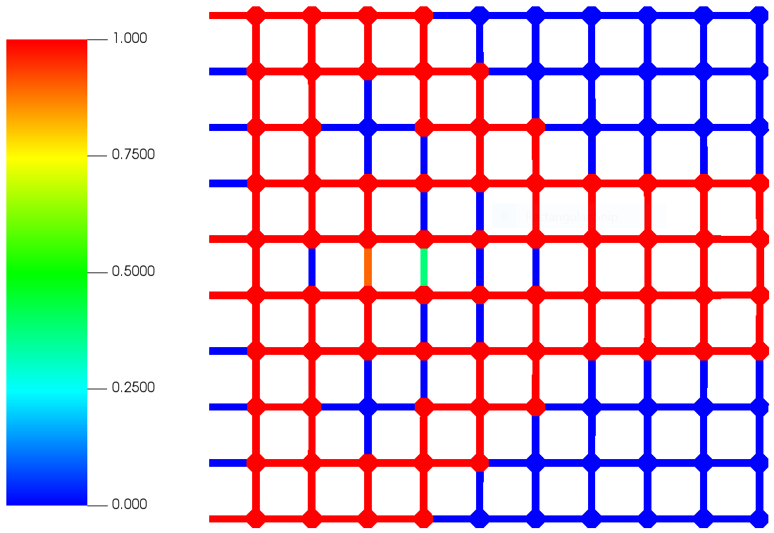

The SIMP penalization does not result in a purely black-and-white design; rather, there are a few components with intermediate values of . Therefore, post-processing is required to create a design that consists only of solid material and void regions. We choose to remove those components with , and set for the remaining components. The numerical results reported here are for a uniform initial condition for the optimizer. The initial value of compliance was Nm, the optimized value was Nm, and following post-processing the system by removing partially-void components, the obtained compliance value was still Nm to the fourth significant digit, and the result satisfies the volume fraction constraint. The configuration of the optimized system is shown in Fig. 7, with both the density field returned by the optimizer and the resulting structure. Random initialization does affect the final optimization result. For most choices of the random initialization (in which the optimization converges), there are several asymmetries in the parameter field; when beginning with a uniform initialization, the optimized structure is symmetrical. There is more than a single asymmetrical local optimum, as well. A few realizations of the random initial condition result in a final design that slightly improves on the compliance of the symmetrical design; however, the improvement is not retained after post-processing, because of components with intermediate densities that are removed. Instead, the final result is worse; therefore, we recommend using a uniform initial condition. Of course, this observation is mainly for MMA and for other optimization solvers, we may see different results.
6.2 A cantilever beam with a larger number of lattice components
The larger optimization example makes use of the same component discretizations and material properties as previously, but a lattice containing 2,950 components. This lattice is pictured in Fig. 8. The finite element mesh of the full system contains 9,362,520 nodes, for a total of 18,725,040 degrees of freedom in the system without static condensation. In this example, we compare the optimized solutions obtained from increasing resolution in the reduced order model; as in the comparison of performance for the forward model, we use port basis sizes of 4, 6, 8, 12, 16, and 20 basis functions. The total number of degrees of freedom in the CWROM then ranges from 16,080 to 80,400.
The system of components in this study form a cantilever beam with a homogeneous Dirichlet boundary condition on each of the ports on the left hand side of the domain. Two loads are placed on the system, on the right and bottom ports of the lowest right component. On the right port, a uniform pressure force of N/m to the right is added, while on the bottom port we impose a uniform pressure force of N/m downward.

The optimization is solved using the same optimization method and stopping criterion as the previous example; however, in this case we do not use a random initialization for multiple runs, but instead compare the solutions produced from a uniform initialization by different CWROM resolutions. In addition, we increase the stopping tolerance for change in the optimization parameter (Eq. (79)) to . The target mass fraction for this optimization was 25%. When post-processing, the tolerance for intermediate densities was increased, by removing only components with and setting for the rest; this results in a post-processed design that slightly exceeds the given upper bound for the mass fraction. Table 2 shows a comparison of the results obtained from different CWROM resolutions; the first column for compliance results is the value of the optimized compliance computed by the CWROM without post-processing, while the value in the final column is the value of the compliance computed by the highest-resolution CWROM using the post-processed densities. We also report the relative error for each discretization, measured against the solution of the CWFOM; the relative error is again given by Eq. (78). We note that the magnitude of the relative error is consistent with the results in the previous section, up until the basis size of 20; at very high resolutions of the CWROM, its solution matches the CWFOM more closely than it matched the full-order FEM model in the previous section. Some numerical error is still present. We only report optimization results up to a basis size of 20 here both due to the runtime of the optimization in our experimental implementation, and because, as shown below, the solution of the CWROM by a basis size of 20 is essentially the same as that of the CWFOM.
| Port dimension | Time (s) | (Nm) | (Nm) | Relative error |
|---|---|---|---|---|
| 4 | 38 | 8980.3 | 9051.5 | |
| 6 | 36 | 8989.5 | 8988.1 | |
| 8 | 101 | 8947.6 | 8882.5 | |
| 12 | 396 | 8951.6 | 8880.3 | |
| 16 | 558 | 9066.4 | 8965.5 | |
| 20 | 924 | 9066.3 | 8965.5 | |
| 36 | – | – | – |
A port basis size of 6 was faster than a port basis size of 4 due to faster convergence of the optimization; this trend did not continue for larger basis sizes. Up to a basis size of 12, the compliance of the optimized design after post-processing decreased, however, the two higher-dimensional CWROM’s actually resulted in a substantially worse design. This irregularity may indicate that the lower-dimensional CWROM smooths the objective function, allowing the the optimizer to find a lower local minimum than for higher basis sizes. There is a trade-off between time to solution and accuracy evident here; a basis size of 4 is probably not accurate enough for most purposes, as evidenced by the discrepancy between the compliance value returned by the optimizer and the significantly higher value resulting after post-processing. For a basis size of 6 or greater, however, the largest difference in compliance of the optimized designs is only approximately 1%, while the computational cost of the optimization increases rapidly.
We note that while the complexity estimates in Section 5 indicate that the runtime should increase quadratically with basis size, we actually observe a more rapid increase in practice, making the acceleration enabled by the CWROM even more significant.
In Fig. 9 and Fig. 10 we show the resulting density field and post-processed optimized structure obtained from the basis size 12 optimization (which resulted in the best design). The optimization was terminated based on the stopping criterion given in Eq. 79 after 153 iterations. The value of the compliance after optimization was 8,952 Nm, and post-processing did not remove any components with non-zero densities less than , and set the densities of 74 components with intermediate values of to 1. This resulted in a slightly lower compliance value in the post-processed structure, 8,880 Nm, at the cost of slightly exceeding the target mass fraction; the mass fraction of the post-processed structure is 25.3%.


In Fig. 11, we show the Von Mises stress field over a single component from the optimized system in 10. The resolved stress concentrations at the corners that are apparent in this plot illustrate a key benefit of the component-wise modeling approach for TO - it does not sacrifice high resolution solutions for the sake of speedup. In contrast with homogenization methods, which take the periodic structure to be at less than the length scale of a finite element, our approach allows computation of fields at the same length scale as the lattice structure. Approaches based on approximating lattice members as beam elements, on the other hand, solve an approximated form of the governing equation, while the CWROM solves the original problem in a reduced function space that nevertheless closely approximates the full FEM space as seen from the relative accuracies reported in Section 6.1.1.


7 Conclusion
We have demonstrated a component-wise topology optimization method that provides a combination of computational efficiency and accuracy not seen in other methods for lattice structure optimization. Using the static condensation formulation of Huynh et al. [46] and the port reduction of Eftang & Patera [33], we obtain a speedup in the solution of the forward model of over 1000x over a conforming FEM model, with relative error of less than 1%. We also show a key simplification of the component-wise method for the case where the parameter dependence of the linear elasticity weak form is linear in a function of parameter, providing further acceleration in our lattice structure design optimization using a SIMP parameterization. This work forms a base on which to build more sophisticated component-wise optimization frameworks; the high-resolution capability of the component-wise reduced order model is particularly intriguing in the context of stress-based TO. Future work will develop a stress-based component-wise formulation, and extend the SIMP parameterization used in this paper to include geometric parameters modifying the shape of members in the lattice structure.
Acknowledgments
This work was performed in part at Lawrence Livermore National Laboratory and was supported by the LDRD program fundings (i.e., 17-ER-026 and 20-FS-007). Lawrence Livermore National Laboratory is operated by Lawrence Livermore National Security, LLC, for the U.S. Department of Energy, National Nuclear Security Administration under Contract DE-AC52-07NA27344 and LLNL-JRNL-815816. This work was supported in part by the AEOLUS center under US Department of Energy Applied Mathematics MMICC award DE-SC0019303.
References
- [1] 3Dxpert. https://www.3dsystems.com/software/3dxpert. Accessed: 2020-07-13.
- [2] Ansys. http://www.ansys.com. Accessed: 2020-07-13.
- [3] AUTODESK WITHIN. http://www.withinlab.com/. Accessed: 2020-07-13.
- [4] COMSOL. https://www.comsol.com/. Accessed: 2020-07-13.
- [5] Meshify. http://www.adimant.com/meshify.html. Accessed: 2020-07-13.
- [6] nTopology. https://ntopology.com/. Accessed: 2020-07-13.
- [7] W Achtziger. Local stability of trusses in the context of topology optimization part i: exact modelling. Structural optimization, 17(4):235–246, 1999.
- [8] Wolfgang Achtziger, M Bendsøe, Aharon Ben-Tal, and Jochem Zowe. Equivalent displacement based formulations for maximum strength truss topology design. IMPACT of Computing in Science and Engineering, 4(4):315–345, 1992.
- [9] David Amsallem, Matthew Zahr, Youngsoo Choi, and Charbel Farhat. Design optimization using hyper-reduced-order models. Structural and Multidisciplinary Optimization, 51(4):919–940, 2015.
- [10] Erik Andreassen, Boyan S Lazarov, and Ole Sigmund. Design of manufacturable 3d extremal elastic microstructure. Mechanics of Materials, 69(1):1–10, 2014.
- [11] Harbir Antil, Matthias Heinkenschloss, Ronald HW Hoppe, Christopher Linsenmann, and Achim Wixforth. Reduced order modeling based shape optimization of surface acoustic wave driven microfluidic biochips. Mathematics and Computers in Simulation, 82(10):1986–2003, 2012.
- [12] J Ballani, DBP Huynh, DJ Knezevic, L Nguyen, and AT Patera. A component-based hybrid reduced basis/finite element method for solid mechanics with local nonlinearities. Computer Methods in Applied Mechanics and Engineering, 329:498–531, 2018.
- [13] Mervyn CC Bampton and Roy R Craig Jr. Coupling of substructures for dynamic analyses. Aiaa Journal, 6(7):1313–1319, 1968.
- [14] Martin P Bendsøe and Aharon Ben-Tal. Truss topology optimization by a displacements based optimality criterion approach. In Optimization of large structural systems, pages 139–155. Springer, 1993.
- [15] Martin P Bendsøe, Aharon Ben-Tal, and Jochem Zowe. Optimization methods for truss geometry and topology design. Structural optimization, 7(3):141–159, 1994.
- [16] Martin Philip Bendsoe and Noboru Kikuchi. Generating optimal topologies in structural design using a homogenization method. 1988.
- [17] M. P. Bendsøe. Optimal shape design as a material distribution problem. Structural optimization, 1(4):193–202, Dec 1989.
- [18] Paul T. Boggs and Jon W. Tolle. Sequential quadratic programming. Acta Numerica, 4:1–51, 1995.
- [19] Andreas Buhr, Christian Engwer, Mario Ohlberger, and Stephan Rave. Arbilomod, a simulation technique designed for arbitrary local modifications. SIAM Journal on Scientific Computing, 39(4):A1435–A1465, 2017.
- [20] Stefano Buoso, Andrea Manzoni, Hatem Alkadhi, André Plass, Alfio Quarteroni, and Vartan Kurtcuoglu. Reduced-order modeling of blood flow for noninvasive functional evaluation of coronary artery disease. Biomechanics and Modeling in Mechanobiology, 18(6):1867–1881, 2019.
- [21] Kevin Carlberg, Youngsoo Choi, and Syuzanna Sargsyan. Conservative model reduction for finite-volume models. Journal of Computational Physics, 371:280–314, 2018.
- [22] Wenjiong Chen, Xiaonan Zheng, and Shutian Liu. Finite-element-mesh based method for modeling and optimization of lattice structures for additive manufacturing. Materials, 11(11):2073, 2018.
- [23] Myung-Jin Choi, Myung-Hoon Oh, Bonyong Koo, and Seonho Cho. Optimal design of lattice structures for controllable extremal band gaps. Scientific reports, 9(1):1–13, 2019.
- [24] Youngsoo Choi, Gabriele Boncoraglio, Spenser Anderson, David Amsallem, and Charbel Farhat. Gradient-based constrained optimization using a database of linear reduced-order models. Journal of Computational Physics, page 109787, 2020.
- [25] Youngsoo Choi, Peter Brown, William Arrighi, Robert Anderson, and Kevin Huynh. Space–time reduced order model for large-scale linear dynamical systems with application to boltzmann transport problems. Journal of Computational Physics, page 109845, 2020.
- [26] Youngsoo Choi and Kevin Carlberg. Space–time least-squares petrov–galerkin projection for nonlinear model reduction. SIAM Journal on Scientific Computing, 41(1):A26–A58, 2019.
- [27] Youngsoo Choi, Deshawn Coombs, and Robert Anderson. Sns: a solution-based nonlinear subspace method for time-dependent model order reduction. SIAM Journal on Scientific Computing, 42(2):A1116–A1146, 2020.
- [28] Youngsoo Choi, Geoffrey Oxberry, Daniel White, and Trenton Kirchdoerfer. Accelerating design optimization using reduced order models. arXiv preprint arXiv:1909.11320, 2019.
- [29] Maxime Collet, Lise Noël, Matteo Bruggi, and Pierre Duysinx. Topology optimization for microstructural design under stress constraints. Structural and Multidisciplinary Optimization, 58(6):2677–2695, Dec 2018.
- [30] Niccolò Dal Santo, Simone Deparis, Andrea Manzoni, and Alfio Quarteroni. An algebraic least squares reduced basis method for the solution of nonaffinely parametrized stokes equations. Computer Methods in Applied Mechanics and Engineering, 344:186–208, 2019.
- [31] Gabriel Dimitriu, Ionel M Navon, and Răzvan Ştefănescu. Application of pod-deim approach for dimension reduction of a diffusive predator-prey system with allee effect. In International conference on large-scale scientific computing, pages 373–381. Springer, 2013.
- [32] W Dorn. Automatic design of optimal structures. J. de Mecanique, 3:25–52, 1964.
- [33] Jens L. Eftang and Anthony T. Patera. Port reduction in parametrized component static condensation: approximation and a posteriori error estimation. International Journal for Numerical Methods in Engineering, 96(5):269–302, 2013.
- [34] Jens L Eftang and Anthony T Patera. Port reduction in parametrized component static condensation: approximation and a posteriori error estimation. International Journal for Numerical Methods in Engineering, 96(5):269–302, 2013.
- [35] Anders Forsgren and Philip E. Gill. Primal-dual interior methods for nonconvex nonlinear programming. SIAM Journal on Optimization, 8(4):1132–1152, 1998.
- [36] Junjian Fu, Liang Xia, Liang Gao, Mi Xiao, and Hao Li. Topology optimization of periodic structures with substructuring. Journal of Mechanical Design, 141(7):071403, Jul 2019.
- [37] Mohamadreza Ghasemi and Eduardo Gildin. Localized model reduction in porous media flow. IFAC-PapersOnLine, 48(6):242–247, 2015.
- [38] Philip E. Gill, Walter Murray, and Michael A. Saunders. Snopt: An sqp algorithm for large-scale constrained optimization. SIAM Review, 47(1):99–131, 2005.
- [39] Sebastian Grimberg, Charbel Farhat, and Noah Youkilis. On the stability of projection-based model order reduction for convection-dominated laminar and turbulent flows. arXiv preprint arXiv:2001.10110, 2020.
- [40] Takao Hagishita and Makoto Ohsaki. Topology optimization of trusses by growing ground structure method. Structural and Multidisciplinary Optimization, 37(4):377–393, 2009.
- [41] Michael Hinze and Stefan Volkwein. Proper orthogonal decomposition surrogate models for nonlinear dynamical systems: Error estimates and suboptimal control. In Dimension reduction of large-scale systems, pages 261–306. Springer, 2005.
- [42] Chi Hoang, Youngsoo Choi, and Kevin Carlberg. arXiv preprint arXiv:2007.11835, 2020.
- [43] Harold Hotelling. Analysis of a complex of statistical variables into principal components. Journal of educational psychology, 24(6):417, 1933.
- [44] Walter C Hurty. Dynamic analysis of structural systems using component modes. AIAA journal, 3(4):678–685, 1965.
- [45] DBP Huynh. A static condensation reduced basis element approximation: Application to three-dimensional acoustic muffler analysis. International Journal of Computational Methods, 11(03):1343010, 2014.
- [46] Dinh Bao Phuong Huynh, David J Knezevic, and Anthony T Patera. A static condensation reduced basis element method: approximation and a posteriori error estimation. ESAIM: Mathematical Modelling and Numerical Analysis, 47(1):213–251, 2013.
- [47] Dinh Bao Phuong Huynh, David J Knezevic, and Anthony T Patera. A static condensation reduced basis element method: Complex problems. Computer Methods in Applied Mechanics and Engineering, 259:197–216, 2013.
- [48] Laura Iapichino, Alfio Quarteroni, and Gianluigi Rozza. Reduced basis method and domain decomposition for elliptic problems in networks and complex parametrized geometries. Computers & Mathematics with Applications, 71(1):408–430, Jan 2016.
- [49] Rui Jiang and Louis J Durlofsky. Implementation and detailed assessment of a gnat reduced-order model for subsurface flow simulation. Journal of Computational Physics, 379:192–213, 2019.
- [50] Steven G. Johnson. The nlopt nonlinear optimization package. http://github.com/stevengj/nlopt, 2008.
- [51] Sven Kaulmann, Mario Ohlberger, and Bernard Haasdonk. A new local reduced basis discontinuous galerkin approach for heterogeneous multiscale problems. 2011.
- [52] Youngkyu Kim, Youngsoo Choi, David Widemann, and Tarek Zohdi. A fast and accurate physics-informed neural network reduced order model with shallow masked autoencoder. arXiv preprint arXiv:2009.11990, 2020.
- [53] Uri Kirsch. Fundamental properties of optimal topologies. In Topology Design of Structures, pages 3–18. Springer, 1993.
- [54] Hyeong Seok Koh, Jun Hwan Kim, and Gil Ho Yoon. Efficient topology optimization of multicomponent structure using substructuring-based model order reduction method. Computers & Structures, 228:106146, Feb 2020.
- [55] A Kolmogoroff. Uber die beste annaherung von funktionen einer gegebenen funktionenklasse. Annals of Mathematics, pages 107–110, 1936.
- [56] Karl Kunisch and Stefan Volkwein. Galerkin proper orthogonal decomposition methods for a general equation in fluid dynamics. SIAM Journal on Numerical analysis, 40(2):492–515, 2002.
- [57] Michel Loeve. Probability Theory. D. Van Nostrand, New York, 1955.
- [58] Siavash Haroun Mahdavi and Sean Hanna. An evolutionary approach to microstructure optimisation of stereolithographic models. In The 2003 Congress on Evolutionary Computation, 2003. CEC’03., volume 1, pages 723–730. IEEE, 2003.
- [59] Kristo Mela. Resolving issues with member buckling in truss topology optimization using a mixed variable approach. Structural and Multidisciplinary Optimization, 50(6):1037–1049, 2014.
- [60] M Mordhorst, Timm Strecker, D Wirtz, Thomas Heidlauf, and Oliver Röhrle. Pod-deim reduction of computational emg models. Journal of Computational Science, 19:86–96, 2017.
- [61] Max M. Opgenoord and Karen E. Willcox. Aeroelastic tailoring using additively manufactured lattice structures. In 2018 Multidisciplinary Analysis and Optimization Conference. American Institute of Aeronautics and Astronautics, Jun 2018.
- [62] Cosmin G. Petra. A memory-distributed quasi-newton solver for nonlinear programming problems with a small number of general constraints. Journal of Parallel and Distributed Computing, 2018.
- [63] Kathrin Smetana. A new certification framework for the port reduced static condensation reduced basis element method. Computer Methods in Applied Mechanics and Engineering, 283:352–383, 2015.
- [64] Kathrin Smetana and Anthony T Patera. Optimal local approximation spaces for component-based static condensation procedures. SIAM Journal on Scientific Computing, 38(5):A3318–A3356, 2016.
- [65] R Ştefănescu and Ionel Michael Navon. Pod/deim nonlinear model order reduction of an adi implicit shallow water equations model. Journal of Computational Physics, 237:95–114, 2013.
- [66] Mathias Stolpe. Truss optimization with discrete design variables: a critical review. Structural and Multidisciplinary Optimization, 53(2):349–374, 2016.
- [67] Krister Svanberg. The method of moving asymptotes: a new method for structural optimization. International Journal for Numerical Methods in Engineering, 24(2):359–373, 1987.
- [68] Sylvain Vallaghé, Phuong Huynh, David J Knezevic, Loi Nguyen, and Anthony T Patera. Component-based reduced basis for parametrized symmetric eigenproblems. Advanced Modeling and Simulation in Engineering Sciences, 2(1):7, 2015.
- [69] Andreas Wächter and Lorenz T. Biegler. On the implementation of an interior-point filter line-search algorithm for large-scale nonlinear programming. Mathematical Programming, 106(1):25–57, 2006.
- [70] Chuang Wang, Ji Hong Zhu, Wei Hong Zhang, Shao Ying Li, and Jie Kong. Concurrent topology optimization design of structures and non-uniform parameterized lattice microstructures. Structural and Multidisciplinary Optimization, 58(1):35–50, 2018.
- [71] Yaguang Wang and Zhan Kang. Concurrent two-scale topological design of multiple unit cells and structure using combined velocity field level set and density model. Computer Methods in Applied Mechanics and Engineering, 347:340–364, Apr 2019.
- [72] Yingjun Wang, Hang Xu, and Damiano Pasini. Multiscale isogeometric topology optimization for lattice materials. Computer Methods in Applied Mechanics and Engineering, 316:568–585, Apr 2017.
- [73] Seth Watts, William Arrighi, Jun Kudo, Daniel A Tortorelli, and Daniel A White. Simple, accurate surrogate models of the elastic response of three-dimensional open truss micro-architectures with applications to multiscale topology design. Structural and Multidisciplinary Optimization, 60(5):1887–1920, 2019.
- [74] Daniel A White, William J Arrighi, Jun Kudo, and Seth E Watts. Multiscale topology optimization using neural network surrogate models. Computer Methods in Applied Mechanics and Engineering, 346:1118–1135, 2019.
- [75] Zijun Wu, Liang Xia, Shuting Wang, and Tielin Shi. Topology optimization of hierarchical lattice structures with substructuring. Computer Methods in Applied Mechanics and Engineering, 345:602–617, 2019.
- [76] Huanhuan Yang and Alessandro Veneziani. Efficient estimation of cardiac conductivities via pod-deim model order reduction. Applied Numerical Mathematics, 115:180–199, 2017.
- [77] Yanfang Yang, Mohammadreza Ghasemi, Eduardo Gildin, Yalchin Efendiev, Victor Calo, et al. Fast multiscale reservoir simulations with pod-deim model reduction. SPE Journal, 21(06):2–141, 2016.
- [78] Huikai Zhang, Yaguang Wang, and Zhan Kang. Topology optimization for concurrent design of layer-wise graded lattice materials and structures. International Journal of Engineering Science, 138:26–49, May 2019.
- [79] Pengfei Zhao, Cai Liu, and Xuan Feng. Pod-deim based model order reduction for the spherical shallow water equations with turkel-zwas finite difference discretization. Journal of Applied Mathematics, 2014, 2014.