Holographic insulator/superconductor phase transitions with excited states

Introducing a variable $z=r_{s}/r$ for convenience, we can rewrite Eqs. (3) and (4) into

where the function $f$ is $f(z)=(1-z^{4})/z^{2}$ and the prime denotes the derivative with respect to $z$.

It has been shown numerically in the previous section that, for both the ground and excited states of the s-wave holographic dual model in the backgrounds of AdS soliton, there is a phase transition between the insulator and superconductor phases around the critical chemical potential $\mu_{c}$. Since the scalar field $\psi$ vanishes as long as one approaches the critical point $\mu_{c}$ from below, we can get a general solution to Eq. (28) at the critical point

with an integration constant $c_{1}$. According to the Neumann-like boundary condition for the gauge field $\phi$, we have to set $c_{1}=0$ to keep $A_{t}$ finite at the tip $z=1$. Thus, for the case of $\mu\leq\mu_{c}$, we obtain the physical solution $\phi(z)=\mu$ to Eq. (28).

In order to match the behavior of $\psi$ at the boundary (5), we define a trial function $F(z)$ which satisfies

with $i=+/-$. Here we have imposed the boundary condition $F(0)=1$. With the help of Eq. (27) and the physical solution $\phi(z)$ in Eq. (29), we find

with

According to the Sturm-Liouville eigenvalue approach Gelfand-Fomin, the eigenvalue $q\mu/r_{s}$ can be achieved from the extremal values of the following function by virtue of the Rayleigh Quotient

Before proceeding, we would like to make a comment. In order to derive the expression (33), we have employed the boundary condition $[T(z)F(z)F^{\prime}(z)]|_{0}^{1}=0$. Note that $T(1)\equiv 0$ from Eq. (32), so the condition $T(1)F(1)F^{\prime}(1)=0$ is satisfied automatically. However, for the case of $m^{2}=-15/4$ considered here, the condition $T(0)F(0)F^{\prime}(0)=0$ is not satisfied automatically for the operator $\mathcal{O}_{-}$ since the leading order contribution from $T(z)$ as $z\rightarrow 0$ is $2\Delta_{-}-3=0$ but is satisfied automatically for the operator $\mathcal{O}_{+}$ since $2\Delta_{+}-3=2>0$. Thus, we have to impose the Neumann boundary condition $F^{\prime}(0)=0$ for the operator $\mathcal{O}_{-}$, just as analyzed in Refs. QiaoEHS; LvPLB2020; HFLi; WangSPJ.

As an example, we calculate the case for the operator $\mathcal{O}_{-}$ by using the fourth order trial function

which satisfies the Neumann boundary condition $F^{\prime}(0)=0$ with three constants $a_{2}$, $a_{3}$ and $a_{4}$. From Eq. (18), we have

which gives us the dimensionless critical chemical potential $q\mu_{c}/r_{s}$ and corresponding value of $a_{k}$ from the ground state to the third excited state by computing the extremal values of the above expression, i.e., $q\mu_{c}^{(0)}/r_{s}=0.836$ at $a_{2}=0.384$, $a_{3}=-0.157$ and $a_{4}=-0.002$, $q\mu_{c}^{(1)}/r_{s}=3.053$ at $a_{2}=5.298$, $a_{3}=-2.998$ and $a_{4}=0.231$, $q\mu_{c}^{(2)}/r_{s}=5.432$ at $a_{2}=20.306$, $a_{3}=-30.120$ and $a_{4}=8.793$, and $q\mu_{c}^{(3)}/r_{s}=7.847$ at $a_{2}=47.655$, $a_{3}=-120.749$ and $a_{4}=76.511$. Comparing with the analytical results from the second order trial function in HFLi, we can obtain the first four lowest-lying modes by using the fourth order trial function $F(z)$.

In order to investigate the higher excited states of the s-wave holographic insulator/superconductor phase transition by using the analytical Sturm-Liouville method, we include the eighth order of $z$ in the trial function $F(z)$, i.e., $F(z)=1-\sum_{k=2}^{k=8}a_{k}z^{k}$ for the operator $\mathcal{O}_{-}$, and $F(z)=1-\sum_{k=1}^{k=8}a_{k}z^{k}$ for the operator $\mathcal{O}_{+}$ in the following calculation, where $a_{k}$ is a constant. Using the expression (33) to compute the extremal values, we can get the critical chemical potentials from the ground state to the sixth excited state, which have been presented in Tables 2 and 3. Compared with the numerical results shown in Table 1, the agreement of the analytical results and numerical calculation is impressive, which implies that the Sturm-Liouville method is powerful to study the s-wave holographic insulator/superconductor phase transition even if we consider the excited states.

From Tables 2 and 3, we confirm analytically that for both operators the critical chemical potential $\mu_{c}$ increases as the number of nodes $n$ increases, which supports the numerical observation obtained in Table 1 that an excited state has a higher critical chemical potential than the corresponding ground state. Fitting the relation between $q\mu_{c}/r_{s}$ and $n$ by using the analytical results, we get

which is in good agreement with the numerical fitting results given in Eq. (II.1). This can be used to back up the numerical computation that, for both operators $\mathcal{O}_{-}$ and $\mathcal{O}_{+}$, the difference of the dimensionless critical chemical potential $q\mu_{c}/r_{s}$ between the consecutive states is about 2.4.

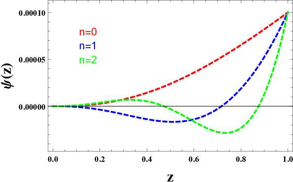
On the other hand, for the scalar field mass $m^{2}=-15/4$, in Fig. 4 we use the expression (30) to give the distribution of the scalar field $\psi(z)$ as a function of $z$ for the scalar operators $\mathcal{O}_{-}$ and $\mathcal{O}_{+}$ by setting the initial condition $\psi(1)=0.0001$, which agrees well with the numerical calculation shown in Fig. 1. Interestingly enough, besides the critical chemical potential, the Sturm-Liouville method with the higher order of $z$ in the trial function $F(z)$ can also study the behaviors of the scalar field near the critical point of the phase transition.

Since the condensate of the scalar operator $\langle{\cal O}_{i}\rangle$ is so small near the critical point, we can expand $\phi(z)$ in terms of small $\langle{\cal O}_{i}\rangle$ by

which leads to the equation of motion for $\chi(z)$

where we have defined a new function $W(z)=zf(z)$ and introduced the boundary condition $\chi(1)=0$ at the tip.

Considering the asymptotic behavior of $\phi$ in Eq. (5), we expand $\phi$ when $z\rightarrow 0$ as

Comparing the coefficients of the $z^{0}$ term in both sides of the above formula, we can easily get

where $\chi(0)=c_{2}-\int_{0}^{1}W^{-1}[c_{3}+\int_{1}^{z}x^{2\Delta_{i}-3}F(x)^{2}dx]dz$ with the integration constants $c_{2}$ and $c_{3}$ which can be determined by the boundary condition of $\chi(z)$ in Eq. (41). For example, in the case of $m^{2}=-15/4$ considered here, for the operator $\mathcal{O}_{-}$ we find that

which agrees well with the numerical result given in Eq. (II.1). Here the critical chemical potentials $\mu^{(0)}_{c}$, $\mu^{(1)}_{c}$ and $\mu^{(2)}_{c}$, which correspond to the ground, first and second excited states, are given in Table 2. Obviously, the expression (43) is valid for all cases considered here. Therefore, it is shown clearly that, for both operators $\mathcal{O}_{-}$ and $\mathcal{O}_{+}$, the phase transition between the s-wave insulator and superconductor is second order and the condensate approaches zero as $\langle{\cal O}_{i}\rangle\sim\left(\mu-\mu^{(n)}_{c}\right)^{\beta}$ with the mean-field critical exponent $\beta=1/2$ for all the states.

From the coefficients of the $z^{1}$ term in Eq. (42), we note that $\chi^{\prime}(0)\rightarrow 0$, which is consistent with the following relation by making integration of both sides of Eq. (41)

Moving to the coefficients of the $z^{2}$ term in Eq. (42), we obtain

with $\Gamma(m,n)=[2\chi(0)]^{-1}\int_{0}^{1}z^{2\Delta_{i}-3}F^{2}dz$, which is a function of the scalar field mass $m^{2}$ and the number of nodes $n$. As an example, we observe that for the operator $\mathcal{O}_{-}$ with the fixed mass $m^{2}=-15/4$

which again can be compared with the numerical result presented in Eq. (II.1), where the critical chemical potentials $\mu^{(0)}_{c}$, $\mu^{(1)}_{c}$ and $\mu^{(2)}_{c}$ are given in Table 2, corresponding to the ground, first and second excited states, respectively. Thus, we point out that, in the vicinity of the transition point, one may find a linear relationship between the charge density and chemical potential, namely, $\rho\sim\left(\mu-\mu^{(n)}_{c}\right)$ in the present model for all the states, which is in agreement with the numerical calculation shown previously in Eqs. (II.1) and (II.1) for both operators $\mathcal{O}_{-}$ and $\mathcal{O}_{+}$.

Changing the coordinate from $r$ to $z$ by $z=r_{s}/r$, we can express Eqs. (55) and (56) in the $z$ coordinate as

with the function $f(z)=(1-z^{4})/z^{2}$. Here and hereafter in this section the prime denotes the derivative with respect to $z$.

Considering the vector field $\rho_{x}=0$ at the critical chemical potential $\mu_{c}$ for the the ground and excited states, just as shown in Figs. 6 and 7, we can obtain the physical solution $A_{t}(z)=\mu$ to Eq. (80) when $\mu<\mu_{c}$, which takes the same form as that in the s-wave holographic insulator/superconductor model. Thus, assuming that $\rho_{x}$ takes the form

with the boundary condition $F(0)=1$ satisfying the boundary behavior of $\rho_{x}$ in (57), we get the equation of motion for the trial function $F(z)$

with

where $V(z)$ has been introduced in (32). Following the standard procedure for the Sturm-Liouville eigenvalue problem Gelfand-Fomin, we can deduce the eigenvalues of $q\mu/r_{s}$ from variation of the following function

Since $Q(1)\equiv 0$ and $Q(0)\equiv 0$ for the case of $\Delta=1+\sqrt{1+m^{2}}$ with the mass beyond the Breitenlohner-Freedman (BF) bound $m^{2}_{BF}=-1$ Breitenloher, just as discussed in Sec. II for the s-wave holographic insulator/superconductor phase transition with the excited states, the condition $[Q(z)F(z)F^{\prime}(z)]|_{0}^{1}=0$ can be satisfied automatically for the vector operator $\mathcal{O}_{x}$. This means that we shall require $F(z)$ to satisfy the Dirichlet boundary condition $F(0)=1$ rather than the Neumann boundary condition $F^{\prime}(0)=0$. Thus, we expand the trial function $F(z)$ up to the eighth order, i.e., $F(z)=1-\sum_{k=1}^{k=8}a_{k}z^{k}$ for the operator $\mathcal{O}_{x}$ in the following calculation.