Hyperbolicity of Augmented Links in the Thickened Torus

Alice Kwon and Ying Hong Tham

Abstract.

For a hyperbolic link $K$ in the thickened torus, we show there is a decomposition of the complement of a link $L$ , obtained from augmenting $K$ , into torihedra. We further decompose the torihedra into angled pyramids and finally angled tetrahedra. These fit into an angled structure on a triangulation of the link complement, and thus by [5], this shows that $L$ is hyperbolic.

1. Introduction

Given a twist-reduced diagram of a link $K$ , augmenting is a process in which an unknotted circle component (augmentation) is added to one or more twist regions (a single crossing or a maximal string of bigons) of $K$ . The newly obtained link is called an augmented link and the newly obtained diagram is called an augmented link diagram. See Figure 2.

Adams showed in [2] that given a hyperbolic alternating link $K$ in ${S}^{3}$ the link $L$ obtained by augmenting $K$ is hyperbolic. In this paper we investigate if this statement holds for links in the thickened torus i.e. if $L$ is a link obtained from augmenting a hyperbolic alternating link $K$ in the thickened torus. We define augmenting similarly for links in the thickened torus with their associated link diagram on ${\mathbb{T}^{2}}\times\{0\}.$

Menasco [9] showed that there are decompositions of the complements of alternating links in ${S}^{3}$ into two topological polyhedra, a top polyhedron and a bottom polyhedron. For alternating links $K$ in the thickened torus, Champanerkar, Kofman and Purcell [4] showed that there is a decomposition of the complement of $K$ into objects called torihedra, which we think of as counterparts to Menasco’s decomposition for links in the thickened torus; just like Menasco’s decomposition, one obtains a top and a bottom torihedron.

In Section 2 we show that for augmented links in the thickened torus (not necessarily fully augmented), one can also obtain a decomposition of the complement into a top and bottom torihedron. In Section 3, we prove that many augmented alternating links in the thickened torus are hyperbolic.

We point out that in [7], the first author proved that fully augmented links in the thickened torus are hyperbolic, so this paper can be seen as a generalization of that work.

While revising this paper, we learned that [1] proves a generalization of our work here, showing hyperbolicity of generalized augmented links in an arbitrary thickened surface. We note that our approach, based on angle structures, is different from theirs, which is based on topological arguments.

Refer to caption — Figure 1. (a) pretzel knot before augmentation (b) pretzel knot after augmentation; second diagram shows removal of full twists in the augmented twist regions.

2. Augmented Links

We denote $I=(-1,1)$ .

Champanerkar, Kofman and Purcell have studied alternating links in the thickened torus [4]. They define a link in the thickened torus as a quotient of a biperiodic alternating link as follows:

Definition 2.1.

A biperiodic alternating link ${\mathcal{L}}$ is an infinite link in $\mathbb{R}^{2}\times I$ with a link diagram ${\mathcal{D}}\subset\mathbb{R}^{2}$ such that ${\mathcal{L}}$ and ${\mathcal{D}}$ are invariant under the action of a two dimensional lattice $\Lambda$ on $\mathbb{R}^{2}$ by translations.

The quotient $L=\mathcal{L}/\Lambda$ is an alternating link in the thickened torus ${\mathbb{T}^{2}}\times I$ , whose projection onto ${\mathbb{T}^{2}}\times\{0\}=\mathbb{R}^{2}\times\{0\}/\Lambda$ is an alternating link diagram ${\mathcal{D}}/\Lambda$ .

We refer to ${\mathbb{T}^{2}}\times\{0\}$ as the projection plane.

Remark 2.2.

Since ${\mathbb{T}^{2}}\times I\cong{S}^{3}-H$ , where $H$ is a Hopf link. The complement ${\mathbb{T}^{2}}\times I-L={S}^{3}-(L\cup H)$ .

Champanerkar, Kofman and Purcell [4] extended the definition of prime links in ${S}^{3}$ for links in ${\mathbb{T}^{2}}\times I$ called weakly prime.

Definition 2.3.

A diagram $D\subset{\mathbb{T}^{2}}$ of a link $L$ in the thickened torus ${\mathbb{T}^{2}}\times I$ is weakly prime if whenever a disk is embedded in ${\mathbb{T}^{2}}$ meets the diagram transversely in exactly two edges, then the disk contains a simple edge of the diagram and no crossings.

Definition 2.4.

Recall that a twist region in a link diagram in the plane is a maximal sequence of vertices such that consecutive vertices are two vertices of a bigon face, and consecutive bigons meet at exactly one vertex. The length of the twist region is the number of bigons.

We say a single vertex $v$ is a trivial twist region (or twist region of length 0) if, for some cyclical ordering $f_{1},f_{2},f_{3},f_{4}$ of the four faces adjacent to $v$ , $f_{1},f_{3}$ are not bigons. Note that if all four faces are not bigons, then we think of $v$ as being a trivial twist region in two ways, and in this sense, every vertex is part of exactly two twist regions.

For links in the thickened torus, a twist region in a link diagram of $L=\mathcal{L}/\Lambda$ in ${\mathbb{T}^{2}}\times I$ , is the quotient of a twist region in the biperiodic link $\mathcal{L}$ .

Definition 2.5.

A biperiodic link $\mathcal{L}$ is called twist-reduced if for any simple closed curve on the plane that intersects the diagram of $\mathcal{L}$ transversely in four points, with two points adjacent to one crossing and the other two points adjacent to another crossing, the simple closed curve bounds a subdiagram consisting of a collection of bigons strung end to end between these crossings. We say the diagram of $L$ is twist-reduced if it is the quotient of a twist-reduced biperiodic link diagram.

Now we can define augmentation for a link in ${\mathbb{T}^{2}}\times I$ the same way we define augmentation for links in ${S}^{3}$ :

Definition 2.6.

Let $D(K)$ be a twist-reduced diagram of a link $K$ in ${\mathbb{T}^{2}}\times I$ . We define augmenting as a process in which an unknotted circle component, called a crossing circle, is added to one or more twist regions of $D(K)$ (see Figure 2); we call the resulting link $L$ an augmented link obtained from $K$ . We say $L$ is fully augmented if $L$ is obtained by augmenting $K$ at every crossing/twist region.

As pointed out in the introduction, after augmenting a twist region, a standard Dehn twist argument allows us to remove a full twist (that is, two bigons).

Definition 2.7.

We say an augmentation has a half twist if at least one of the augmented twist regions has an odd number of vertices (i.e. even number of bigons).

Definition 2.8.

A graph $G=(V,E)$ on the torus is cellular if its complement is a collection of open disks.

We note that when a link diagram is cellular, a twist region in the torus cannot be a cycle; otherwise, the face adjacent to the twist region would have non-trivial homology.

2.1. Torihedral Decomposition of Augmented Alternating Links in Thickened Torus

We present a method of decomposing an augmented link (not necessarily fully augmented) in the thickened torus into objects called “torihedra” as defined below. Decomposing alternating links in the thickened torus into torihedra were first described in [4], then later used for fully augmented links in the thickened torus in [7]. The idea is to combine methods of Menasco [9] and the use of crossing edges at each crossing of our link and Lackenby’s “cut-slice-flatten” method [8] on the augmentation sites.

Definition 2.9.

[4] A torihedron ${\mathcal{T}}$ is a cone on the torus, i.e. ${\mathbb{T}^{2}}\times[0,1]/({\mathbb{T}^{2}}\times\{1\})$ , with a cellular graph $G=G({\mathcal{T}})$ on ${\mathbb{T}^{2}}\times\{0\}$ . The ideal torihedron ${\mathcal{T}}^{\circ}$ is ${\mathcal{T}}$ with the vertices of $G$ and the vertex ${\mathbb{T}^{2}}\times\{1\}$ removed. Hence, an ideal torihedron is homeomorphic to ${\mathbb{T}^{2}}\times[0,1)$ with a finite set of points (ideal vertices) removed from ${\mathbb{T}^{2}}\times\{0\}$ . We refer to the vertex ${\mathbb{T}^{2}}\times\{1\}$ as the cone point of ${\mathcal{T}}$ .

For visualization purposes, we typically draw the graph $G({\mathcal{T}})$ of a torihedron from the perspective of the cone point ${\mathbb{T}^{2}}\times\{1\}$ . Note however that later we will be dealing with “top” and “bottom” torihedra that are glued together along their torus boundary faces; to avoid confusion, we will visualize the graphs of both torihedra from the perspective of the cone point of the “top” torihedron.

Since the faces of $G({\mathcal{T}})$ are disks, ${\mathcal{T}}$ can be decomposed into a union of pyramids, where each pyramid is obtained by coning a face of $G({\mathcal{T}})$ to the cone point of ${\mathcal{T}}$ . This also gives a decomposition of the corresponding ideal torihedron ${\mathcal{T}}^{\circ}$ into ideal pyramids. We call these the pyramidal decompositions of ${\mathcal{T}}$ and ${\mathcal{T}}^{\circ}$ .

Definition 2.10.

Let $G$ be a graph on the torus. Let $v$ be a vertex and $e,e^{\prime}$ be distinct edges that meet $v$ . A bow-tie modification to $v,e,e^{\prime}$ is the process of removing $v,e,e^{\prime}$ and adding in a pair of triangular faces, which we refer to as bow-tie faces or a bow-tie (see Figure 3, 4). The edges of the bow-tie are of three types; diagonal edges, which do not touch $v$ , long edges, which are “parallel” to the original edges $e,e^{\prime}$ , and short edges. A bow-tie modification is a left bow-tie modification if, traveling from $v$ out along $e$ and $e^{\prime}$ , the diagonal faces appear to the left of $e$ and $e^{\prime}$ , respectively; likewise for right bow-tie modifications.

Figure 3. Bow-tie modifications and its relation to torihedra

Figure 4. Another example of (left) bow-tie modification

Definition 2.11.

We say a twist region is right-augmented if, when both strands are (locally) oriented so that they cross the augmentation disk in the same direction, the crossing is a right-handed half-twist. We say a twist is left-augmented if it is not right-augmented. (See Figure 3).

In other words, we have the tautological-sounding fact that augmenting a right-handed twist region is a right-handed augmentation.

We can recover $L$ from the link diagram of $K$ together with labels at twist regions indicating left- or right-augmentation.

Definition 2.12.

Let $L$ be a link obtained from augmenting an alternating link $K$ with a cellular link diagram $D=D(K)$ . We define the top/bottom bow-tie graph of $L$ as follows. (See Figure 5 for illustrations.)

Let $D^{\prime}$ be the graph obtained from $D$ by collapsing each augmented twist region of $K$ to a vertex. Clearly, $D^{\prime}$ is the link diagram of a link $K^{\prime}$ obtained from $K$ by removing half-twists from each augmented twist region until one crossing remains. Let $v_{t}$ denote a vertex of $D^{\prime}$ corresponding to an augmented twist region of $K$ , and let $v_{c}$ denote a vertex of $D^{\prime}$ corresponding to a crossing of $K$ not in an augmented twist region.

Orient the edges of $D^{\prime}$ to point from an undercrossing to an overcrossing. Label the two outgoing edges at vertex $v$ (which corresponds to a crossing or a twist region) by $e_{v}^{(1)},e_{v}^{(2)}$ (in arbitrary order). For each left- (resp. right-) augmented twist region $t$ , we perform a left (resp. right) bow-tie modification to $v_{t},e_{v_{t}}^{(1)},e_{v_{t}}^{(2)}$ .

We call the resulting graph the top bow-tie graph of $L$ , denoted by $\Gamma_{T}(L)$ . If we had oriented the edges of $D^{\prime}$ the other way, and subsequently performed the same operations, we obtain another graph, which we call the bottom bow-tie graph of $L$ , denoted by $\Gamma_{B}(L)$ .

Note that the non-bow-tie faces of $\Gamma_{T}(L)$ and $\Gamma_{B}(L)$ are naturally identified with the faces of $D^{\prime}$ (as the bow-tie modification procedure does not remove faces).

Figure 5. Constructing the top and bottom bow-tie graphs, using bow-tie modifications

Proposition 2.13.

Let $K$ be an alternating link in the thickened torus with a cellular link diagram, and let $L$ be an augmented link obtained from $K$ . There is a decomposition of the complement, $({\mathbb{T}^{2}}\times I)-L$ , into two ideal torihedra.

Moreover, the graphs of the torihedra are the top and bottom bow-tie graphs from Definition 2.12, $\Gamma_{T}(L)$ and $\Gamma_{B}(L)$ , respectively.

We call this the torihedral decomposition of the link complement of $L$ in the thickened torus.

Proof.

As mentioned before, we will be combining Menasco’s method using crossing edges at each crossing and Lackenby’s “cut-slice-flatten” method on augmentation sites.

Let $L=K\cup C$ , with $C$ being the collection of crossing circles. Arrange $L$ in the following way: place the circle components in $C$ perpendicular to the projection plane ${\mathbb{T}^{2}}\times\{0\}$ , and leave the remaining part of the link $K\subseteq L$ lying in the projection plane (except at crossings of $K$ ). Thus, the projection of $L$ onto the projection plane will be a diagram $D(K)$ of $K$ together with line segments corresponding to crossing circles.

We now place a crossing edge at each crossing of $K$ , connecting the top and bottom strands at the crossing (see Figure 6). We also three horizontal edges for each crossing circle (see Figure 7, leftmost diagram).

Figure 6. Splitting and flattening crossing edges.

View the link from the point at infinity from the top end ( ${\mathbb{T}^{2}}\times\{1\}$ ) of the thickened torus. At each crossing of $K$ , push the top strand towards the bottom strand, splitting the crossing edge into two identical edges and spreading them apart as in Figure 6. Note that after this operation, the link (which is no longer a link) for both top and bottom look the same, but a crossing edge associated to a crossing is pushed in different directions; this contributes to a “ $2\pi/n$ twist” when gluing back the faces of the top and bottom torihedra.

Now for each crossing circle $c$ , consider a spanning (twice-punctured) disk $B_{c}$ . The following operations are depicted in Figure 7. $B_{c}$ intersects the projection plane ${\mathbb{T}^{2}}\times\{0\}$ , cutting $B_{c}$ into two pieces $B_{c}^{+},B_{c}^{-}$ , each being an ideal triangle. We then slice along the disk $B_{c}$ , turning it into two copies, $B_{c}^{(1)},B_{c}^{(2)}$ (in no particular order); each copy $B_{c}^{(j)}$ is also cut horizontally into two pieces, $B_{c}^{(j),+},B_{c}^{(j),-}$ . We untwist all crossings in the twist region which $c$ encircles, rotating $B_{c}^{(j)}$ by $180^{\circ}$ for each crossing. Then we flatten the disks; the crossing circle is shrunk to a point, as it is at infinity.

Figure 7. Cut-slice-flatten; the even and odd refer to the number of crossings in that twist region (we only draw one crossing in the first diagram); the top and bottom graphs are glued back, gray face to gray face, white face to white face; note that the graph does not depend on the parity of the number of crossings, but the gluing is different

Finally, we shrink all remaining segments of the link $L$ to ideal vertices. It is easy to see that the top and bottom graphs are exactly $\Gamma_{T}(L)$ and $\Gamma_{B}(L)$ from Definition 2.12. To recover the link complement, we glue bow-tie to bow-tie as described in Figure 7, and glue each non-bow-tie face to its natural counterpart (see Definition 2.12), with a “ $2\pi/n$ ” twist as discussed before.

∎

The Figures 8 to 11 depict an example which decomposes the link (C) of Figure 2.

Remark 2.14.

We note that our main Theorem 3.4 requires that all non-trivial twist regions be augmented, but Proposition 2.13 does not require it.

Definition 2.15.

An angled torihedron $({\mathcal{T}},\theta_{\bullet}^{*})$ is a torihedron ${\mathcal{T}}$ with an assignment of an interior dihedral angle $\theta_{e}^{*}\in[0,\pi]$ to each edge $e$ of $G({\mathcal{T}})$ such that for each vertex $v\in G({\mathcal{T}})$ , $\sum_{e\ni v}\theta_{e}^{*}=(\deg(v)-2)\pi$ . We also denote $\theta_{e}=\pi-\theta_{e}^{*}$ , so $\sum_{e\ni v}\theta_{e}=2\pi$ ; we refer to $\theta_{e}$ as the exterior dihedral angle. For brevity, we write dihedral angle to mean interior dihedral angle.

We say $({\mathcal{T}},\theta_{\bullet}^{*})$ is degenerate if $\theta_{e}^{*}=0$ for some edge; we say it is non-degenerate otherwise.

One may ask for the pyramidal decomposition of a torihedron to “respect” angles. The following definitions, in particular an “angle splitting”, make sense of this.

Definition 2.16.

An angled ideal tetrahedron is an ideal tetrahedron with an assignment of an interior dihedral angle $\theta_{e}^{*}$ to each edge $e$ , such that

•

each dihedral angle is in $[0,\pi]$ ;
•

for each tetrahedron, opposite edges have equal dihedral angles;
•

the three distinct interior angles at edges incident to one vertex sum to $\pi$ .

We say an angled ideal tetrahedron is degenerate if one dihedral angle is 0; we say it is non-degenerate otherwise.

Definition 2.17.

A base-angled ideal pyramid is a pyramid whose base is an $n$ -gon, $n\geq 3$ , and each boundary edge $e_{i}$ of the base face is assigned a dihedral angle $\alpha_{i}\geq 0$ such that their sum is $\sum\alpha_{i}=\pi$ . The vertical edge $e_{i}^{\prime}$ that meets $e_{i}$ and $e_{i+1}$ is automatically assigned the dihedral angle $\pi-\alpha_{i}-\alpha_{i+1}$ .

We say a base-angled ideal pyramid is degenerate if $\alpha_{i}=0$ for some $i$ ; we say it is non-degenerate otherwise.

Clearly, the dihedral angles of an ideal hyperbolic pyramid make it a base-angled ideal pyramid (with $\alpha_{i}=\varphi_{e_{i}}$ ); it is not hard to see that the converse is true: simply consider a circumscribed polygon such that the side $e_{i}$ subtends an angle of $2\alpha_{i}$ at the center, and take the ideal hyperbolic pyramid over it in upper-half space. Also, an angled ideal tetrahedron is simply a base-angled ideal pyramid with base a triangle, and with no preferred face.

Definition 2.18.

An angle-splitting of an angled torihedron $({\mathcal{T}},\theta_{\bullet}^{*})$ is an assignment of an angle $\varphi_{\vec{e}}$ to each oriented edge $\vec{e}$ , such that

•

for each edge $e$ , $\theta_{e}^{*}=\varphi_{\vec{e}}+\varphi_{\overset{\leftarrow}{e}}$ , where $\overset{\leftarrow}{e}$ is the opposite orientation on $e$ ,
•

for each face $f$ , $\sum_{\vec{e}\in\partial f}\varphi_{\vec{e}}=\pi$ , where $\vec{e}\in\partial f$ is the edge in the boundary of $f$ taken with outward-orientation (see Convention 2.19).

Equivalently, an angle-splitting is a decomposition of ${\mathcal{T}}$ into base-angled pyramids, one for each face $F$ of $G({\mathcal{T}})$ , such that the interior dihedral of the edge $\vec{e}\in\partial F$ is $\varphi_{\vec{e}}$ .

We also say that $\varphi_{\bullet}$ is an angle-splitting of the edge-labeled graph $(G({\mathcal{T}}),\theta_{\bullet}^{*})$ .

We say that an angle-splitting is degenerate if $\varphi_{\vec{e}}=0$ for some oriented edge $\vec{e}$ ; it is non-degenerate otherwise.

Convention 2.19.

The outward-orientation on the boundary of a face is the orientation such that the face is to the left of the boundary. An assignment/label on an oriented edge $\vec{e}$ (for example, $\varphi_{\vec{e}}$ ) will usually be drawn to the left of that edge.

Remark 2.20.

These $\theta$ ’s are the same as the $\theta$ ’s in [3], and angle-splittings $\varphi_{\bullet}$ ’s are the same as their “coherent angle system”.

Lemma 2.21.

Let $P_{n}$ be a base-angled ideal pyramid, and suppose we are given a decomposition of the base face into triangles by adding new edges. One gets an obvious corresponding triangulation of $P_{n}$ , where a new face is added for each new edge. Then there is an assignment of a dihedral angle to each edge of each ideal tetrahedron in this triangulation such that

•

each tetrahedron is an angled ideal tetrahedron;
•

the sum of dihedral angles around each new edge is $\pi$ ;
•

the dihedral angles of the edges of the original base face are the same as before.

Moreover, if $P_{n}$ is non-degenerate, then the resulting angled tetrahedra are also non-degenerate.

Proof.

Induct on $n$ ; there is nothing to prove for the base case $n=3$ .

The proof is essentially given in Figure 12. We spell it out here in words.

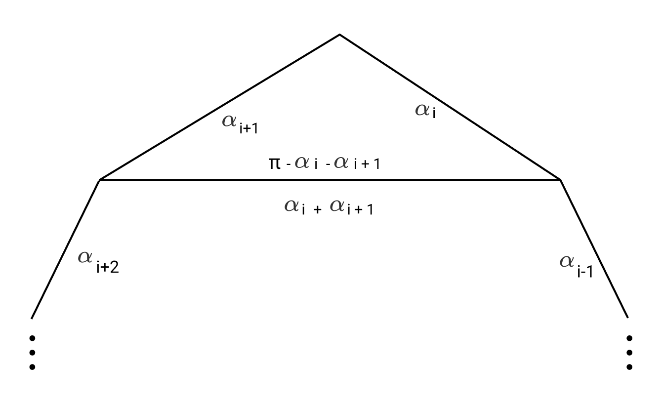
Suppose the edges are labeled $e_{i}$ , for an edge which goes between vertices $v_{i}$ and $v_{i+1}$ , and suppose $e_{i}$ is assigned dihedral angle $\alpha_{i}$ . Let $e^{\prime}$ be a new edge added to the base face of $P_{n}$ such that it separates the base face into a triangle and an $(n-1)$ -gon; suppose the sides of the triangle are $e_{i},e_{i+1}$ , and $e^{\prime}$ . The new face corresponding to $e^{\prime}$ separates $P_{n}$ into an ideal tetrahedron $T$ and an ideal pyramid $P_{n-1}$ . We assign the dihedral angle of $\pi-\alpha_{i}-\alpha_{i+1}$ to $e^{\prime}$ in $T$ , and assign $\alpha_{i}+\alpha_{i+1}$ to $e^{\prime}$ in $P_{n-1}$ . Clearly the sum of dihedral angles condition is satisfied in $T$ and $P_{n-1}$ . It remains to check that the dihedral angles assigned to the vertical (non-base) edges are correct. For the vertical edge associated to $v_{j}$ for $j\neq i,i+2$ , there is nothing to check; for $j=i$ , the dihedral angles are $\pi-\alpha_{i}-(\pi-\alpha_{i}-\alpha_{i-1})$ in $T$ and $\pi-\alpha_{i-1}-(\alpha_{i}+\alpha_{i+1})$ in $P_{n-1}$ , which sum to $\pi-\alpha_{i}-\alpha_{i+1}$ ; it is similar for $j=i+2$ .

Non-degeneracy of the resulting angled tetrahedra follows easily from the observation that the angles assigned to each side of a new edge is simply the sum of the angles of original edges on the other side. ∎

3. Hyperbolicity of Augmented Links

Thurston introduced a method for finding the unique complete hyperbolic metric for a given 3-manifold $M$ with boundary consisting of tori [10]. Thurston wrote down a system of gluing and consistency equations which can be translated to equations involving angles for a triangulation of $M$ whose solutions correspond to the complete hyperbolic metric on the interior of $M$ . Casson and Rivin separated Thurston’s gluing equations into a linear and non-linear part [5]. Angle structures are solutions to the linear part of Thurston’s gluing equations. By Theorem 3.2 ([6, Theorem 1.1]), to prove hyperbolicity of a link complement, it suffices to find an angle structure on a triangulation of the link complement.

Definition 3.1.

Let $M$ be an orientable 3-manifold with boundary consisting of tori. An angle structure on an ideal triangulation $\tau$ of $M$ is an assignment of a dihedral angle to each edge of each tetrahedron, such that

•

each tetrahedron is a non-degenerate angled ideal tetrahedron,
•

around each edge of $\tau$ , the dihedral angles sum to $2\pi$ .

Theorem 3.2.

[6, Theorem 1.1] Let $M$ be a 3-manifold with a triangulation that admits an angle structure. Then $M$ is hyperbolic.

For a hyperbolic link $K$ in ${\mathbb{T}^{2}}\times I$ , we show that the link $L$ obtained from augmenting $K$ is hyperbolic. The idea is to start with a graph from the torihedral decomposition of the link $K$ which will give us a graph on each torihedron with an angle assignment of $\pi/2$ to each edge [4]. By Proposition 2.13, there is a torihedral decomposition of the complement of the augmented link $L$ . Using those angles from $K$ , we then assign new angles locally to edges of torihedra from a torihedral decomposition of $L$ and decompose them into base-angled pyramids which can be decomposed into tetrahedra, thus obtaining an angle structure on a triangulation.

We need the following theorem, adapted from [3, Theorem 4], specialized to genus 1 surfaces:

Theorem 3.3.

[3, Theorem 4] Let $\Gamma=(V,E)$ be a graph on the torus, and let $\check{\Gamma}=(F,\check{E})$ be the dual graph, with $\check{E}$ being naturally identified with $E$ . Let $f\in(0,\pi)^{E}$ be a function on the set of edges $E$ that sums to $2\pi$ around each vertex of $V$ ; let $f^{*}(e)=\pi-f(e)$ .

There exists a non-degenerate angle-splitting of $(\Gamma,f^{*})$ if and only if the following is satisfied:

Suppose we cut the torus along a subset of edges in the dual graph $\check{\Gamma}$ , obtaining one or more pieces; Then for any piece that is a disk, the sum of $f$ over the edges in the boundary of the piece is at least $2\pi$ , with equality if and only if the piece contains exactly one vertex of $\Gamma$ .

The original theorem [3, Theorem 4] proves that a circle pattern combinatorially equivalent to $\Gamma$ exists; a circle pattern naturally yields an angle-splitting (which they call a coherent angle system).

Theorem 3.4.

Let $K$ be a weakly prime, alternating link in the thickened torus whose diagram is cellular and has no bigons. Let $L$ be a link obtained from augmenting $K$ . Then $L$ is hyperbolic.

More generally, if $K$ is as above with a twist-reduced diagram containing bigons, and $L$ is obtained by augmenting $K$ such that for every twist region with at least one bigon is augmented, then $L$ is hyperbolic.

Proof.

By Proposition 2.13, ${{\mathbb{T}^{2}}\times I-L}$ can be obtained by gluing two torihedra ${\mathcal{T}}_{T}(L),{\mathcal{T}}_{B}(L)$ with graphs $\Gamma_{T}(L),\Gamma_{B}(L)$ .

Recall that $\Gamma_{T}(L),\Gamma_{B}(L)$ are obtained by bow-tie modifications of the diagram $D^{\prime}$ of a link $K^{\prime}$ (see Definition 2.12). Assign to each edge $e$ of $D^{\prime}$ the angle $\theta_{e}=\pi/2$ (so that $\theta_{e}^{*}=\pi/2$ too). This assignment has the property that the sum of dihedral angles around each identified edge (in the complement of $K^{\prime}$ ) is $2\pi$ . This can be achieved because of the hypotheses on bigons in our theorem statement.

Using the fact that $K^{\prime}$ is weakly prime (which easily follows from $K$ being weakly prime), it is not hard to see that the condition on cocycles of Theorem 3.3 is satisfied by this assignment. Thus, there exists a non-degenerate angle-splitting $\varphi_{\bullet}$ of $(D^{\prime},\theta_{\bullet}^{*})$ .

Now we perform the bow-tie modifications to obtain $\Gamma_{T}(L),\Gamma_{B}(L)$ . For each step (i.e. each bow-tie modification), we show how to modify the $\theta^{*}$ assignments and how to get angle-splittings. Say we perform such a modification at some vertex $v$ and two edges $e^{(1)},e^{(2)}$ . We assign new $\theta_{\bullet}^{*}$ angles to the resulting bow-tie modification graph as in Figure 13. Note that the sum of $\theta$ (not $\theta^{*}$ ) around each vertex is still $2\pi$ . Figure 14 shows an angle-splitting of this assignment.

We check that upon gluing the top and bottom torihedra, the sum of interior dihedral angles $\theta^{*}$ around each edge is $2\pi$ : crossing edges have $\theta^{*}=\pi/2$ , and appear four times, twice in each torihedron, while for bow-tie edges, simply check for half-twist and non-half-twist cases separately.

Now we have a decomposition of the two torihedra into degenerate base-angled pyramids (recall that that means some of the interior dihedral angles $\theta^{*}$ are 0); since we need the pyramids to be non-degenerate, we modify the graph on the torihedra and the angle assignments to make all $\theta^{*}$ non-zero as follows.

We first modify the graphs on the torihedra by adding edges to them for some extra “flexibility”. Consider a face $f$ of $\Gamma_{T}(L)$ that is not from a bow-tie. Suppose the corresponding face $\bar{f}$ of $D^{\prime}$ had vertices $v_{1},\ldots,v_{n}$ in counter-clockwise order. Note that $f$ may meet a vertex twice, but we label each occurrence with its own index. We label the edges of $f$ by $e_{i,0}$ , $e_{i,\pi}$ , or $e_{i}$ , depending on whether the $\theta^{*}$ of that edge is $0$ , $\pi$ , or $\pi/2$ respectively. More precisely, for a vertex $v_{i}$ corresponding to a crossing of $K$ that is not augmented, we label $e_{v_{i}}^{(.)}$ by $e_{i}$ (here $e_{v_{i}}^{(.)}$ is $e_{v_{i}}^{(1)}$ or $e_{v_{i}}^{(2)}$ , whichever meets $\bar{f}$ ; see Definition 2.12). For a vertex $v_{i}$ that corresponds to a twist region of $K$ , if the crossing circle “faces” $f$ , then $f$ meets a diagonal edge of the bow-tie corresponding to $v_{i}$ , and we label it $e_{i}$ (for example if $f$ is the top left face in Figure 14 (a)); if not, then $f$ meets a short and long edge of the corresponding bow-tie, and we label them by $e_{i,0}$ and $e_{i,\pi}$ , respectively (for example if $f$ is the top right face in Figure 14 (b)).

If $\bar{f}$ does not have vertices of the latter kind, i.e. if $f$ does not meet short or long edges, then we will not modify $f$ . So assume that $\bar{f}$ does have such a vertex, and suppose it is right-augmented (the other case is treated similarly). Then for all right-augmented vertices $v_{i}$ of $\bar{f}$ , $f$ would meet the short, long edges $e_{i,0},e_{i,\pi}$ , while for all left-augmented vertices, $f$ would meet the diagonal edges. In particular, the edges $e_{i,0},e_{i,\pi}$ always appear in counter-clockwise order.

Suppose, after cyclically reindexing, $v_{1},\ldots,v_{k}$ is a maximally contiguous subsequence of right-augmented vertices of $D^{\prime}$ around $\bar{f}$ ; the edges around $f$ would start $e_{1,0},\linebreak e_{1,\pi},\linebreak e_{2,0},\linebreak e_{2,\pi},\linebreak\ldots,\linebreak e_{k,0},\linebreak e_{k,\pi},\linebreak\ldots$ . We add new edges across $f$ as follows (see Figure 15; ignore the + and - signs for now):

•

Case $k=n$ : (i.e. every vertex of $\bar{f}$ is right-augmented.) In this case, we do nothing.
•

Case: There is only one such maximal contiguous subsequence:
- –
  
  Subcase: $k=1$ : We add an edge that goes across $e_{1,0},e_{1,\pi},e_{2}$ (in the sense that the new edge separates the edges of $f$ into two sets, one of them being those three edges; since $n\geq 3$ , this edge is new).
- –
  
  Subcase: $k\geq 2$ : We add an edge across $e_{1,0},e_{1,\pi}$ and another edge across $e_{2,0},e_{2,\pi},e_{3,0},\ldots,e_{k,\pi}$ (these two edges do not form a bigon because we’ve ruled out $k=n$ ).
•

Case: There are multiple such maximal contiguous subsequences. We just add edges as in the previous case for each contiguous subsequence, except one special case: when the edges of $f$ are exactly $e_{1,0},e_{1,\pi},e_{2},e_{3,0},e_{3,\pi},e_{4}$ , we add only one edge separating the first three edges from the other three. (This prevents formation of a bigon.)

Figure 15. Adding edges to non-bow-tie faces; the

+,-

labels are short for

+1,-1

respectively.

This way we obtain a new graph $\Gamma_{T}^{\prime}$ , which defines a new torihedron ${\mathcal{T}}_{T}^{\prime}$ . We make ${\mathcal{T}}_{T}^{\prime}$ angled using the angles from ${\mathcal{T}}_{T}(L)$ for old edges, and putting $\theta^{*}=\pi$ for all new edges.

We can get an angle-splitting for $(\Gamma_{T}^{\prime},\theta^{*})$ , using the angle-splitting for $\Gamma_{T}(L)$ for old edges, and for a new edge $e$ (as in Figure 15) that cuts through some face $f$ of $\Gamma_{T}(L)$ , we assign $\varphi_{\vec{e}}=\sum\varphi_{\vec{e^{\prime}}}$ , where the sum is over all the edges $\vec{e^{\prime}}\in\partial f$ on the other side of $\vec{e}$ . By non-degeneracy of the angle-splitting on $D^{\prime}$ , these assignments to the new edges are all non-zero.

Now fix some small $\varepsilon>0$ . Let $\varphi_{\vec{e}}^{\prime}=\varphi_{\vec{e}}+x\cdot\varepsilon$ , where $x$ is the label (in Figure 15) on $\vec{e}$ (set $x=0$ if unlabeled). Let $\theta_{e}^{\prime*}=\varphi_{\vec{e}}^{\prime}+\varphi_{\overset{\leftarrow}{e}}^{\prime}$ . It is easy to check that the sum of labels around each vertex is 0, hence $\theta^{\prime*}$ defines an angled torihedron $({\mathcal{T}}_{T}^{\prime},\theta^{\prime*})$ . For each face of $\Gamma_{T}^{\prime}$ , the $+/-$ labels on the inner side of boundary edges cancel out: for bow-tie faces, the short edge gets a $+1$ and the long edge gets $-1$ , while for non-bow-tie faces, it is clear from Figure 15. Hence, $\varphi^{\prime}$ is an angle-splitting of $({\mathcal{T}}_{T}^{\prime},\theta^{\prime*})$ . Furthermore, all shorts edges (which are the only edges with $\varphi_{\vec{e}}=0$ ) have a $+1$ label on each side, so $\varphi^{\prime}$ is non-degenerate.

Now we perform the same operations for the bottom torihedron, adding new edges to $\Gamma_{B}(L)$ to get $\Gamma_{B}^{\prime}$ in the same manner; note that left and right augmentations are switched, so that the order of $e_{i,0},e_{i,\pi}$ are switched. Thus all the $+/-$ labels in Figure 15 should have switched signs. We also get a nondegenerate angle-splitting $\varphi^{\prime}$ of an angled torihedron $({\mathcal{T}}_{B}^{\prime},\theta^{\prime*})$ .

By construction, under the gluing of ${\mathcal{T}}_{T}(L)$ to ${\mathcal{T}}_{B}(L)$ , the new edges added to $\Gamma_{T}(L)$ are glued to the new edges added to $\Gamma_{B}(L)$ , since they are added by the same procedure. As noted before, upon gluing ${\mathcal{T}}_{T}(L)$ to ${\mathcal{T}}_{B}(L)$ the sum of exterior dihedral angles $\theta^{*}$ around each edge is $2\pi$ . This clearly remains true after adding the new edges (they’re labeled $\pi$ on each torihedron). Again by construction, the $+/-$ labels coming from the top and bottom diagrams get canceled out. Thus, upon gluing ${\mathcal{T}}_{T}^{\prime}$ to ${\mathcal{T}}_{B}^{\prime}$ , the sum of new exterior dihedral angles $\theta^{\prime*}$ around each edge is still $2\pi$ .

Finally, we obtain a triangulation with an angle structure as follows. For each face of $\Gamma_{T}^{\prime}$ that has more than three sides, we arbitrarily decompose it into triangles and apply Lemma 2.21 to obtain a triangulation of ${\mathcal{T}}_{T}^{\prime}$ into non-degenerate angled tetrahedra; perform the corresponding decomposition for faces of $\Gamma_{B}^{\prime}$ and obtain a triangulation of ${\mathcal{T}}_{B}^{\prime}$ into non-degenerate angled tetrahedra. These triangulations glue up into a triangulation of ${{\mathbb{T}^{2}}\times I-L}$ with an angle structure. Thus, by Theorem 3.2, $L$ is hyperbolic. ∎

Remark 3.5.

By applying Theorem 3.4 judiciously, one may prove hyperbolicity of augmented links that do not satisfy its hypotheses as stated.

Say we have a link $K$ that satisfies the stricter hypotheses of Theorem 3.4 (no bigons). Consider a crossing circle $C$ around two parallel strands that do not meet at a crossing. The addition of $C$ to $K$ is not an augmentation as in Definition 2.6, and so Theorem 3.4 does not directly apply. However, we may consider the related link $K^{\prime\prime}$ where those two strands have a full twist, so that the addition of $C$ to $K^{\prime\prime}$ is an augmentation. Now Theorem 3.4 applies to $K^{\prime\prime}\cup C$ , and thus $K\cup C$ is also hyperbolic.

Note that augmenting in the sense of Definition 2.6 will not turn a non-weakly prime link into a weakly prime link, but the above extended notion of augmenting might.

Another way to squeeze more out of Theorem 3.4 is to consider augmenting twist regions in the “transverse direction”. That is, suppose $K$ has only one twist region $T$ , which is left-handed, but we perform a right-handed augmentation at each vertex of $T$ (instead of a single left-handed augmentation, which is required for Theorem 3.4). Consider the link $K^{\prime\prime}$ where each vertex of $T$ is replaced by a right-handed twist region of length 2 (two bigons). Then the twist region $T$ “is” no longer a twist region in $K^{\prime\prime}$ , and we may freely apply Theorem 3.4) and conclude that the “transversely augmented” $K$ is hyperbolic.

References

[1] Colin Adams, Michele Capovilla-Searle, Darin Li, Qiao Li, Jacob McErlean, Alexander Simons, Natalie Stewart, and Xiwen Wang. Generalized augmented cellular alternating links in thickened surfaces are hyperbolic. arXiv preprint arXiv:2107.05406, 2021.
[2] Colin C. Adams. Augmented alternating link complements are hyperbolic. In Low-dimensional topology and Kleinian groups (Coventry/Durham, 1984), volume 112 of London Math. Soc. Lecture Note Ser., pages 115–130. Cambridge Univ. Press, Cambridge, 1986.
[3] Alexander I. Bobenko and Boris A. Springborn. Variational principles for circle patterns and Koebe’s theorem. Trans. Amer. Math. Soc., 356(2):659–689, 2004.
[4] Abhijit Champanerkar, Ilya Kofman, and Jessica S. Purcell. Geometry of biperiodic alternating links. J. Lond. Math. Soc. (2), 99(3):807–830, 2019.
[5] David Futer and François Guéritaud. From angled triangulations to hyperbolic structures. In Interactions between hyperbolic geometry, quantum topology and number theory, volume 541 of Contemp. Math., pages 159–182. Amer. Math. Soc., Providence, RI, 2011.
[6] David Futer and François Guéritaud. From angled triangulations to hyperbolic structures. In Interactions between hyperbolic geometry, quantum topology and number theory, volume 541 of Contemp. Math., pages 159–182. Amer. Math. Soc., Providence, RI, 2011.
[7] Alice Kwon. Fully augmented links in the thickened torus. arXiv preprint arXiv:2007.12773, 2020.
[8] Marc Lackenby. The volume of hyperbolic alternating link complements. Proc. London Math. Soc. (3), 88(1):204–224, 2004. With an appendix by Ian Agol and Dylan Thurston.
[9] William W. Menasco. Polyhedra representation of link complements. In Low-dimensional topology (San Francisco, Calif., 1981), volume 20 of Contemp. Math., pages 305–325. Amer. Math. Soc., Providence, RI, 1983.
[10] W. P. Thurston. The geometry and topology of three-manifolds. Princeton Univ. Math. Dept. Notes. Available at http://www.msri.org/communications/books/gt3m. [2, 21, 50, 58, 68, 87, 89, 94, 97, 99, 138, 196], 1979.


(a)	(b)


(a)	(b)