Turbulent relaxation to equilibrium in a two-dimensional quantum vortex gas
Abstract
We experimentally study emergence of microcanonical equilibrium states in the turbulent relaxation dynamics of a two-dimensional chiral vortex gas. Same-sign vortices are injected into a quasi-two-dimensional disk-shaped atomic Bose-Einstein condensate using a range of mechanical stirring protocols. The resulting long-time vortex distributions are found to be in excellent agreement with the mean-field Poisson-Boltzmann equation for the system describing the microcanonical ensemble at fixed energy and angular momentum . The equilibrium states are characterized by the corresponding thermodynamic variables of inverse temperature and rotation frequency . We are able to realize equilibria spanning the full phase diagram of the vortex gas, including on-axis states near zero-temperature, infinite temperature, and negative absolute temperatures. At sufficiently high energies the system exhibits a symmetry-breaking transition, resulting in an off-axis equilibrium phase at negative absolute temperature that no longer shares the symmetry of the container. We introduce a point-vortex model with phenomenological damping and noise that is able to quantitatively reproduce the equilibration dynamics.
I Introduction
Turbulence continues to stand as one of the most challenging problems in physics despite several centuries of study. Most phenomena occurring in the turbulent motion of fluids are strongly nonequilibrium in nature, making the problem highly intractable for theoretical treatment. The chaotic fluid motion ultimately requires a probabilistic description, yet one of the most powerful probabalistic tools available — the maximum entropy principle of statistical mechanics — is effectively rendered useless; turbulent flows generally defy a description in terms of equilibrium statistical mechanics, due to their strong dissipation of energy and consequent lack of detailed balance Thalabard et al. 2015; Frisch 1995; Batchelor 1953.
A notable exception occurs in the case of quasi-two-dimensional flows, where, due to the suppression of vortex stretching, energy is conserved in the limit of large Reynolds number Kraichnan 1967; Batchelor 1969. In such flows, large and long-lived isolated vortices tend to spontaneously form out of the turbulent background. Examples are regularly seen in a range of systems including electron plasmas Sarid et al. 2004a; Rodgers et al. 2009, soap films Kellay 2017, stratified fluid layers Hansen et al. 1998, and planetary atmospheres Adriani et al. 2018; Bouchet and Sommeria 2002 — Jupiter’s Great Red Spot, which has persisted for over 350 years, is perhaps the most famous example. The prevalence and long-lived nature of these structures suggests they are an aspect of turbulence to which equilibrium statistical mechanics could be successfully applied.
The idea to apply statistical mechanics to turbulent flows originated with the seminal work Onsager Onsager 1949, who investigated the statistical mechanics of a system of point vortices in a perfect (i.e., inviscid) fluid. In this simple Hamiltonian model, the vortices are treated as a kind of “gas”, whose particles interact via long-range interactions. The equilibria of this model are indeed typically dominated by one or two large clusters of vortices, reflecting what is typical of real fluids. While the point-vortex approach could not be quantitatively applied to real fluids (which have continuous vorticity distributions), Onsager’s maximum entropy approach was, naturally, a highly appealing prospect; a significant body of work in the following decades aimed to bridge the gap between the discrete and continuous vorticity distributions Joyce and Montgomery 1973; Edwards and Taylor 1974; Kraichnan 1975; Miller 1990; Robert 1991; Robert and Sommeria 1991, in the hope to connect the maximum entropy approach to real fluids (for a summary of theoretical developments, see, e.g., Maestrini and Salman 2019).
Unfortunately however, although equilibrium theories have proven to be successful in some cases Denoix 1992; Matthaeus et al. 1991; Rodgers et al. 2009; Bouchet and Sommeria 2002, they also fail in many situations. It has been argued that “statistical approaches have not been proven yet to offer a more than qualitative framework for the interpretation of experimental observation” Tabeling 2002. Some examples explicitly avoid assuming global entropy maximization Sarid et al. 2004b, while others require abandoning entropy altogether Driscoll and Fine 1990; Carnevale et al. 1992; Marteau et al. 1995; Huang and Driscoll 1994; Pakter and Levin 2018. One major culprit, it seems, is the ergodicity assumption; two-dimensional turbulent systems often do not exhibit sufficiently vigorous (ergodic) mixing to justify the search for global equilibrium states Tabeling 2002. Indeed, it is now known that a general property of long-range interacting systems is that they are unable to thermalize when they contain a large number of degrees of freedom Levin et al. 2014 — precisely the situation which occurs in large Reynolds number flows Batchelor 1953; Batchelor 1969. A second major complication arises due to contributions in the boundary layer, which introduces crucial changes to the flow near the container walls for any nonvanishing value of viscocity Brands et al. 1999; Li and Montgomery 1996; Van Heijst et al. 2006.
Superfluid atomic gases confined in uniform box traps Gaunt et al. 2013; Chomaz et al. 2015; Gauthier et al. 2016; Mukherjee et al. 2017; Tajik et al. 2019; Navon et al. 2021 have recently emerged as a new platform to test fundamental theories of turbulence and vortex dynamics in a highly tunable system Navon et al. 2016; Navon et al. 2019; Glidden et al. 2021; Gauthier et al. 2019a; Johnstone et al. 2019; Stockdale et al. 2020; Kwon et al. 2021. A natural question which arises is whether the maximum entropy approach may more accurately describe coherent vortices in a superfluid, due to several advantages these systems offer. First, in superfluids the viscosity is identically zero, as is assumed in the maximum entropy theories discussed above. Second, in thin-layer superfluids the vorticity is genuinely pointlike in nature, and the condensate wave function constrains the vorticity to be quantized with value , where is Planck’s constant and is the mass of a superfluid particle. In fact, provided the vortex cores are small, the vortex dynamics are governed precisely by the Hamiltonian point-vortex system originally considered by Onsager Fetter 1966; Groszek et al. 2018. These systems therefore offer the unique prospect of experimentally testing the maximum entropy approach in a system which is genuinely inviscid, and contains a relatively small number of degrees of freedom (determined by the vortex number, ), where simulations suggest that the ergodicity assumption may hold Dritschel et al. 2015; Esler and Ashbee 2015; Salman and Maestrini 2016. Significant experimental progress in this direction has been made in two recent works Gauthier et al. 2019a; Johnstone et al. 2019 (one by some of the present authors Gauthier et al. 2019a), which observe signatures consistent with maximum entropy vortex distributions. However, these experiments both suffer from key limitations: (i) The temperature of the vortex distributions could only be inferred from a priori assumptions of equilibrium, and (ii) the relaxation to equilibrium is not tested for a wide range of nonequilibrium initial conditions. Without having tested these aspects it cannot yet be said whether the maximum entropy approach proves useful for describing two-dimensional turbulent flows in superfluids.
In this work we demonstrate that the maximum entropy approach quantitatively agrees with experiment over a wide range of parameters. We experimentally consider a chiral (single-sign circulation) vortex gas confined to a disk geometry, which we realize in an ultracold atomic Bose-Einstein condensate confined with a fully configurable optical potential. In contrast to the previous experiments Gauthier et al. 2019a; Johnstone et al. 2019 which consider neutral vortex gas systems Joyce and Montgomery 1973; Yu et al. 2016, the chiral system exhibits nontrivial (i.e., spatially nonuniform) equilibria over the entire the phase diagram Smith 1989, facilitating a comparison between experiment and theory over the full phase diagram of the vortex gas. Furthermore, as all vortices have the same sign, vortex-antivortex annihilation is completely suppressed in the bulk of the superfluid. By suppressing this nonequilibrium process, the interpretation of the system in terms of the microcanonical ensemble is simplified considerably.
Using controllable optical potentials to stir the superfluid, we are able to initialize vortex distributions of – vortices with essentially arbitrary initial values of energy and angular momentum, which are the two control parameters determining the equilibrium states. We find that, despite some residual dissipation, the vortex gas lives long enough to reach equilibrium. We first initialize the system directly into a near-equilibrium state, and demonstrate that it remains near equilibrium, undergoing a gradual cooling. Then, by initializing the vortices in nonequilibrium configurations with different energy and angular momenta, we demonstrate relaxation to a range of equilibrium distributions predicted by the microcanonical ensemble. Finally, we introduce a point-vortex model with damping and noise that is able to quantitatively reproduce the equilibration dynamics.
The outline of this paper is as follows. In Sec. II we outline the point-vortex system and summarize the known results from statistical mechanics and the mean-field phase diagram of the chiral vortex gas. In Sec. III we present our experimental results and compare the observed vorticity distributions with the equilibrium predictions presented in Sec. II. Our results on the dynamics of the vortex gas are presented in Sec. IV, which we show can be quantitatively described by a point-vortex model supplemented by friction and noise. Section V presents conclusions and outlook.

II Chiral vortex gas in a disk
Before presenting our experimental results, we first provide context by briefly introducing the model of a chiral vortex gas in a disk, and we review the known equilibrium results obtained from statistical mechanics.
II.1 point-vortex model
We consider a two-dimensional fluid containing a chiral vortex gas of point vortices with quantized circulations , where is Planck’s constant and is the mass of a fluid particle. The fluid is assumed to be incompressible and inviscid, with a uniform (areal) density , and is confined to a disk of radius . Hereafter we may set without loss of generality. In addition to the vortex number , the kinetic energy and angular momentum of the fluid are conserved. The kinetic energy of the fluid can be expressed in terms of the vortex locations as Newton 2013; Smith and O’Neil 1990
| (1) |
Here is expressed in units of the energy . Notice that, although the energy is entirely kinetic, the Hamiltonian resembles the interaction energy in a “gas” of charged particles in two dimensions; the first term describes the Coulomb-like interaction between vortices, while second term describes the interaction between vortices and image vortices, which have circulation and are located outside the disk at position where . The fictitious image vortices enforce the condition that the fluid may not flow through the boundary, i.e., , where is the radial unit vector. The vortex dynamics governed by are given by
| (2) |
It can be seen from Eq. (2) that the and coordinates of the vortices are canonically conjugate variables. This unusual feature of this Hamiltonian system has a profound effect on the statistical mechanics, as will be discussed in the next section. The angular momentum is , where
| (3) |
The angular momentum hence constrains the mean-square radius of the vortex distribution 11 1 is often referred to as the angular momentum Newton 2013; Aref 1979. The distinction is not so important when applying the point-vortex model to the dynamics of a classical Euler fluid (where the vortex number is conserved), but is for a superfluid as vortex annihilation can occur at the boundary; here varies continuously as a vortex leaves at the boundary, whereas changes discontinuously..
II.2 Statistical mechanics
For the Hamiltonian system described by Eq. (1), at sufficiently large one may hope to invoke the ergodicity hypothesis to determine the long-time behavior of the system from the tools of statistical mechanics. For the vortex gas dynamically evolving at fixed energy [Eq. (1)] and angular momentum [Eq. (3)], the system is described by the microcanonical ensemble
| (4) |
where is the entropy, and
| (5) |
Here is the inverse temperature and is a thermodynamic potential for the angular momentum. The quantity may be interpreted as a rotation frequency 22 2 Note however that for a given solution does not necessarily correspond to any particular physical rotation rate in the system; see Ref. Smith and O’Neil 1990..
A remarkable property of Eqs. (1) and (2) is that the canonical coordinates are determined only by the circulations and the physical-space coordinates of the vortices. As first appreciated by Onsager Onsager 1949, this property has profound effects on the statistical mechanics of the system; if the physical space is bounded by a container of area , it follows that the total accessible phase space volume is bounded:
| (6) |
It follows directly from this property Onsager 1949 that entropy reaches a maximum at a finite value of the energy [see Fig. 1(a), point B]. Above this energy, the entropy decreases with increasing energy, and by Eq. (5) these equilibria are thus characterized by negative absolute temperatures. The bounded phase space property starkly contrasts with most systems, for which the phase space is unbounded and the entropy monotonically increases with energy. Notice crucially that the unusual Hamiltonian structure occurs because the vortices are massless objects; there is no term in the Hamiltonian of the form (for hypothetical vortex mass ). The appearance of such a term would break the bounded phase space condition Eq. (6). Finally, it should be noted that as this system supports negative temperatures, ensemble equivalence does not hold in general, and the canonical ensemble is therefore not appropriate Levin et al. 2014; Smith and O’Neil 1990.
| Solution | A: Rankine | B: Gaussian | C: Riccati | D: off-Axis | E: supercondensate |
|---|---|---|---|---|---|
| Density |
![[Uncaptioned image]](2010.10049v3/rankine.png)
|
![[Uncaptioned image]](2010.10049v3/gaussian.png)
|
![[Uncaptioned image]](2010.10049v3/riccati.png)
|
![[Uncaptioned image]](2010.10049v3/offaxis.png)
|
![[Uncaptioned image]](2010.10049v3/supercondensate.png)
|
| — | -2 | ||||
| 0 | 1 | ||||
| — | |||||
| — |
II.3 Mean-field theory of the vortex gas
To describe our experiment, we consider a mean-field approach to the vortex equilibria Salman and Maestrini 2016, as first developed by Joyce and Montgomery Joyce and Montgomery 1973. In the mean-field theory the point-vortex distribution is replaced with a coarse-grained field ; the entropy is given by
| (7) |
The energy and angular momentum are rescaled to remove explicit dependence on via , , and their rescaled conjugate variables are the inverse temperature and rotation frequency . In terms of ,
| (8) |
where is the stream function that satisfies the Poisson equation . The equilibrium vortex distributions maximize subject to the constraints of fixed energy and angular momentum and can be shown to satisfy the Poisson-Boltzmann equation
| (9) |
where the density prefactor is determined by the normalization condition, which we are free to choose as .
II.4 Phase diagram
The mean-field phase diagram of the chiral vortex gas in a disk geometry is laid out in the work of Smith and O’Neil Smith and O’Neil 1990. They show that the system exhibits a symmetry breaking at high energy due to a competition between the energy, which requires vortices to be in close proximity and far from the container walls [Eq. (1)], and the angular momentum, which fixes the mean-square radius [Eq. (3)]. At low energy, equilibria share the underlying rotational symmetry of the container, whereas the high-energy equilibria are non-axisymmetric states which break this symmetry. An overview of the system is shown in Fig. 1. In Fig. 1(a) we show an example of the entropy versus energy for the system found from numerically solving Eq. (9) at a fixed angular momentum (for numerical details see Appendix VII).
Analytical solutions can be obtained to Eq. (9) for a few special cases Smith and O’Neil 1990; these solutions will provide useful reference points to compare against our experiment, and are hence summarized in Table 1. We also label these solutions as A–E in Fig. 1(a). For all energies below point D the equilibria are axisymmetric, and depend only on the radial variable . For a given , the lowest-energy solution A is a uniform (Rankine) vortex that extends to radius , rotating rigidly at frequency . Increasing the energy rounds out the edge of the density profile until B, where and , in such a way that remains finite and the density becomes Gaussian . At energies higher than point B, and become negative, but the solutions remain axisymmetric; the solution becomes more strongly peaked at the origin to increase the energy, while developing longer tails to satisfy the angular momentum constraint. At C, where , Eq. (9) reduces to a Ricati equation with the exact solution shown in Table 1, with the vortex distribution taking the form of a squared Lorentzian, .
The onset of the off-axis phase occurs at the bifurcation point D, where . For energies above the on-axis states are no longer stable; the off-axis states have the highest entropy and are hence the relevant solutions for thermal equilibrium [see Fig. 1(a)]. Within mean-field theory, it is typical to use the growth of the macroscopic dipole moment
| (10) |
to mark the transition to the off-axis phase. It can be rigorously treated within perturbation theory near the bifurcation point, and can be shown to grow as for Smith 1989; Yu et al. 2016. It must be noted however, that the square-root growth is easily accessible only in the limit of very large Yu et al. 2016; for small , as is relevant here, the dipole moment is
| (11) |
which exhibits a noise floor Smith and O’Neil 1990; Yu et al. 2016 in the on-axis phase 33 3 This behaviour follows from the fact that below the off-axis transition the vortex positions are approximately normally distributed about the origin, with the width of the normal distribution determined by the angular momentum.. This noise floor washes out the square-root growth with energy in the mean value of Yu et al. 2016.
Finally, E marks the so-called “supercondensation” limit Kraichnan 1975, where the density distribution collapses to a point. Here tends to a universal value which is independent of the container geometry, and approaches , which corresponds to the orbit frequency of a single point vortex located off axis at .
Figure 1(b) shows the full phase diagram for the chiral vortex gas on a disk as a function of energy and angular momentum . Points A–D extend to be lines in this two-dimensional plane. The colored symbols in Fig. 1(b) indicate the vortex gas equilibria that we observe in our experiment, which we present in the next section.

III Experiment
The vortex gas system may be realized in an oblate atomic Bose-Einstein condensate which is near zero temperature and trapped by a hard-walled confining potential Groszek et al. 2018. We briefly summarize our experimental setup here, with full details provided in Appendix VI. The experimental system consists of approximately 87Rb atoms confined in a gravity-compensated optical potential. The potential results from the combination of an oblate red-detuned optical trap (harmonic trapping frequencies Hz), with the blue-detuned optical potential produced from direct imaging of a digital micromirror device (DMD), of depth approximately Gauthier et al. 2016; Gauthier et al. 2019a, where is the chemical potential. The DMD projection provides nearly hard-walled circular confinement, here configured to produce a disk-shaped trap. The result is a nearly uniform condensate with a horizontal radius of m, vertical Thomas-Fermi radius of m, healing length of approximately nm (Gauthier et al. 2019a), and condensate fraction of approximately . Neglecting the residual harmonic confinement from the red-detuned trap, the radial potential is of the form , for m; numerically estimating the projection resolution of approximately nm full-width-half-maximum Gauthier et al. 2016 results in a steep-walled trap with . The lifetime of the condensate atom number is approximately 21 s.
The DMD also offers real-time dynamical control of the optical potential, which we use to inject vortices into the superfluid through a variety of stirring protocols. We use a combination of paddle-shaped stirring potentials Gauthier et al. 2019a and circular pinning potentials Samson 2012, which allow a high degree of control over the initial vortex positions. The stirring protocols also minimize the creation of other (undesirable) excitations, such as sound waves, which would cause unwanted heating of the condensate. The precise details of the stirring mechanisms are not central to our analysis; rather, what is important are only the initial vortex positions , as these completely specify the initial condition, determining both the energy and the angular momentum [see Sec. II.1 ]. However, for completeness the stirring protocols used are detailed in Appendix VI, along with numerical simulations schematically illustrating the stirring processes. To measure the vortex positions, images are captured utilizing dark-ground Faraday imaging Bradley et al. 1997 after a short (3–5) ms time of flight that expands the vortex cores to improve visibility. The vortex positions are determined from images of the condensate density using a blob-detection algorithm Rakonjac et al. 2016.

III.1 Injection and cooling of a near-equilibrium state
Experiment I: Our first experiment, shown in Fig. 2, considers a scenario similar to that in Ref. Gauthier et al. 2019a — we inject a vortex distribution which closely resembles an equilibrium state, and track its subsequent evolution. By dragging a paddle-shaped barrier through one edge of the condensate [see Appendix VI], a single off-axis cluster, concentrated near , is injected [Fig. 2(a), top]. This initial condition closely resembles an equilibrium state in the negative temperature, off-axis phase [Fig. 1(iii)]. The other panels in Fig. 2(a) show examples of the measured vortex distribution at different times, and Fig. 2(b) shows vortex histograms gathered from approximately 40 samples at each time. Note that in the actual dynamics, the vortex cluster orbits within the trap; the distributions are oriented such that the dipole moment points along the -axis. In Fig. 2(b) it is clear that the cluster remains off axis for the entire duration of the experiment, and slowly expands with time.
We compare the observed vortex density distributions with the predictions of the Poisson-Boltzmann equation [Eq. (9)] by minimising the least-squares error to the column-integrated vortex densities
| (12) |
using and as fitting parameters (equivalently fitting and ). Figure 2(c) shows the best-fit distributions for the corresponding times shown in Fig. 2(b), and Fig. 2(d) compares the experimental data against the mean-field solution for the column-integrated density . The fits match the data well, indicating that the system is in equilibrium at negative temperature, as was indirectly inferred in Ref. Gauthier et al. 2019a. As time progresses the vortex gas gradually loses energy and become more diffuse while maintaining an approximately fixed angular momentum [Fig. 2(d)].
As shown in Figs. 2(e) and (f), this leads to a gradual decrease in both the inverse temperature and the rotation frequency . Notably decays as the energy decreases (i.e. as time increases), demonstrating that the microcanonical specific heat is negative within the off-axis phase, breaking ensemble equivalence Smith and O’Neil 1990. Despite the slow decay, the state at the end of the experiment is still deep within the off-axis phase with throughout the entire experiment [cf. Table 1]. The location of the final equilibrium state within the mean-field phase diagram is shown in Fig. 1(b).
Corroborating evidence for equilibrium is shown in Figs. 2(g)–(i), where we show the time evolution of the nominally conserved quantities: the vortex number , the angular momentum [Eq. (3)], and the energy [Eq. (1)], as calculated directly from the experimentally measured vortex positions. Also shown in Fig. 2(j) is the dipole moment [Eq. (11)] , which is not a dynamically conserved quantity, but its value is constant provided the system is in thermal equilibrium.
Consistent with our equilibrium mean-field analysis, we find the quantities decay only gradually throughout the experiment. We find that the vortex number [Fig. 2(g)] and angular momentum [Fig. 2(h)] are quite robust to the presence of dissipation arising from the thermal cloud, with both quantities deviating 15% from their initial values. We note that the robustness of angular momentum to dissipation in a circular container is also noted in viscous fluids Li and Montgomery 1996. The energy is slightly less robust to the dissipation, although the energy decay slows with time and is quite gradual at late times (e.g., for s, decays only by roughly ). The dipole moment is the most significantly affected by the dissipation, (decaying roughly 50% over the duration of the experiment). Nonetheless it remains large throughout the experiment (well above the noise floor for , see Sec II.4), consistent with a symmetry broken, off-axis phase.
Finally, we point out that the slow evolution of the experimental system through a series of seemingly microcanonical equilibrium states implies that there is a separation of the time scales associated with inter-vortex interactions in relation to those associated with the dissipative dynamics due to the presence of a thermal cloud. Indeed, when we discuss the equilibrium state of any real system, we are implicitly assuming a separation of time scales between the system we are considering, and its interaction with its surroundings. True equilibrium is of course an approximation state for any real system — our results suggest that the dissipation due to the thermal cloud occurs on a much slower time scale that the equilibration of the vortices due to their self-interaction. We discuss this point in more detail in Sec. IV where we present experimental results for the nonequilibrium dynamics of the vortex gas, and simulate the dynamics of the system using a phenomenological stochastic point-vortex model.
III.2 Nonequilibrium relaxation to maxiumum entropy states
Having established that the vortex gas is able to attain equilibrium, we now test whether equilibrium can be achieved through turbulent relaxation from nonequilibrium initial conditions. We considered a range of nonequilibrium initial conditions in experiments II – V, which are shown in Fig. 3. In experiment II, we test the decay of a multiquantum vortex of circulation , with , which is highly unstable and decays into singly quantized vortices. Experiments III, IV, and V probe the relaxation of two separated vortex clusters each containing – vortices, initially separated by varying distances . The two-cluster distributions contain more spatial structure than a single cluster, and thus have a lower entropy. The maximum entropy principle thus predicts that, under dynamical evolution, the two clusters will merge into a single cluster to maximize the entropy. The initial conditions in experiments II – V were chosen target regions of the phase diagram within the neighborhoods of the solutions A-D outlined in Table 1, and are informed by modeling with a dissipative point-vortex model which is presented in the next section (Section IV). The best-fit vortex density distributions are compared against the experimental data in Fig. 3, and their positions within the mean-field phase diagram are presented in Fig. 1(b).
Experiment II: We find that the decay of the multiquantum vortex produces an on-axis vortex distribution which clearly exhibits a flattop shape with slight rounding at , seen in the 2D distribution [Fig. 3(II,b)] and the radial density [Fig. 3(II,e)]. Similarly, the column-integrated density exhibits a nearly inverse-parabolic profile [Fig. 3(II,d)], as expected for the column integration of a constant density. Consistent with these observations, for this state we find and , indicating this state a near-minimum-energy Rankine state (A), for which and for the best-fit value of angular momentum [cf. Table 1]. Indeed, in the phase diagram [Fig. 1(b)], it can be seen that the solution is close to the minimum allowed energy determined by the Rankine vortex.
Experiment III: Here we create two clusters initially separated by a distance [Fig. 3(III)(a)]. The clusters are observed to rapidly merge (within 500 ms). After a hold time of s, the distribution relaxes to an on-axis state at negative absolute temperature with and . This state lies between the Gaussian (B) and Riccati (C) states within the on-axis phase, as shown in Fig. 1(b). The state is qualitatively similar to the Riccati solution C — as can be seen in Figs. 3(d) and 3(e). The mean-field solution has noticeably longer tails than a Gaussian distribution.
Experiment IV: Increasing the initial cluster separation to [Fig. 3(IV)(a))], we find the clusters merge after approximately s. After a hold time of s, we find the distribution relaxes into a Gaussian-like state. The best-fit from the Poisson-Boltzmann equation gives values and , indicating this state is very close to the infinite-temperature Gaussian state (B) [see Table 1 and Fig. 1(b)]. A pure Gaussian fit to the data is graphically almost indistinguishable, and yields very similar parameters ( and ).
Experiment V: Upon further increasing the cluster distance to , after s we find the two clusters merge into a single off axis cluster [Fig. 3(V)(a) and (b)]. The distribution is more diffuse than in experiment I and peaks closer to the origin, near ). For this state we find and indicating that this state, while also at negative temperature and in the symmetry-broken phase, is closer to the transition boundary than the final state in experiment I [see Fig. 1(b)]].

Remarkably, in experiment V we find that we are also able to characterize the initial, nonequilibrium vortex distribution via a solution of the Poisson-Boltzmann equation. Motivated by the linearized analysis of Chavanis and Sommeria Chavanis and Sommeria 1996, we trace out an additional branch of solutions corresponding to a bimodal vorticity distribution. This branch corresponds to solutions to the fully nonlinear problem not previously reported by O’Neil and Smith Smith and O’Neil 1990; unlike the on-axis and off-axis branches (Fig. 1), this bimodal branch is not a state of maximum entropy at any energy. We find it appears to exist only at high energies where the specific heat capacities are negative. In Fig. 4, we compare the early-time ( s) vortex distribution in experiment V against this solution branch. The experimental data are clearly well described by this bimodal branch; this allows us to explicitly calculate the entropy production for this experiment. For the best-fit values and we find the entropy is . Upon relaxing to the single-cluster distribution presented in Fig. 3(V,b), the best fit values are and and the corresponding entropy is . This demonstrates that the entropy exhibits a marked increase even though both the angular momentum and energy remain essentially constant.
IV Vortex gas dynamics
So far we have demonstrated that our experiment evolves several initial vortex distributions toward a state that is consistent with microcanonical equilibrium. However, there is some small amount of dissipation present in the system due to the thermal cloud. This is demonstrated in the results of experiment I presented in Fig. 2(e)–2(j), which show a rather slow evolution of the thermodynamic variables and due to this dissipation. As each variable changes by only around 10% over the course of 6 s of dynamics, the experimental system clearly approximates the conservative dynamics Eq. (2) over reasonably long timescales. In this section we attempt to provide a more quantitative understanding of the dissipation.
To probe the effect of the dissipation, for three of our experiments (I,II and V), we take full series of time data to probe the vortex gas evolution ( s of evolution, ms intervals, samples at each interval). The data are shown in Figs. 5(a)–5(d), where we show data for the vortex number , the angular momentum , and the energy [Sec. II] and the dipole moment respectively, [the data shown for experiment I are the same as those shown in Fig. 2(g)–2(j); they are reproduced here for convenience].
We find that the dynamical evolution of the quantities shown in Figs. 5(a)–5(d) can be reproduced by a modified point vortex model Carnevale et al. 1992; Weiss and McWilliams 1993 which incorporates additional dynamical aspects specific to superfluids Simula et al. 2014; Billam et al. 2015. Our modified point-vortex model is supplemented by mutual friction and Brownian motion, taking the form
| (13) |
where is the mutual friction coefficient, and is the vortex diffusion rate. The noises are independent complex Gaussian random variables with , and where all other correlations vanish. The vortex velocities are given by the Hamiltonian evolution and as expressed in Eq. (2). Vortex annihilation at the boundary is also included by removing vortices that come within a distance of one healing length to the boundary.
The lines in Fig. 5 are the results obtained from numerically simulating Eq. (13). The experimentally measured vortex positions at s are used as the initial conditions, and we averaged over all approximately 40 experimental runs for each stirring protocol. A small number of additional vortices are added at random locations in each trajectory to account for undercounting at early times. The undercounting is most evident for experiment II [Fig. 5(a), circles], where the vortices are initially so densely packed that they cannot be individually resolved [cf. Figs. 3(II,a) and Fig. 7] and the detected vortex number hence gradually increases until s 44 4 The positions of the additional vortices were determined by using the experimental histograms [cf. Fig. 2] as probability distributions for rejection sampling. For experiments I and V, one additional vortex was added to each experimental run. For experiment II, between 2 and 3 vortices were added with equal probability..
The model yields good quantitative agreement with the experimental observations for all three experiments, and captures the salient features of the evolution quite well. For example, the model captures the rapid decay in observed for s in experiment I, and the slower decay for s. Similarly, in experiment V, the model accurately captures the growth of the dipole moment with time; is initially small due to the symmetric cluster injection [cf. Fig. 3(V,a)], but jumps suddenly to at – s as the clusters merge into a single off-axis cluster (by contrast, notice in experiment II that throughout the evolution, consistent with the finite noise floor [Sec. II.4]).
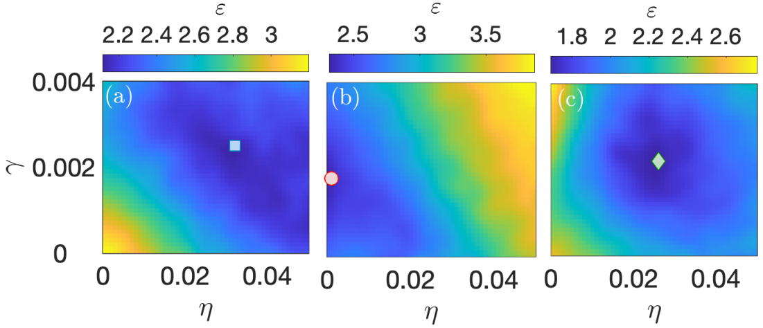
For the simulation results shown in Fig. 5 the magnitude of the mutual friction coefficient is identical for all three cases, . Curiously however, the on axis and off axis scenarios require different values of noise to capture the trends in the data. In experiment II, where the cluster is on axis, the decay is described purely by mutual friction, with , whereas in experiments I and V, where the cluster is off axis, significant diffusion is required, with . The noise is found to be crucial to reproducing the trends of the experimental data for the off-axis states; in particular, mutual friction alone yields essentially no decay of the dipole moment for reasonable values of , and also cannot reproduce the slight increase in the angular momentum per vortex observed in Fig. 5(c).
A more comprehensive fitting analysis, presented in Fig. 6, confirms this picture. Figure 6 shows estimated optimal values for and obtained by minimizing the sum-of-squares error between the theoretical and experimental values of , , and , i.e., by minimizing
| (14) |
where and . We use s, with the initial time chosen such that the experimental data could be used as the initial conditions, without needing to compensate for undercounting at early times. It is clear from Fig. 6 that the optimal value for is similar in all three cases. However, the on-axis case requires no noise while the off-axis cases require . The exact numerical values should be interpreted with some caution, as these fluctuate with the choice of initial conditions (roughly a factor of for different choices of ). Nonetheless, the on-axis case (experiment II) consistently yields , whereas the two off-axis cases (experiments I and V) yield .
The mutual friction term involving may be rigorously derived Törnkvist and Schröder 1997 from the damped Gross-Pitaevskii equation familiar from -field methods Blakie and Davis 2005; Gardiner et al. 2002; Gardiner and Davis 2003; Rooney et al. 2012, where describes the damping rate of the condensate due to Bose-enhanced collisions with a stationary thermal cloud Blakie et al. 2008. While we add the Brownian motion term as a phenomenological parameter, we note that thermally driven density and phase fluctuations of the condensate, which are neglected within a pure point-vortex treatment, will also contribute to the vortex dynamics Törnkvist and Schröder 1997; Groszek et al. 2018.
Our findings in this section show that Brownian motion is essential to capturing the thermal decay observed in global measures of the vortex distribution. This finding appears to be contrary to the standard paradigm of mutual friction (e.g., see Kim et al. 2016; Sachkou et al. 2019). While one might anticipate a fluctuation term based on the usual fluctuation-dissipation arguments, it should be noted that these arguments cannot be applied in a straightforward manner here; typically the competition between dissipation and noise serves to produce a steady thermal distribution, whereas here both terms are effectively dissipative — the equilibrium is one in which no vortices are present at all. In fact, by analogy with classical vortex methods for viscous fluids Chorin 2013, the noise can be interpreted as an effective viscosity. The noise is found to be necessary only for the off-axis states, which are at negative absolute temperature. A possible cause is that trap noise due to diffraction in the optical potentials may be more important at the trap edge. A more intriguing possibility is that the noise might be due to the negative-temperature vortex system being coupled to a positive-temperature phonon bath.
V Conclusions and outlook
We have experimentally studied equilibrium and nonequilibrium states of a chiral vortex gas confined within a disk-shaped atomic Bose-Einstein condensate. The steady-state distributions have been shown to be in quantitative agreement with the predictions of the microcanonical ensemble, at both positive and negative temperatures. While there is a small amount of dissipation present in the system, this is slow compared to the mixing timescale of the conservative vortex dynamics; this leads to the system slowly evolving through different microcanonical equilibria as time progresses. We have also quantified the sources of dissipation, showing that the dynamics of the quantum vortices are quantitatively described by point-vortex dynamics supplemented by thermal friction and Brownian motion.
We have found that the mean-field predictions for the vortex density describe our system remarkably well, despite the system containing only vortices, suggesting beyond-mean-field corrections may be negligible in much of the vortex gas phase diagram. While this might seem surprising in a low-dimensional system, we note that the long-range interactions mean that the vortices effectively have many nearest neighbors, supporting the use of a mean-field approach.
Note, however, the mean-field description cannot describe physics at the scales of the intervortex distance. This can become important, for example, at low energies, where the vortex distribution approaches the Rankine vortex [A, Table 1]. Recently, Bogatskiy and Weigmann Bogatskiy and Wiegmann 2019 have shown the Rankine vortex is expected to exhibit quantum Hall analog physics, including density oscillations on scales comparable to the intervortex distance, and quantized edge solitons. Our results in experiment II (also Ref Stockdale et al. 2020) show that the system is nearing the Rankine vortex regime, suggesting such physics is within reach experimentally.
Our results present atomic gas superfluids as complementary to existing platforms for the fundamental study of two-dimensional turbulence. The mean-field Poisson-Boltzmann equation, although originally developed for classical fluids, cannot be straightforwardly applied to the continuous vorticity distributions of classical fluids as it is derived from the point-vortex approximation Miller 1990; Robert 1991; Robert and Sommeria 1991. This is because the point-vortex approximation does not respect the conservation of other important quantities such as the peak vorticity and the so-called ‘Casimirs’ that are preserved by the full Euler equation Miller 1990; Robert and Sommeria 1991. By contrast, in our system the point-vortex approximation is an excellent description; for larger and lower dissipation, the Poisson-Boltzmann equation could in principle be applied with no fitted parameters. Another complementary aspect of our system is control over dimensionality; in two-dimensional classical fluid flows it is often difficult to determine the influence of the third dimension Tabeling and Cardoso 2012. While our particular system is quasi-2D, we note that quantum systems permit the complete freezing out of the third dimension to the zero-point motion Hadzibabic et al. 2006.
As Hamiltonian systems with long-range interactions are known to exhibit divergent thermalization times in the large-particle limit Levin et al. 2014; Pakter and Levin 2018, it would be interesting to experimentally probe systems with a larger number of vortices to test whether superfluids suffer the same issue. Here more complex routes to equilibrium (involving many cluster mergers) could be tested, to determine whether local entropy maxima such as vortex crystals Fine et al. 1995; Jin and Dubin 1998; Adriani et al. 2018, or nonequilibrium steady states such as core-halo states Pakter and Levin 2018 emerge in superfluid systems. The 2D quantum vortex gas presents a rather unique system to study turbulent phenomena; here, unlike in a classical, viscous fluid, the number of active degrees of freedom can be varied independently of the dissipation mechanism. In a viscous fluid both are controlled by the Reynolds number, . In 2D the number of active degrees of freedom scales as , while the energy dissipation rate scales as Batchelor 1969). In contrast, for the quantum vortex gas the dissipation rate from mutual friction is independent of the vortex number .
Future work on vortex matter may also provide new insights into the role of vortex mass in quantum fluids. Theoretical mass estimates range from to Simula 2018, while others argue the corrections do not affect the dynamics or are undefined Thouless and Anglin 2007; Lucas and Surówka 2014. Crucially, recall that the absence of vortex mass in Eq. (1) is the property that results in the bounded phase space Eq. (6) and hence the existence of negative-temperature states. For large enough mass, the mass-dependent cyclotron-like motion Driscoll and Fine 1990; Griffin et al. 2020; Richaud et al. 2020 would alter the equilibrium profiles and eventually destroy the negative-temperature states Smith and O’Neil 1990; our observations in agreement with massless vortices suggest that any vortex mass corrections are likely to be small.
The continued study of vortex matter will also benefit the growing interest in technological applications of atomtronic devices Eckel et al. 2016; Burchianti et al. 2018; Gauthier et al. 2019b, and renewed interest in nanomechanical resonators with superfluid helium Sachkou et al. 2019; Harris et al. 2016; Souris et al. 2017; He et al. 2020; Varga et al. 2020. These experiments suggest an enhanced understanding of superfluid turbulence will be required. Equilibrium theories of vortex matter may prove a useful tool in predicting the end states of turbulence in such applications provided fluid flows are sufficiently two dimensional — particularly in helium, where vortices cannot be directly imaged. As some systems are known to exhibit effective equilibria under steady driving and loss Foss-Feig et al. 2017, it would be interesting to consider the possibility of emergent equilibria in driven superfluid systems, such as the superfluid helium Helmholtz resonator recently studied in Ref. Varga et al. 2020.
Acknowledgements
We thank E. Kozik, N. Proukakis, and T. Simula for useful discussions. M.T.R. and T.W.N. thank the Institute for Nuclear Theory (INT) at the University of Washington for its kind hospitality and stimulating research environment at the INT-19-1a workshop, during which some of this research was undertaken. This research was supported in part by the INT’s U.S. Department of Energy Grant No. DE-FG02- 00ER41132. This research was supported by the Australian Research Council (ARC) Centre of Excellence for Engineered Quantum Systems (EQUS, CE170100009), and ARC Discovery Projects Grant DP160102085. This research was also partially supported by the ARC Centre of Excellence in Future Low-Energy Electronics Technologies (FLEET, project number CE170100039) and funded by the Australian Government. G.G. acknowledges the support of an Australian Government Research and Training Program Scholarship. XY acknowledges the support from NSAF with grant No. U1930403 and NSFC with grant No. 12175215. T.W.N. acknowledges the support of an ARC Future Fellowship FT190100306. Computing support was provided by the Getafix cluster at the University of Queensland.
VI Experimental procedure
Initial state preparation
A key ingredient for observing the predicted equilibrium vortex gas states, and the relaxation of nonequilibrium configurations, are experimental techniques that facilitate the injection of vortices with nearly arbitrary angular momentum and energy. The topological nature of single-quantized vortices means that they must be introduced from the boundary of the condensate. Since the DMD provides dynamic control of the potential, vortices can introduced into the condensate by “paddle” barriers that intersect the condensate edge and are stirred through the superfluid Gauthier et al. 2019a; Johnstone et al. 2019. The number of vortices in a cluster, and the cluster location, can be controlled by the speed and location of the paddle. A series of frames from GPE simulations of the vortex injection protocols are shown in Fig. 7, schematically illustrating the stirring schemes.
Experiment I: For injecting a single cluster, the experimental sequence follows: After transfer to the final potential, and a one-second equilibration period, the elliptically shaped paddle, with a major and minor axis of m and m, respectively, is swept through the Bose-Einstein condensate (BEC) at constant velocity; the paddle intersects the edge of the circular trap at its midpoint. The paddle sweep is defined by a set of 250 frames and the paddles sweep at a constant velocity (approximately , where ). After crossing the halfway point of their translation, the paddle is linearly ramped to zero intensity by reducing the major and minor axis widths to zero DMD pixels. The resulting vortex cluster is shown in the left column in Fig. 2.
Experiment II: For creating a vortex cluster on the axis of the disk trap, a different approach is used, as placement of the cluster immediately on axis via an external paddle is found to have poor repeatability. Following procedures for producing persistent currents in ring-trapped BECs Eckel et al. 2014; Wright et al. 2013, we first initialize the BEC in an annular trap, resulting from ramping on of an additional central barrier with m to the circular trap over 200 ms. Simultaneously, an elliptical stirring barrier that crosses the annulus is added, resulting in a split ring. The elliptical paddle has a major and minor axis of m and m respectively. Over a time of 400 ms, the stirring paddle is linearly accelerated at . While still moving the paddle at the final velocity, it is then ramped off by reducing both the barrier width and length over 100 ms. After a 400-ms period of equilibration in the annular trap, the central barrier is then removed over 200 ms by linearly reducing its radius to zero. This results in a high-energy cluster of approximately 12 vortices localized to the trap center. During the retraction of the paddle, sometimes one or two extraneous vortices of the same sign are produced, however, this is later shown to have little effect on the dynamics of the central cluster. Energy damping results in the cluster gradually spreading, and after s the vortices can be easily resolved.
Experiment III, IV: To realize the Gaussian and near-Riccati equilibrium states, a third stirring technique was used, based on the methods of Ref. Wilson et al. 2021. Two pinning beams are spiraled into the condensate until separated by a distance , resulting in two multicharge vortices. On removing the pins, the multicharge vortices break up into two distinct clusters of approximately 7 vortices each, before merging into a single cluster over the course of the dynamics. The stirring process occurs as follows. The beams are initially located on the edge of the condensate and rotate at a constant frequency, while the radial position of the beams is linearly ramped from to over ms, resulting in spiral paths. For experiment III, the stirring beams have a diameter of m, rotated at Hz, and the final spacing is m. On reaching their final locations, the radii of the pinning potentials are linearly ramped to zero over ms. For experiment IV, the stirring beams have a diameter of 30 m, rotated at Hz, and the final spacing is m.
Experiment V: This scenario uses the same technique as experiment I; by using two paddles with the same parameters, but propagating in opposite directions, two same-sign vortex clusters can be realized.
Experimental data collection and vortex imaging
The sensitivity of the vortex configurations to density gradients requires fine control of the magnetic levitation field to ensure a uniform BEC density. This was achieved by applying small magnetic correction gradients and ensuring that the central vortex cluster created in experiment II remains centered in the BEC over the initial 500 ms of evolution. By periodically repeating this calibration procedure, we find that the experiment exhibits slow, small-scale drifts in the density balance, which settle after an initial period of approximately 8 h of running. The data presented in the main text are thus collected in a continuous period subsequent to this warm-up.
High-resolution images of the BEC and vortex cores are obtained after a short, 3-ms time of flight that allows the vortex cores to expand and become visible. The radial distribution of the condensate is essentially unchanged from this expansion. Dark-ground Faraday imaging Bradley et al. 1997 is used, with light detuned by 220 MHz from the 87Rb transition, in the 80-G magnetic field resulting from the magnetic compensation of gravity. The vortex positions are then obtained using a Gaussian fitting algorithm (Rakonjac et al. 2016; Gauthier et al. 2019a). The Faraday imaging light is sufficiently closely detuned that the images of the BEC are destructive.
For experiments I, II, and V, up to 40 images are collected for each hold time in 250-ms increments up to the maximum time of 6.75 s. This amount of data generates reliable statistics for vortex distributions as a function of time. The resulting histograms for the several hold times for experiment I are shown in Fig. 2.
The results of Sec. IV confirm that our system is well described by a simple point-vortex model, and that the dissipative losses are sufficiently weak at late times that the system can be treated as being in approximate microcanonical equilibrium for the time period 3.25 s – 6.75 s. The histograms shown in Fig. 3 for experiments II and V thus show the average quasiequilibrium vortex density histograms for the images collected for s.
In contrast, we do not record time series data for experiments III and IV. Instead, sets of images are collected for the initial state and at a single, sufficiently long hold time such that quasiequilibrium has been reached. For experiment III, 120 images are collected at a 4-s hold time, and for experiment IV, 361 images were collected at a 1.5-s hold time.

GPE modeling of stirring protocols
We simulated the initial vortex injection using a phenomenologically damped GPE (dGPE) model. Working in length units of the healing length and time units defined by the chemical potential , we simulate the following equation for
| (15) |
where is the external potential and is a phenomenological damping factor of which matches the thermal friction coefficient observed in the experiment. Note that the Brownian motion term is not included in this model, as these effects are not significant to the stirring dynamics. The circular trapping and pinning potentials and the elliptical stirring potentials are modeled as hard-wall potentials of the general form
| (16) |
where is the strength of the potential, and are the semimajor and semiminor axis respectively, and to allow for translation or and to allow for rotations by angle , and controls the steepness of the potential. Figure 7 shows the resulting condensate density snapshots from simulating the stirring protocols with similar parameters to those performed in the experiment. All vortices injected were of the same sign. Movies of dGPE simulations of the vortex injection methods are provided in the Supplemental Material SM.
VII Solution of Poisson-Boltzmann equation
To solve the Poisson equation given by
| (17) |
subject to the boundary conditions and the constraints of prescribed angular momentum (angular impulse), energy, and normalisation given by
| (18) |
we adapt the method described in Ref. Turkington and Whitaker 1996. First, we represent the stream function in space using a Fourier series decomposition in terms of the azimuthal angle so that
| (19) |
The above equation then reduces to
| (20) |
To satisfy the boundary condition, we require that , and . For , we set where a prime denotes differentiation with respect to the radius . This radial equation is then discretized using a centered finite-differencing scheme. The resulting discretized equation can be inverted to recover the streamfunction from the vortex density field.
To find a self-consistent solution of the Poisson-Boltzmann equation subject to the constraints given, we define the functional
| (21) |
where . We want to find such that is stationary so that . This requires that
| (22) |
which implies that
| (23) |
It follows that we can rewrite the three constraints in the form
| (24) |
We note that the constraints and are both linear in the vortex density . However, the constraint for the energy is nonlinear since it can expressed in terms of the Green’s function of the Laplacian operator as
| (25) |
where is the 2D Green’s function for a point vortex confined within a circular disk Newton 2013. Linearizing the energy about the state , we obtain
| (26) |
The linearized constraint on energy is then given by
| (27) |
We can now rewrite the three constraints in the linearized form
| (28) |
where and . The advantage of casting the constraints in this form is that we can now proceed to update the system of Lagrange multipliers by using a Newton-Raphson iteration scheme. Alternatively, given that the constraints are now expressed in terms of a gradient operator, a gradient descent algorithm can now be used to give
| (29) |
where is a relaxation parameter . In practice, we use a gradient descent algorithm to obtain a good estimate of followed by a Newton-Raphson scheme in order to accelerate convergence. The Newton-Raphson scheme requires the evaluation of the Hessian of that we denote by . The updates can then be evaluated as
| (30) |
The iterations are stopped once the values for , , and converge to within a tolerance of .
To obtain the branch corresponding to axisymmetric (centered) flows, we solve the above by setting the coefficients of all modes corresponding to to zero. To find the symmetric and off-centered maximum entropy solutions, we typically started with an exact solution such as the Gaussian profile corresponding to and then trace out the branches by varying the energy for fixed and .
References
- Thalabard et al. (2015) Simon Thalabard, Brice Saint-Michel, Eric Herbert, François Daviaud, and Bérengère Dubrulle, “A statistical mechanics framework for the large-scale structure of turbulent von Kármán flows,” New Journal of Physics 17, 063006 (2015).
- Frisch (1995) Uriel Frisch, Turbulence: the legacy of AN Kolmogorov (Cambridge university press, 1995).
- Batchelor (1953) George Keith Batchelor, The theory of homogeneous turbulence (Cambridge university press, 1953).
- Kraichnan (1967) Robert H Kraichnan, “Inertial ranges in two-dimensional turbulence,” The Physics of Fluids 10, 1417–1423 (1967).
- Batchelor (1969) G. K. Batchelor, “Computation of the energy spectrum in homogeneous two‐dimensional turbulence,” The Physics of Fluids 12, II–233–II–239 (1969).
- Sarid et al. (2004a) Eli Sarid, Catalin Teodorescu, Philip S. Marcus, and Joel Fajans, “Breaking of Rotational Symmetry in Cylindrically Bounded 2D Electron Plasmas and 2D Fluids,” Physical Review Letters 93, 215002 (2004a).
- Rodgers et al. (2009) D. J. Rodgers, S. Servidio, W. H. Matthaeus, D. C. Montgomery, T. B. Mitchell, and T. Aziz, “Hydrodynamic relaxation of an electron plasma to a near-maximum entropy state,” Physical Review Letters 102, 244501 (2009).
- Kellay (2017) H. Kellay, “Hydrodynamics experiments with soap films and soap bubbles: A short review of recent experiments,” Physics of Fluids 29, 111113 (2017).
- Hansen et al. (1998) A. E. Hansen, D. Marteau, and P. Tabeling, “Two-dimensional turbulence and dispersion in a freely decaying system,” Phys. Rev. E 58, 7261–7271 (1998).
- Adriani et al. (2018) Alberto Adriani, A Mura, G Orton, C Hansen, F Altieri, M. L. Moriconi, J Rogers, G Eichstädt, T Momary, Andrew P Ingersoll, et al., “Clusters of cyclones encircling Jupiter’s poles,” Nature 555, 216 (2018).
- Bouchet and Sommeria (2002) F. Bouchet and J. Sommeria, “Emergence of intense jets and Jupiter’s Great Red Spot as maximum-entropy structures,” Journal of Fluid Mechanics 464, 165–207 (2002).
- Onsager (1949) Lars Onsager, “Statistical hydrodynamics,” Il Nuovo Cimento (1943-1954) 6, 279–287 (1949).
- Joyce and Montgomery (1973) Glenn Joyce and David Montgomery, “Negative temperature states for the two-dimensional guiding-centre plasma,” Journal of Plasma Physics 10, 107–121 (1973).
- Edwards and Taylor (1974) S. F. Edwards and J. B. Taylor, “Negative temperature states of two-dimensional plasmas and vortex fluids,” Proceedings of the Royal Society of London. Series A, Mathematical and Physical Sciences 336, 257–271 (1974).
- Kraichnan (1975) R. H. Kraichnan, “Statistical dynamics of two-dimensional flow,” J. Fluid Mech. 67, 155–175 (1975).
- Miller (1990) Jonathan Miller, “Statistical mechanics of Euler equations in two dimensions,” Physical Review Letters 65, 2137–2140 (1990).
- Robert (1991) Raoul Robert, “A maximum-entropy principle for two-dimensional perfect fluid dynamics,” Journal of Statistical Physics 65, 531–553 (1991).
- Robert and Sommeria (1991) R. Robert and J. Sommeria, “Statistical equilibrium states for two-dimensional flows,” Journal of Fluid Mechanics 229, 291–310 (1991).
- Maestrini and Salman (2019) Davide Maestrini and Hayder Salman, “Entropy of negative temperature states for a point vortex gas,” Journal of Statistical Physics 176, 981–1008 (2019).
- Denoix (1992) Marie-Alice Denoix, Experimental study of stable structures in two-dimensional turbulence - Comparison with a statistical mechanical theory, Thesis, Institut National Polytechnique de Grenoble (1992).
- Matthaeus et al. (1991) W.H. Matthaeus, W.T. Stribling, D. Martinez, S. Oughton, and D. Montgomery, “Decaying, two-dimensional, Navier-Stokes turbulence at very long times,” Physica D: Nonlinear Phenomena 51, 531 – 538 (1991).
- Tabeling (2002) Patrick Tabeling, “Two-dimensional turbulence: a physicist approach,” Physics Reports 362, 1–62 (2002).
- Sarid et al. (2004b) Eli Sarid, Catalin Teodorescu, Philip S. Marcus, and Joel Fajans, “Breaking of rotational symmetry in cylindrically bounded 2D electron plasmas and 2D fluids,” Physical Review Letters 93, 215002 (2004b).
- Driscoll and Fine (1990) C. F. Driscoll and K. S. Fine, “Experiments on vortex dynamics in pure electron plasmas,” Physics of Fluids B: Plasma Physics 2, 1359–1366 (1990).
- Carnevale et al. (1992) G. F. Carnevale, J. C. McWilliams, Y. Pomeau, J. B. Weiss, and W. R. Young, “Rates, pathways, and end states of nonlinear evolution in decaying two-dimensional turbulence: Scaling theory versus selective decay,” Physics of Fluids A: Fluid Dynamics 4, 1314–1316 (1992).
- Marteau et al. (1995) D. Marteau, O. Cardoso, and P. Tabeling, “Equilibrium states of two-dimensional turbulence: An experimental study,” Physical Review E 51, 5124–5127 (1995).
- Huang and Driscoll (1994) X.-P. Huang and C. F. Driscoll, “Relaxation of 2D turbulence to a metaequilibrium near the minimum enstrophy state,” Physical Review Letters 72, 2187–2190 (1994).
- Pakter and Levin (2018) Renato Pakter and Yan Levin, “Nonequilibrium statistical mechanics of two-dimensional vortices,” Physical Review Letters 121, 020602 (2018).
- Levin et al. (2014) Yan Levin, Renato Pakter, Felipe B Rizzato, Tarcísio N Teles, and Fernanda PC Benetti, “Nonequilibrium statistical mechanics of systems with long-range interactions,” Physics Reports 535, 1–60 (2014).
- Brands et al. (1999) H. Brands, S. R. Maassen, and H. J. H. Clercx, “Statistical-mechanical predictions and Navier-Stokes dynamics of two-dimensional flows on a bounded domain,” Phys. Rev. E 60, 2864–2874 (1999).
- Li and Montgomery (1996) Shuojun Li and David Montgomery, “Decaying two-dimensional turbulence with rigid walls,” Physics Letters A 218, 281–291 (1996).
- Van Heijst et al. (2006) G. J. F. Van Heijst, H. J. H. Clercx, and D. Molenaar, “The effects of solid boundaries on confined two-dimensional turbulence,” Journal of Fluid Mechanics 554, 411–431 (2006).
- Gaunt et al. (2013) Alexander L. Gaunt, Tobias F. Schmidutz, Igor Gotlibovych, Robert P. Smith, and Zoran Hadzibabic, “Bose-Einstein Condensation of Atoms in a Uniform Potential,” Phys. Rev. Lett. 110, 200406 (2013).
- Chomaz et al. (2015) Lauriane Chomaz, Laura Corman, Tom Bienaimé, Rémi Desbuquois, Christof Weitenberg, Sylvain Nascimbene, Jérôme Beugnon, and Jean Dalibard, “Emergence of coherence via transverse condensation in a uniform quasi-two-dimensional Bose gas,” Nature Communications 6, 1–10 (2015).
- Gauthier et al. (2016) G. Gauthier, I. Lenton, N. McKay Parry, M. Baker, M. J. Davis, H. Rubinsztein-Dunlop, and T. W. Neely, “Direct imaging of a digital-micromirror device for configurable microscopic optical potentials,” Optica 3, 1136–1143 (2016).
- Mukherjee et al. (2017) Biswaroop Mukherjee, Zhenjie Yan, Parth B Patel, Zoran Hadzibabic, Tarik Yefsah, Julian Struck, and Martin W Zwierlein, “Homogeneous atomic Fermi gases,” Physical Review Letters 118, 123401 (2017).
- Tajik et al. (2019) Mohammadamin Tajik, Bernhard Rauer, Thomas Schweigler, Federica Cataldini, João Sabino, Frederik S Møller, Si-Cong Ji, Igor E Mazets, and Jörg Schmiedmayer, “Designing arbitrary one-dimensional potentials on an atom chip,” Optics Express 27, 33474–33487 (2019).
- Navon et al. (2021) Nir Navon, Robert P. Smith, and Zoran Hadzibabic, “Quantum gases in optical boxes,” Nature Physics 17, 1334–1341 (2021).
- Navon et al. (2016) Nir Navon, Alexander L. Gaunt, Robert P. Smith, and Zoran Hadzibabic, “Emergence of a Turbulent Cascade in a Quantum Gas,” Nature 539, 72–75 (2016).
- Navon et al. (2019) Nir Navon, Christoph Eigen, Jinyi Zhang, Raphael Lopes, Alexander L. Gaunt, Kazuya Fujimoto, Makoto Tsubota, Robert P. Smith, and Zoran Hadzibabic, “Synthetic dissipation and cascade fluxes in a turbulent quantum gas,” Science 366, 382–385 (2019).
- Glidden et al. (2021) Jake AP Glidden, Christoph Eigen, Lena H Dogra, Timon A Hilker, Robert P Smith, and Zoran Hadzibabic, “Bidirectional dynamic scaling in an isolated bose gas far from equilibrium,” Nature Physics 17, 457–461 (2021).
- Gauthier et al. (2019a) Guillaume Gauthier, Matthew T Reeves, Xiaoquan Yu, Ashton S Bradley, Mark A Baker, Thomas A Bell, Halina Rubinsztein-Dunlop, Matthew J Davis, and Tyler W Neely, “Giant vortex clusters in a two-dimensional quantum fluid,” Science 364, 1264–1267 (2019a).
- Johnstone et al. (2019) Shaun P Johnstone, Andrew J Groszek, Philip T Starkey, Christopher J Billington, Tapio P Simula, and Kristian Helmerson, “Evolution of large-scale flow from turbulence in a two-dimensional superfluid,” Science 364, 1267–1271 (2019).
- Stockdale et al. (2020) Oliver R. Stockdale, Matthew T. Reeves, Xiaoquan Yu, Guillaume Gauthier, Kwan Goddard-Lee, Warwick P. Bowen, Tyler W. Neely, and Matthew J. Davis, “Universal dynamics in the expansion of vortex clusters in a dissipative two-dimensional superfluid,” Physical Review Research 2, 033138 (2020).
- Kwon et al. (2021) W. J. Kwon, G. Del Pace, K. Xhani, L. Galantucci, A. Muzi Falconi, M. Inguscio, F. Scazza, and G. Roati, “Sound emission and annihilations in a programmable quantum vortex collider,” Nature 600, 64–69 (2021).
- Fetter (1966) Alexander L. Fetter, “Vortices in an Imperfect Bose Gas. IV. Translational Velocity,” Physical Review 151, 100–104 (1966).
- Groszek et al. (2018) Andrew J Groszek, David M Paganin, Kristian Helmerson, and Tapio P Simula, “Motion of vortices in inhomogeneous Bose-Einstein condensates,” Physical Review A 97, 023617 (2018).
- Dritschel et al. (2015) David G. Dritschel, Marcello Lucia, and Andrew C. Poje, “Ergodicity and spectral cascades in point vortex flows on the sphere,” Phys. Rev. E 91, 063014 (2015).
- Esler and Ashbee (2015) J. G. Esler and T. L. Ashbee, “Universal statistics of point vortex turbulence,” J. Fluid Mech. 779, 275–308 (2015).
- Salman and Maestrini (2016) Hayder Salman and Davide Maestrini, “Long-range ordering of topological excitations in a two-dimensional superfluid far from equilibrium,” Physical Review A 94, 043642 (2016).
- Yu et al. (2016) Xiaoquan Yu, Thomas P. Billam, Jun Nian, Matthew T. Reeves, and Ashton S. Bradley, “Theory of the vortex-clustering transition in a confined two-dimensional quantum fluid,” Physical Review A 94, 023602 (2016).
- Smith (1989) R A Smith, “Phase-Transition Behavior in a Negative-Temperature Guiding-Center Plasma,” Physical Review Letters 63, 1479–1482 (1989).
- Newton (2013) Paul K. Newton, The N-Vortex Problem: Analytical Techniques, Vol. 145 (Springer Science & Business Media, 2013).
- Smith and O’Neil (1990) Ralph A. Smith and Thomas M. O’Neil, “Nonaxisymmetric thermal equilibria of a cylindrically bounded guiding-center plasma or discrete vortex system,” Physics of Fluids B: Plasma Physics 2, 2961–2975 (1990).
- (55) is often referred to as the angular momentum Newton 2013; Aref 1979. The distinction is not so important when applying the point-vortex model to the dynamics of a classical Euler fluid (where the vortex number is conserved), but is for a superfluid as vortex annihilation can occur at the boundary; here varies continuously as a vortex leaves at the boundary, whereas changes discontinuously.
- (56) Note however that for a given solution does not necessarily correspond to any particular physical rotation rate in the system; see Ref. Smith and O’Neil 1990.
- (57) This behaviour follows from the fact that below the off-axis transition the vortex positions are approximately normally distributed about the origin, with the width of the normal distribution determined by the angular momentum.
- Samson (2012) Edward Carlo Copon Samson, Generating and manipulating quantized vortices in highly oblate Bose-Einstein condensates, Ph.D. thesis, The University of Arizona (2012).
- Bradley et al. (1997) Curtis Charles Bradley, C. A. Sackett, and R. G. Hulet, “Bose-Einstein condensation of lithium: Observation of limited condensate number,” Physical Review Letters 78, 985 (1997).
- Rakonjac et al. (2016) A. Rakonjac, A. L. Marchant, T. P. Billam, J. L. Helm, M. M. H. Yu, S. A. Gardiner, and S. L. Cornish, “Measuring the disorder of vortex lattices in a Bose-Einstein condensate,” Physical Review A 93, 013607 (2016).
- Chavanis and Sommeria (1996) Pierre-Henri Chavanis and Joel Sommeria, “Classification of self-organized vortices in two-dimensional turbulence: the case of a bounded domain,” Journal of Fluid Mechanics 314, 267–297 (1996).
- Weiss and McWilliams (1993) Jeffrey B. Weiss and James C. McWilliams, “Temporal scaling behavior of decaying two‐dimensional turbulence,” Physics of Fluids A: Fluid Dynamics 5, 608–621 (1993).
- Simula et al. (2014) Tapio Simula, Matthew J. Davis, and Kristian Helmerson, “Emergence of order from turbulence in an isolated planar superfluid,” Physical Review Letters 113, 165302 (2014).
- Billam et al. (2015) T. P. Billam, M. T. Reeves, and A. S. Bradley, “Spectral energy transport in two-dimensional quantum vortex dynamics,” Phys. Rev. A 91, 023615 (2015).
- (65) The positions of the additional vortices were determined by using the experimental histograms [cf. Fig. 2] as probability distributions for rejection sampling. For experiments I and V, one additional vortex was added to each experimental run. For experiment II, between 2 and 3 vortices were added with equal probability.
- Törnkvist and Schröder (1997) Ola Törnkvist and Elsebeth Schröder, “Vortex dynamics in dissipative systems,” Physical Review Letters 78, 1908 (1997).
- Blakie and Davis (2005) P Blair Blakie and Matthew J Davis, “Projected Gross-Pitaevskii equation for harmonically confined Bose gases at finite temperature,” Physical Review A 72, 063608 (2005).
- Gardiner et al. (2002) C W Gardiner, J R Anglin, and T I A Fudge, “The Stochastic Gross-Pitaevskii equation,” Journal of Physics B: Atomic, Molecular and Optical Physics 35, 1555–1582 (2002).
- Gardiner and Davis (2003) C. W. Gardiner and M. J. Davis, “The stochastic Gross–Pitaevskii equation: Ii,” Journal of Physics B: Atomic, Molecular and Optical Physics 36, 4731 (2003).
- Rooney et al. (2012) S. J. Rooney, P. B. Blakie, and A. S. Bradley, “Stochastic projected Gross-Pitaevskii equation,” Physical Review A 86, 053634 (2012).
- Blakie et al. (2008) P. B. Blakie, A. S. Bradley, M. J. Davis, R. J. Ballagh, and C. W. Gardiner, “Dynamics and statistical mechanics of ultra-cold bose gases using c-field techniques,” Advances in Physics 57, 363–455 (2008).
- Kim et al. (2016) Joon Hyun Kim, Woo Jin Kwon, and Y. Shin, “Role of thermal friction in relaxation of turbulent Bose-Einstein condensates,” Physical Review A 94, 033612 (2016).
- Sachkou et al. (2019) Yauhen P. Sachkou, Christopher G. Baker, Glen I. Harris, Oliver R. Stockdale, Stefan Forstner, Matthew T. Reeves, Xin He, David L. McAuslan, Ashton S. Bradley, Matthew J. Davis, and Warwick P. Bowen, “Coherent vortex dynamics in a strongly interacting superfluid on a silicon chip,” Science 366, 1480–1485 (2019).
- Chorin (2013) Alexandre J Chorin, Vorticity and turbulence, Vol. 103 (Springer Science & Business Media, 2013).
- Bogatskiy and Wiegmann (2019) A. Bogatskiy and P. Wiegmann, “Edge wave and boundary layer of vortex matter,” Physical Review Letters 122, 214505 (2019).
- Tabeling and Cardoso (2012) Patrick Tabeling and O Cardoso, Turbulence: a tentative dictionary, Vol. 341 (Springer Science & Business Media, 2012).
- Hadzibabic et al. (2006) Zoran Hadzibabic, Peter Krüger, Marc Cheneau, Baptiste Battelier, and Jean Dalibard, “Berezinskii–Kosterlitz–Thouless crossover in a trapped atomic gas,” Nature 441, 1118–1121 (2006).
- Fine et al. (1995) K. S. Fine, A. C. Cass, W. G. Flynn, and C. F. Driscoll, “Relaxation of 2D Turbulence to Vortex Crystals,” Physical Review Letters 75, 3277–3280 (1995).
- Jin and Dubin (1998) D. Z. Jin and Daniel H. E. Dubin, “Regional maximum entropy theory of vortex crystal formation,” Physical Review Letters 80, 4434–4437 (1998).
- Simula (2018) Tapio Simula, “Vortex mass in a superfluid,” Physical Review A 97, 023609 (2018).
- Thouless and Anglin (2007) D. J. Thouless and J. R. Anglin, “Vortex mass in a superfluid at low frequencies,” Physical Review Letters 99, 105301 (2007).
- Lucas and Surówka (2014) Andrew Lucas and Piotr Surówka, “Sound-induced vortex interactions in a zero-temperature two-dimensional superfluid,” Physical Review A 90, 053617 (2014).
- Griffin et al. (2020) Adam Griffin, Vishwanath Shukla, Marc-Etienne Brachet, and Sergey Nazarenko, “Magnus-force model for active particles trapped on superfluid vortices,” Physical Review A 101, 053601 (2020).
- Richaud et al. (2020) Andrea Richaud, Vittorio Penna, Ricardo Mayol, and Montserrat Guilleumas, “Vortices with massive cores in a binary mixture of Bose-Einstein condensates,” Physical Review A 101, 013630 (2020).
- Eckel et al. (2016) S Eckel, Jeffrey G Lee, F Jendrzejewski, C. J. Lobb, G. K. Campbell, and W. T. Hill III, “Contact resistance and phase slips in mesoscopic superfluid-atom transport,” Physical Review A 93, 063619 (2016).
- Burchianti et al. (2018) A Burchianti, F Scazza, A Amico, G Valtolina, J. A. Seman, C Fort, M Zaccanti, M Inguscio, and G Roati, “Connecting dissipation and phase slips in a Josephson junction between fermionic superfluids,” Physical Review Letters 120, 025302 (2018).
- Gauthier et al. (2019b) Guillaume Gauthier, Stuart S Szigeti, Matthew T Reeves, Mark Baker, Thomas A Bell, Halina Rubinsztein-Dunlop, Matthew J Davis, and Tyler W Neely, “Quantitative Acoustic Models for Superfluid Circuits,” Physical Review Letters 123, 260402 (2019b).
- Harris et al. (2016) GI Harris, DL McAuslan, E Sheridan, Y Sachkou, C Baker, and WP Bowen, “Laser cooling and control of excitations in superfluid helium,” Nature Physics 12, 788–793 (2016).
- Souris et al. (2017) F. Souris, X. Rojas, P. H. Kim, and J. P. Davis, “Ultralow-dissipation superfluid micromechanical resonator,” Physical Review Applied 7, 044008 (2017).
- He et al. (2020) Xin He, Glen I Harris, Christopher G Baker, Andreas Sawadsky, Yasmine L Sfendla, Yauhen P Sachkou, Stefan Forstner, and Warwick P Bowen, “Strong optical coupling through superfluid brillouin lasing,” Nature Physics 16, 417–421 (2020).
- Varga et al. (2020) E. Varga, V. Vadakkumbatt, A. J. Shook, P. H. Kim, and J. P. Davis, “Observation of bistable turbulence in quasi-two-dimensional superflow,” Phys. Rev. Lett. 125, 025301 (2020).
- Foss-Feig et al. (2017) M. Foss-Feig, P. Niroula, J. T. Young, M. Hafezi, A. V. Gorshkov, R. M. Wilson, and M. F. Maghrebi, “Emergent equilibrium in many-body optical bistability,” Physical Review A 95, 043826 (2017).
- Eckel et al. (2014) Stephen Eckel, Jeffrey G Lee, Fred Jendrzejewski, Noel Murray, Charles W Clark, Christopher J Lobb, William D Phillips, Mark Edwards, and Gretchen K Campbell, “Hysteresis in a quantized superfluid ‘atomtronic’ circuit,” Nature 506, 200 (2014).
- Wright et al. (2013) Kevin C Wright, RB Blakestad, C. J. Lobb, W. D. Phillips, and G. K. Campbell, “Driving phase slips in a superfluid atom circuit with a rotating weak link,” Physical Review Letters 110, 025302 (2013).
- Wilson et al. (2021) Kali E Wilson, E Samson, Zachary L Newman, and Brian P Anderson, “Generation of high winding-number superfluid circulation in Bose-Einstein condensates,” arXiv preprint arXiv:2109.12945 (2021).
- (96) See Supplemental Material at [URL will be inserted by publisher] for movies of damped GPE simulations of the three stirring protocols.
- Turkington and Whitaker (1996) Bruce Turkington and Nathaniel Whitaker, “Statistical equilibrium computations of coherent structures in turbulent shear layers,” SIAM Journal on Scientific Computing 17, 1414–1433 (1996).
- Aref (1979) Hassan Aref, “Motion of three vortices,” The Physics of Fluids 22, 393–400 (1979).