A meta-inference framework to integrate multiple external models into a current study

Let $\rm Y$ denote the outcome of interest, which can be either continuous or binary. $\rm\mathbf{X}$ is a set of p standard variables and let $\rm B$ denote a new biomarker. Our target of interest is the mean structure of $\rm Y|\mathbf{X},B$:

where $g$ is the known link function. We assume that a small dataset of size n with variables $\rm Y,\mathbf{X}$ and a new covariate $\rm B$ is available to us for building model 2.1. For each external study k, k $\in\rm\{2,...,K\}$, a prediction model for the same outcome $\rm Y$ has been built using predictors $\rm\mathbf{X}_{k}$, a subset of the internal $\mathbf{X}$. Each external model may use slightly different predictors to predict $\rm Y$:

where $\rm p_{k}\subseteq p$ is the dimension of $\rm\mathbf{X}_{k}$. We assume that the distribution of $\rm Y|\mathbf{X},B$ is correctly specified, but the external $\rm Y|\mathbf{X}_{k}$ distributions need not be.

We assume K large, well-characterized previous studies from the external populations describe the provided information on the calculated distribution of $\rm Y|\mathbf{X}_{k}$. These information will come in the forms of estimated model parameters $\rm\hat{\boldsymbol{\beta}}_{k}$. The goal is to develop a framework, in which we can utilize all K external $\rm\hat{\boldsymbol{\beta}}_{k}$’s to improve the estimation efficiency of the internal study.

We introduce some of the important notation that will frequently appear in later sections:

• •

  $\rm f_{\beta}(Y|X_{k})$: the study-specific distribution of the $\rm k^{th}$ external model $\rm Y|\mathbf{X}_{k}$;

• •

  $\rm f_{\gamma}(Y|X,B)$: distribution of the target model $\rm Y|\mathbf{X},B$;

• •

  $\rm\hat{\boldsymbol{\gamma}}_{I}$: the unconstrained estimator by using the internal data only;

• •

  $\rm\hat{\boldsymbol{\gamma}}_{CML}$: the constrained semi-parametric maximum likelihood estimator (CSPML) proposed by Chatterjee and others 2016;

• •

  $\rm\hat{\boldsymbol{\gamma}}_{EB}$: the empirical Bayes (EB) estimator proposed by Estes and others 2017.

The proposed method was developed on the foundation of two existing methods, the CSPML approach (Chatterjee and others 2016) and the EB approach (Estes and others 2017). The CSPML estimator considered the same problem described here in a special case where K=1; and EB estimator applied the empirical Bayes method to CSPML, calibrating the potential bias due to non-transportability. Therefore, it is necessary to introduce these two core methods first before considering the $\rm K>1$ situation.

In the CSPML, the proposed estimator $\rm\hat{\boldsymbol{\gamma}}_{CML}$ incorporates the external regression coefficients to calibrate the current regression model. Denote $\rm U_{\beta}(Y|X)$ as the score function of the external $\rm Y|X;\beta$ model. It converts the external model parameter $\rm\hat{\boldsymbol{\beta}}$ to a constraint by connecting the external score function with the target distribution $\rm f_{\gamma}(Y|X,B)$:

where $\rm dF(X,B)$ is the empirical probability distribution $\rm p_{i}=Pr(X=X_{i},B=B_{i})$ for the internal observations and $\rm\sum_{i=1}^{n}p_{i}=1$. Then $\rm\hat{\boldsymbol{\gamma}}_{CML}$ was obtained using Lagrange multipliers by solving the following Lagrangian function:

Chatterjee and others 2016 provided the asymptotic variance of $\rm\hat{\boldsymbol{\gamma}}_{CML}$, showing the efficiency gain of $\rm\hat{\boldsymbol{\gamma}}_{CML}$ compared to $\rm\hat{\boldsymbol{\gamma}}_{I}$.

Estes and others 2017 showed that in the CSPML approach, the strict assumption of the identical joint distribution of (Y,X,B) between the internal and the external population (also known as the full transportable assumption of the joint distribution of [Y,X,B]) is hard to satisfy in reality, and ignoring it can lead to substantial bias. Assuming the target conditional distribution ($\rm Y|X,B;\gamma$) is correctly specified in the internal study and the underlying true parameter $\rm\gamma$ follows a stochastic framework, Estes and others 2017 proposed an empirical Bayes (EB) estimator $\rm\hat{\boldsymbol{\gamma}}_{EB}$, which can be viewed as a matrix-weighted average of the internal estimate $\rm\hat{\boldsymbol{\gamma}}_{I}$ and the CSPML estimator $\rm\hat{\boldsymbol{\gamma}}_{CML}$. The EB estimator uses the difference $\rm\hat{\boldsymbol{\gamma}}_{I}-\hat{\boldsymbol{\gamma}}_{CML}$ to measure the distributional similarity of the joint distribution (Y, X, B) between the internal and the external population, and will down-weight $\rm\hat{\boldsymbol{\gamma}}_{CML}$ if the lack of full transportability leads to a poor estimate. Therefore, the EB estimator is robust to departures from full transportability assumption in specific external populations. The features and assumptions for the CSPML, the EB and the proposed estimators are summarized in Table A1 in Appendix A of the Supplementary Material.

Specifically, the EB approach first posits a stochastic framework connecting the internal estimator $\rm\hat{\boldsymbol{\gamma}}_{I}$ and the underlying true parameter $\rm\boldsymbol{\gamma}\sim N(\boldsymbol{\gamma}_{0},\mathbf{A})$ for some covariance matrix $\rm\mathbf{A}$. Since $\begin{cases}\rm\boldsymbol{\gamma}\sim N(\boldsymbol{\gamma}_{0},\mathbf{A})\\ \rm\hat{\boldsymbol{\gamma}}_{I}|\boldsymbol{\gamma}~N(\boldsymbol{\gamma},\mathbf{\Sigma})\end{cases}$, the posterior Bayes estimate of $\rm\boldsymbol{\gamma}$ equals to $\rm\mathbf{A}(\boldsymbol{\Sigma}+\mathbf{A})^{-1}\hat{\boldsymbol{\gamma}}_{I}+\boldsymbol{\Sigma}(\boldsymbol{\Sigma}+\mathbf{A})^{-1}\boldsymbol{\gamma}_{0}$. Replacing $\rm\boldsymbol{\gamma}_{0}$ with the CSPML estimator $\rm\hat{\boldsymbol{\gamma}}_{CML}$ and empirically estimating $\rm\mathbf{A}$ and $\rm\boldsymbol{\Sigma}$, we obtain the EB estimator $\rm\hat{\boldsymbol{\gamma}}_{EB}=\hat{\mathbf{A}}(\hat{\boldsymbol{\Sigma}}+\hat{\mathbf{A}})^{-1}\hat{\boldsymbol{\gamma}}_{I}+\hat{\boldsymbol{\Sigma}}(\hat{\boldsymbol{\Sigma}}+\hat{\mathbf{A}})^{-1}\hat{\boldsymbol{\gamma}}_{CML}\overset{\text{def}}{=}\rm\hat{\mathbf{W}}\boldsymbol{\hat{\gamma}}_{I}+(I-\hat{\mathbf{W}})\boldsymbol{\hat{\gamma}}_{CML}$, where $\rm\hat{\mathbf{A}}=(\boldsymbol{\hat{\gamma}}_{I}-\boldsymbol{\hat{\gamma}}_{CML})(\boldsymbol{\hat{\gamma}}_{I}-\boldsymbol{\hat{\gamma}}_{CML})^{T}$ quantifies the difference between $\rm\hat{\boldsymbol{\gamma}}_{I}$ and $\rm\boldsymbol{\hat{\gamma}}_{CML}$, $\rm\hat{\boldsymbol{\Sigma}}$ is the MLE of the variance of $\rm\boldsymbol{\hat{\gamma}}_{I}$, and $\rm\hat{\mathbf{W}}=\hat{\mathbf{A}}(\hat{\boldsymbol{\Sigma}}+\hat{\mathbf{A}})^{-1}$ is the empirical weights. Therefore, the EB estimator can be viewed as a matrix generalization of a weighted average of vectors $\rm\boldsymbol{\hat{\gamma}}_{I}$ and $\rm\boldsymbol{\hat{\gamma}}_{CML}$, of which the empirical weights will shrink the EB estimator towards $\rm\boldsymbol{\hat{\gamma}}_{I}$ when $\rm\boldsymbol{\hat{\gamma}}_{CML}$ is biased. The EB estimator’s shrinkage effect limits the impact of external model information that is not compatible with the internal data and thus protects against the severe bias. Furthermore, when the joint distribution of (Y,X,B) is similar in the two populations, more precision will be gained by incorporating the external model.

We build upon the empirical Bayes work by Estes and others 2017 and generalize it to accommodate the situation where we can combine multiple external model estimates into the internal study. Our proposed meta-inference framework allows each established model to have different dimension. The framework consists of generating an EB estimator for each of the external $\rm\hat{\boldsymbol{\beta}}_{k}$ from the fitted regression $\rm Y|\mathbf{X}_{k}$, and then constructing the final estimates of the target through a weighted average, considering the correlation structure among all the EB estimators.

The proposed framework contains two steps:

• •

  Step 1: For each of the K external model estimates $\rm\hat{\boldsymbol{\beta}}_{k}$, first apply the CSPML method (Chatterjee and others 2016), and then apply the EB method (Estes and others 2017):

  $$\text{Internal data + External }\hat{\boldsymbol{\beta}}_{k}\xrightarrow{\text{CSPML}}\rm\hat{\boldsymbol{\gamma}}_{CML_{k}}\xrightarrow{\text{EB}}\rm\hat{\boldsymbol{\gamma}}_{EB_{k}}=\rm\hat{W}_{k}\boldsymbol{\hat{\gamma}}_{I}+(I-\hat{W}_{k})\boldsymbol{\hat{\gamma}}_{CML_{k}},$$

  after which we obtain a total of K $\rm\hat{\boldsymbol{\gamma}}_{EB}$’s.

• •

  Step 2: We propose two estimators of $\rm\boldsymbol{\gamma}$ to be the weighted average of $\rm\hat{\boldsymbol{\gamma}}_{EB}$’s, of the form $\rm\sum_{k=1}^{K}w_{k}\hat{\boldsymbol{\gamma}}_{EB_{k}}$, in which each element of the final estimate is the weighted average of the $\rm K$ separate estimates for that element. One composite estimator is called the optimal covariance weighted estimator (OCWE) and another is called the selective coefficient learner (SC-Learner).

In step 1, we separately integrate each of the external $\rm\hat{\boldsymbol{\beta}}$’s with the internal data, and the EB method accounts for the potential bias caused by the heterogeneity of the internal and that specific external population. This first step also unifies the disparate dimensions of the external models to be the same as the target model 1, and improves the efficiency of parameter estimates for those covariates that were used in the external models.

In step 2, the challenge is to combine K correlated vectors of EB estimators while maximizing the efficiency gain of the overall prediction. The simplest, yet not the most attractive, solution is to naively average $\rm\hat{\boldsymbol{\gamma}}_{EB^{{}^{\prime}}s}$, i.e. $\rm\frac{1}{K}\sum_{k=1}^{K}\rm\boldsymbol{\hat{\gamma}}_{EB_{k}}$. Better weighting approaches take into account the variance and/or correlation among $\rm\hat{\boldsymbol{\gamma}}_{EB^{{}^{\prime}}s}$. One option is to use the inverse of the prediction variances as weights, i.e. $\rm w_{k}=\frac{1/\sum_{i=1}^{n}\hat{V}ar[(\rm\boldsymbol{\rm X_{i}},B_{i})\hat{\boldsymbol{\gamma}}_{EB_{k}}]}{\sum_{k=1}^{K}1/\sum_{i=1}^{n}\hat{V}ar[(\rm\boldsymbol{\rm X_{i}},B_{i})\hat{\boldsymbol{\gamma}}_{EB_{k}}]}$, with the same $\rm w_{k}$ used for all elements of $\boldsymbol{\gamma}$. This method incorporates the within-estimator variance while ignoring the between-estimator covariance (i.e. ignoring the fact that the $\rm\hat{\boldsymbol{\gamma}}_{EB}$’s are not independent). Other popular design criterions that seek the optimal $\rm\hat{\boldsymbol{\gamma}}$ to minimize the variance-covariance matrix of $\rm\boldsymbol{\gamma}$ include D-optimality that minimizes the determinant of the matrix, A-optimality that minimizes the trace of the matrix, I-optimality (also known as V- or IV- or Q-optimality) that minimize the average prediction variance and G-optimality that minimizes the maximum prediction variance (Goos and Jones 2011). Since all criterions had similar performance in this study, we consider an adaptive version of I-optimality which seeks $\rm\hat{\boldsymbol{\gamma}}$ that minimizes the average variance of the predicted estimator $\rm\frac{1}{n}\sum_{i=1}^{n}\hat{V}ar[(\rm\boldsymbol{\rm X_{i}},B_{i})\hat{\boldsymbol{\gamma}}]$. We propose two weighted estimators that accounts for both within and between variances among $\rm\hat{\boldsymbol{\gamma}}_{EB}$’s:

1. 1.

   The optimal covariance weighted estimator (OCWE): OCWE views each $\rm\hat{\boldsymbol{\gamma}}_{EB}$ as a whole and provides the same weight $\rm w_{k}$ to each covariate coefficient within $\rm\hat{\boldsymbol{\gamma}}_{EB_{k}}$ that minimizes the overall estimated prediction variance, i.e.

   $$\rm\hat{\boldsymbol{\gamma}}_{OCWE}=\underset{\mathbf{w}}{\mathrm{argmin}}\sum\limits_{i=1}^{n}\rm\hat{V}ar[(\rm\boldsymbol{\rm X_{i}},B_{i})\hat{\boldsymbol{\gamma}}(\mathbf{w})],$$

   where $\rm\boldsymbol{\rm\hat{\gamma}}(\mathbf{w})=\rm\sum\limits_{k=1}^{K}w_{k}\rm\boldsymbol{\hat{\gamma}}_{EB_{k}}$ and $\boldsymbol{\rm\mathbf{w}}=(\rm w_{1},\dots,w_{K})^{T}$ denotes the positive weights that add up to one.

2. 2.

   The selective coefficient learner (SC-Learner): Instead of seeking a fixed weight for each $\rm\hat{\boldsymbol{\gamma}}_{EB}$ as in OCWE, SC-Learner attempts to find a set of weights separately for each covariate coefficient (from intercept $\rm\hat{\gamma}_{0}$ to slopes $\rm\hat{\gamma}_{X_{1}},...\hat{\gamma}_{X_{p}},\hat{\gamma}_{B}$) that minimize the corresponding variance, and thus each coefficient in one $\rm\hat{\boldsymbol{\gamma}}_{EB}$ can have different weights. Let $\rm E_{j}$ denotes the index set of the external models that included the predictor $\rm X_{j}$. For each predictor $\rm X_{j}$ (j $\in$ 0,…,p), SC-Learner first selects $\rm\hat{\gamma}_{X_{j}^{k}}$ from $\rm\hat{\boldsymbol{\gamma}}_{EB_{k}}$ which used $\rm X_{j}$ as a predictor in the external model, and then uses the inverse variance as the weight $\rm w_{kj}=\frac{1/\hat{V}ar(\boldsymbol{\hat{\gamma}}_{X_{j}^{k}})}{\sum_{k\in E_{j}}1/\hat{V}ar(\boldsymbol{\hat{\gamma}}_{X_{j}^{k}})}$. The final estimate of each $\rm\gamma_{X_{j}}$ is an inverse variance-weighted estimator using selective coefficients from $\rm\hat{\boldsymbol{\gamma}}_{EB}$’s: $\rm\hat{\gamma}_{X_{j}}^{*}=\rm\sum_{k\in E_{j}}w_{kj}\boldsymbol{\hat{\gamma}}_{X_{j}^{k}}$. We will use $\rm\hat{\gamma}_{B}$ from the direct regression $\rm\hat{\boldsymbol{\gamma}}_{I}$ as the final estimate for the $\rm B$ variable, since $\rm B$ is only available from the internal data and no external models have used $\rm B$ as predictors. Thus,

   $$\rm\hat{\boldsymbol{\gamma}}_{SC-Learner}=[\rm\hat{\gamma}_{X_{0}}^{*},\hat{\gamma}_{X_{1}}^{*},...,\hat{\gamma}_{X_{p}}^{*},\hat{\gamma}_{B}]^{T}$$

   To illustrate this method, consider a hypothetical example with three external models–Model 1 $\rm Y|X_{1},X_{2},X_{3}$, Model 2 $\rm Y|X_{1},X_{2}$, and Model 3 $\rm Y|X_{1},X_{3}$ available to build the target model $\rm Y|X_{1},X_{2},X_{3},B$ together with the internal data. When considering the final estimated coefficient of $\rm X_{3}$, $\rm\hat{\gamma}_{X_{3}^{1}}$ and $\rm\hat{\gamma}_{X_{3}^{3}}$ from the external models 1 and 3 will be used, while $\rm\hat{\gamma}_{X_{3}^{2}}$ that did not add extra information to $\rm X_{3}$ will be excluded.

In both proposed estimators, we use the asymptotic variance-covariance structure derived from the large sample theory to capture the correlation among $\rm\hat{\boldsymbol{\gamma}}_{EB^{{}^{\prime}}s}$, which will be discussed in detail in Section 2.4.

The following proposition extends the asymptotic normality of the CSPML estimator (Chatterjee and others 2016) to higher dimension, as well as showing the correlation structure between $\rm\hat{\boldsymbol{\gamma}}_{CML}$ and $\rm\hat{\boldsymbol{\gamma}}_{I}$.

Proposition 1. Let $\rm\boldsymbol{\hat{\eta}}=\rm(\hat{\boldsymbol{\gamma}}_{CML_{1}}^{T},\dots,\hat{\boldsymbol{\gamma}}_{CML_{K}}^{T},\hat{\boldsymbol{\gamma}}_{I}^{T})^{T}$, and $\rm\boldsymbol{\eta}_{0}=\rm(\boldsymbol{\gamma}_{0}^{T},\dots,\boldsymbol{\gamma}_{0}^{T},\boldsymbol{\gamma}_{0}^{T})^{T}$ with $\rm\boldsymbol{\gamma}_{0}$ the true value of $\rm\boldsymbol{\gamma}_{CML}$ and $\rm\boldsymbol{\gamma}_{I}$. Under regularity conditions described in Chatterjee and others 2016, as the internal sample size n $\rightarrow\infty$, $\sqrt{n}(\rm\boldsymbol{\hat{\eta}}-\rm\boldsymbol{\eta}_{0})$ converges in distribution to a normal distribution with zero-mean and covariance matrix given by

where $\rm B=-E\{\frac{\partial^{2}}{\partial\gamma^{T}\gamma}logf_{\gamma}(Y|X,B)\}$, $\rm u_{\gamma}(\beta_{j})=E_{Y|X,B}\{\frac{\partial}{\partial\beta_{j}}logf_{\beta_{j}}(Y|X)\}$, $\rm C_{j}=E\{\frac{\partial}{\partial\gamma}u_{\gamma}(\beta_{j})\}$, $\rm L_{jk}=E\{u_{\gamma}^{T}(\beta_{j})u_{\gamma}(\beta_{k}))\}$, $\rm Cov(\hat{\boldsymbol{\gamma}}_{CML_{j}},\hat{\boldsymbol{\gamma}}_{CML_{k}})=(B+C_{j}^{T}L_{jj}^{-1}C_{j})^{-1}(B+C_{j}L_{jj}^{-1}L_{jk}L_{kk}^{-1}C_{k})(B+C_{k}^{T}L_{kk}^{-1}C_{k})^{-1}$, and $\rm j,k\in\{1,\dots,K\}$.

As shown in Proposition 1, as well as in Chatterjee and others 2016, the asymptotic variance of $\rm\hat{\boldsymbol{\gamma}}_{CML}$ will decrease from $\rm B^{-1}$ to $\rm(B+C_{k}^{T}L_{kk}^{-1}C_{k})^{-1}$ after incorporating the $\rm k^{th}$ external model information. We further show additional two conclusions: (i) the covariance between $\rm\hat{\boldsymbol{\gamma}}_{CML_{k}}$ and $\rm\hat{\boldsymbol{\gamma}}_{I}$ is equivalent to the variance of $\rm\hat{\boldsymbol{\gamma}}_{CML_{k}}$, i.e. $\rm Cov(\hat{\boldsymbol{\gamma}}_{CML_{k}},\hat{\boldsymbol{\gamma}}_{I})=Var(\hat{\boldsymbol{\gamma}}_{CML_{k}})$; (ii) the covariance between any two $\rm\hat{\boldsymbol{\gamma}}_{CML_{j}}$ and $\rm\hat{\boldsymbol{\gamma}}_{CML_{k}}$ equals to ($\rm B+C_{j}L_{jj}^{-1}L_{jk}L_{kk}^{-1}C_{k}$) multiplied by their variances, i.e. $\rm Cov(\hat{\boldsymbol{\gamma}}_{CML_{j}},\hat{\boldsymbol{\gamma}}_{CML_{k}})=(B+C_{j}^{T}L_{jj}^{-1}C_{j})^{-1}(B+C_{j}L_{jj}^{-1}L_{jk}L_{kk}^{-1}C_{k})(B+C_{k}^{T}L_{kk}^{-1}C_{k})^{-1}$. In Appendix B of the Supplementary Material, we show the extension of Proposition 1 when the uncertainty of the external $\rm\hat{\boldsymbol{\beta}}$ is known. As expected, this modification makes a difference only when the uncertainty is large.

Proposition 2. Let $\rm Z\equiv\hat{\boldsymbol{\gamma}_{I}}-\hat{\boldsymbol{\gamma}}_{CML}$ and $\rm\hat{V}_{I}\equiv\hat{Var}(\hat{\boldsymbol{\gamma}}_{I})$. We can re-parameterize $\rm\hat{\boldsymbol{\gamma}}_{EB}$ as a function of $\rm Z$ and $\rm\hat{\boldsymbol{\gamma}}_{CML}$:

where $\rm Z^{T}\hat{V}_{I}^{-1}Z$ is a scalar. Equivalently, $\rm\hat{\boldsymbol{\gamma}}_{EB}$ can be written as a function of $\rm Z$ and $\rm\hat{\boldsymbol{\gamma}}_{I}$, i.e. $\rm\hat{\boldsymbol{\gamma}}_{EB}=\rm\hat{\boldsymbol{\gamma}}_{I}-Z\frac{1}{1+Z^{T}\hat{V}_{I}^{-1}Z}$. The proof is listed in Appendix C of the Supplementary Material.

In the proposed method, we use the asymptotic variance-covariance structure derived from Proposition 1 and 2 to capture the correlation among $\rm\hat{\boldsymbol{\gamma}}_{EB^{{}^{\prime}}s}$. Under the assumption that the external population is representative of the target population of interest, the mean of $\rm Z$ converges to zero. In Appendix C of the Supplementary Material, we show that $\rm Z$ and $\rm\hat{\boldsymbol{\gamma}}_{CML}$ are independently normal-distributed with closed-form mean and variance, from which it is easy to simulate many values of $\rm Z$ and $\rm\hat{\boldsymbol{\gamma}}_{CML}$. Therefore, according to Proposition 2 and denote $\rm f(Z)$ as $\rm Z(1-\frac{1}{1+Z^{T}\hat{V}_{I}^{-1}Z})$, we can easily obtain the numeric values of $\rm Var(\hat{\boldsymbol{\gamma}}_{EB_{k}})$ through the equation $\rm Var(\hat{\boldsymbol{\gamma}}_{EB_{k}})$ = $\rm Var(\hat{\boldsymbol{\gamma}}_{CML_{k}})$+$\rm Var[f(Z)]$+2$\rm Cov[\hat{\boldsymbol{\gamma}}_{CML_{k}},f(Z)]$, using the simulated values of $\rm Z$ and $\rm\hat{\boldsymbol{\gamma}}_{CML}$. A similar idea can be applied to obtain $\rm Cov(\hat{\boldsymbol{\gamma}}_{EB_{j}},\hat{\boldsymbol{\gamma}}_{EB_{k}})$. In the simulation results, we show that when $\rm\hat{\boldsymbol{\gamma}}_{CML}$ differs from $\rm\hat{\boldsymbol{\gamma}}_{I}$, i.e. $\rm Z\nrightarrow 0$, the impact on the variance calculation is moderately acceptable and lead to desirable results.

We evaluated the performance of our proposed estimators through simulation studies in various settings and compared it to MLE from the direct regression, CSPML (denote as CML for simplicity) estimators and individual EB estimators, which incorporate single external model information. In each simulation, we compared six methods (direct regression, CML, EB, IVW, OCWE and SC-Learner) considering both overall and covariate-wise performance. We used the estimated standard error (ESE) to assess the precision gain of point estimates compared with the direct regression, and evaluated three overall metrics on a validation dataset of size $\rm N_{test}$=1,000:

• •

  Average estimated variance of logit-transformed predicted probability:
  $\rm\bar{V}[logit(\hat{p})]=$ $\rm\frac{1}{N_{test}}\sum_{i=1}^{N_{test}}\hat{V}ar[logit(\hat{p}_{i})]$, where $\rm\hat{p}$ denotes the estimated probability and $\rm logit(p)=log(\frac{p}{1-p})=(\rm\boldsymbol{\rm X},B)\boldsymbol{\gamma}$;

• •

  Sum of squared errors: $\rm SSE=\frac{1}{N_{test}}\sum_{i=1}^{N_{test}}(\hat{p}_{i}-p_{i0})^{2}$, where $\rm\hat{p}_{i0}$ denotes the true probability of $\rm Y_{i}=1$ given $\rm X_{i}$ and $\rm B_{i}$;

• •

  Scaled Brier score: $\rm\frac{1}{N_{test}}\sum_{i=1}^{N_{test}}(Y_{i}-\hat{p}_{i})^{2}/\frac{1}{N_{test}}\sum_{i=1}^{N_{test}}(Y_{i}-\bar{Y})^{2}$.

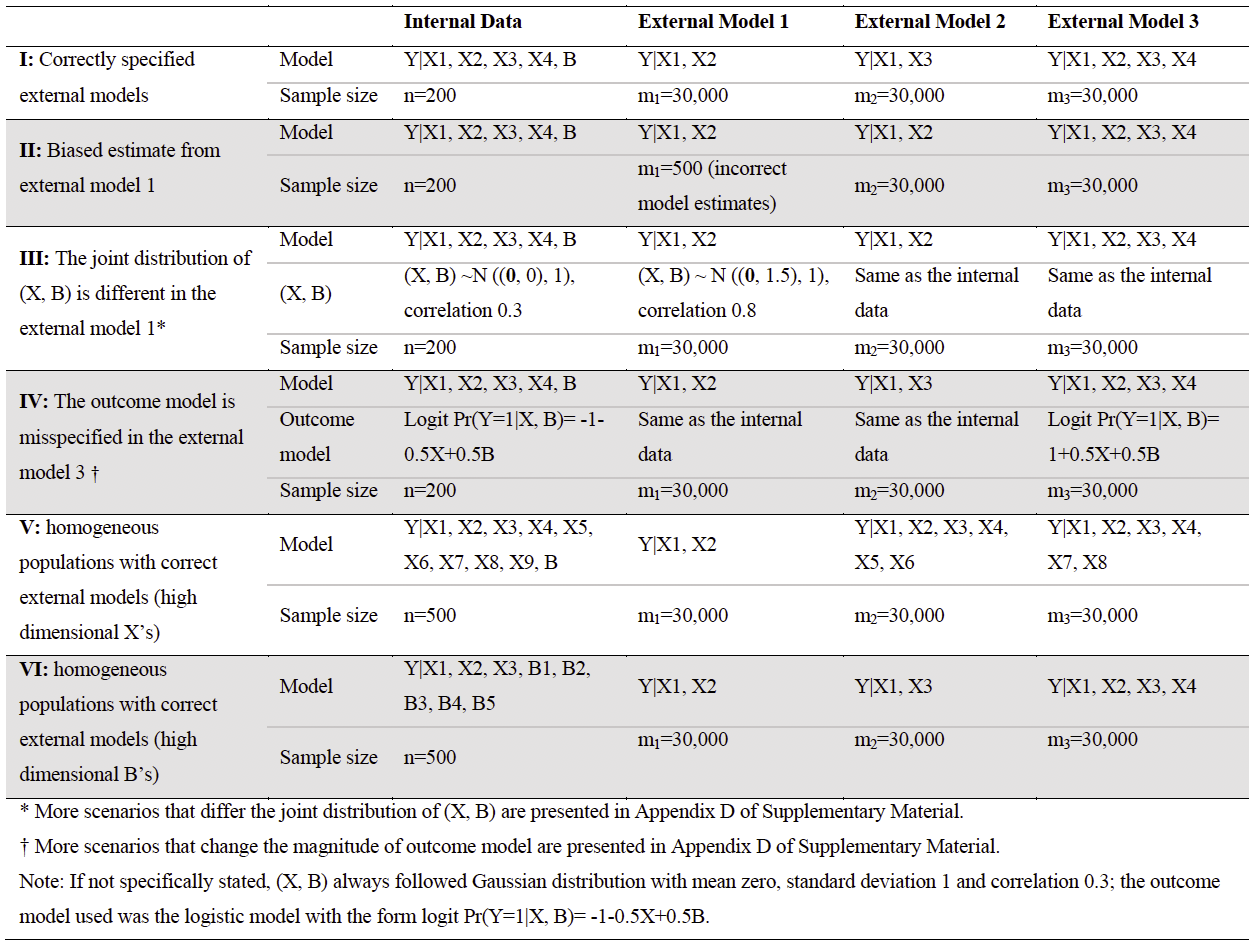
A summary of all the simulation settings is listed in Figure 1. In the first four simulation scenarios (I, II, III, IV), we assumed that a logistic regression model with the following form could describe the relationship among a binary outcome Y and five covariates ($\rm X_{1},X_{2},X_{3},X_{4},B$), where $\rm X_{1},X_{2},X_{3},X_{4}$ had been used in at least one external model while $\rm B$ was only available in the current study: $\rm logit[Pr(Y=1|X_{1},X_{2},X_{3},X_{4},B)]=-1-0.5\sum_{i=1}^{4}X_{i}+0.5B$. Here $\rm X_{1},X_{2},X_{3},X_{4}$ and $\rm B$ followed a standard multivariate normal distribution with 0.3 correlation and the prevalence of $\rm Y=1$ was 0.32.

• •

  Simulation I evaluated the idealized case where the internal and the external models were fitted on the homogeneous population.

• •

  Simulation II assessed the performance of the proposed method when external model 1 had biased $\rm\hat{\boldsymbol{\beta}}$ estimates fitted from $\rm Y|X$, where we obtained the incorrect model estimates by fitting external model 1 on a small dataset of size 500.

• •

  Simulation III aims to show the impact of heterogeneous covariate distribution (X, B) in the external population. As Estes and others 2017 assessed, the disparity of the (X, B) distribution between the two populations can come from (i) a different conditional distribution $\rm B|X$, (ii) a different marginal B distribution, (iii) a different marginal X distribution, or a combination of these reasons. In this simulation scenario, we showed the combination of (i) and (ii) as an example, but we will discuss the result of other scenarios in Simulation Results in Section 3.2.

• •

  Simulation IV evaluated the situation where the outcome model was misspecified in external model 3.

We assumed that there was an internal study of size n=200 and three external models have been fitted to a very large synthetic dataset (sample size $\rm m_{1}=m_{2}=m_{3}=30,000$ for simplicity) that is sampled from the true data generating mechanism and gives precise estimates of the model parameters (except external model 1 in Simulation II). The external sample size need not be as large as 30,000 to achieve good performance as long as the estimated model parameters are close to the true parameters. Sensitivity analysis (results not shown) using external sample size $\rm m_{1}=m_{2}=m_{3}=1,000$ showed small numerical differences compared with m1= m2= m3=30,000.

In simulation V and VI, we considered the outcome model with higher dimension and homogeneous populations between the internal and the external models. In these two scenarios, the internal sample size n=500 was used.

• •

  Simulation V evaluated the situation where the outcome model contained nine X’s and one B: $\rm logit[Pr(Y=1|X_{1},...,X_{9},B)]=-1-0.5\sum_{i=1}^{9}X_{i}+0.5B$. Specifically, the external model 1 only contained two predictors, $\rm X_{1}$ and $\rm X_{2}$, the external model 2 contained seven predictors, $\rm X_{1},...,X_{7}$, and the external model 3 contained six predictors $\rm X_{1},X_{2},X_{3},X_{4},X_{7}$ and $\rm X_{8}$.

• •

  simulation VI evaluated the situation where the full model contained three X’s and five B’s: $\rm logit[Pr(Y=1|X_{1},X_{2},X_{3},B_{1},...,B_{5})]=-1-0.5\sum_{i=1}^{3}X_{i}+0.5\sum_{i=1}^{5}B_{i}$, using the same external models as simulation I.

In Table 1 simulation I, we see that all CML and EB estimators are unbiased as expected. The estimated standard error (ESE, in square brackets) accurately reflect the true standard deviation (SD, in round brackets) from 500 simulations. Both OCWE and SC-Learner had better overall performance than single EB estimators, while SC-Learner outperformed OCWE with respect to both the covariate-wise and the overall metrics (Figure 2).

In Table 1 simulation II, $\rm CML_{1}$ was biased with poor 95% coverage rate due to biased estimation of $\boldsymbol{\hat{\beta}}$. Although trading off most of the precision gain, $\rm EB_{1}$ corrected the bias in $\rm CML_{1}$. The bias of $\rm CML_{1}$ also caused underestimation of the standard error of $\rm EB_{1}$ as highlighted in yellow, which was because $\rm\hat{\boldsymbol{\gamma}}_{CML_{1}}$ differed from $\rm\hat{\boldsymbol{\gamma}_{I}}$ as pointed out in Section 2.4. Despite that, both OCWE and SC-Learner detected the least efficiency gain of $\rm EB_{3}$ among all EB estimators and provided unbiased overall estimates. Moreover, OCWE and SC-Learner had the largest relative efficiency gain compared with the direct regression than other methods, as well as the best performance regarding the relative SSE and Brier Score gain only second to $\rm EB_{3}$ (Figure 2).

Results of simulation III and IV in Table 1 indicates that when incorporating discordant external information from heterogeneous populations (one with different distribution of the joint [X,B] and another with different outcome model), $\rm EB$ estimators are able to correct the bias of $\rm CML$ estimators by trading off some precision-gain, and the proposed estimators could further identify and down-weight that particular $\rm EB$ estimators. Estes and others 2017 provided comprehensive simulation results to show that the EB estimator can protect against the bias due to heterogeneous (X, B) distribution from the external model. Their results indicated that CML estimator would have a substantial bias when the difference came from the conditional distribution $\rm B|X$ or marginal distribution B, and marginal distribution X when the X-B interaction term is involved in the true $\rm Y|X$, B model. When evaluating these scenarios (summary and results in Appendix D in the Supplementary material), we found a similar pattern and conclusion as simulation III. In summary, these simulation results provided the evidence that the proposed approach is robust to the heterogeneous covariate distribution (X, B) of the external population.

In addition to simulation IV, we have assessed different forms of misspecified outcome model in the external population listed in Table D3 from Appendix D of the Supplementary Material, including different intercept only and different X coefficients only, which showed similar conclusions. Simulation IV also showed that although higher dimension of the external model will lead to better overall prediction when the internal and external has the same population (simulation I and II), it is not the case when the transportability assumption is violated: OCWE identified that the external model 3 came from a different distribution than the internal study and thus assigned the smallest weight to $\rm EB_{3}$, even though it had the greatest number of predictors compared with the other two external models. In both simulations, OCWE and SC-Learner had similar covariate-wise and overall performances (Figure 2).

Table 1 (Cont’d) further shows that the proposed estimators have decent performance when the number of predictors in the external models has large differences (simulation V) and when the dimension of B is larger than X’s (simulation VI). In simulation V, compared with other external models that included more than six predictors, the external model 1 only used two predictors and thus provided the least amount of extra information. We see that OCWE assigns the minimum weight to $\rm EB_{1}$ and achieves the largest relative efficiency gain among all estimators (Figure 3). The fact that SC-Learner outperformed OCWE with respect to decreasing the covariate-wise variance of $\rm\hat{\gamma}_{5}$ to $\rm\hat{\gamma}_{9}$ reveals that SC-Learner is flexible enough to select the external information on the covariate-level when $\rm p_{k}$ (the number of predictors used in the $\rm k^{th}$ external model) is very different from others. Simulation VI showed that when the dimension of B was much larger than X, the overall benefit of combining multiple EB estimators would be limited due to the small amount of external information added from the external models.

References

- Bareinboim and Pearl (2013) Bareinboim, E. and Pearl, J. (2013). A general algorithm for deciding transportability of experimental results. Journal of Causal Inference 1, 107–134.
- Bohnen and others (2007) Bohnen, A.M., Groeneveld, F.P. and Bosch, J.L.H.R. (2007). Serum prostate-specific antigen as a predictor of prostate volume in the community: the krimpen study. European Urology 51, 1645–1653.
- Breiman (1996) Breiman, L. (1996). Bagging predictors. Machine Learning 24, 123–140.
- Breiman (2001) Breiman, L. (2001). Bagging predictors. Random forests 45, 5–32.
- (5) Bycroft, C. Integrated household surveys: A survey vehicles approach. Wellington: Statistics New Zealand.
- Chatterjee and others (2016) Chatterjee, N., Chen, Y.-H., P.Maas and Carroll, R. J. (2016). Constrained maximum likelihood estimation for model calibration using summary-level information from external big data sources. Journal of the American Statistical Association 111, 107–117.
- Cheng and others (2019) Cheng, W., Taylor, J.M.G., Tomlins, T. and Mukherjee, B. (2019). Informing a risk prediction model for binary outcomes with external coefficient information. Journal of the Royal Statistical Society: Series C (Applied Statistics) 68, 121–139.
- Cheng and others (2018) Cheng, W., Taylor, J.M.G., Vokonas, P.S., Park, S.K. and Mukherjee, B. (2018). Improving estimation and prediction in linear regression incorporating external information from an established reduced model. Statistics in Medicine 37, 1515–1530.
- Dejardin and others (2018) Dejardin, D., Delmar, P., Warne, C., Patel, K., van Rosmalen, J. and Lesaffre, E. (2018). Use of a historical control group in a noninferiority trial assessing a new antibacterial treatment: A case study and discussion of practical implementation aspects. Pharmaceutical Statistics 17, 169–181.
- Estes and others (2017) Estes, J.P., Mukherjee, B. and Taylor, J.M.G. (2017). Empirical bayes estimation and prediction using summary-level information from external big data sources adjusting for violations of transportability. Statistics in Biosciences 10, 568–586.
- Freund and Schapire (1997) Freund, Y. and Schapire, R.R. (1997). A decision-theoretic generalization of on-line learning and an application to boosting. Journal of Computer and System Sciences 55, 119–139.
- Gail and others (1989) Gail, M. H., Brinton, L. A., Byar, D. P., Corle, D. K., Green, S. B., Schairer, C. and Mulvihill, J. J. (1989). Projecting individualized probabilities of developing breast cancer for white females who are being examined annually. Journal of the National Cancer Institute 81, 1879–1886.
- Goos and Jones (2011) Goos, P. and Jones, B. (2011). Optimal Design of Experiments: A Case Study Approach. Wiley.
- Gu and others (2019) Gu, T., Taylor, J.M.G. and Mukherjee, B. (2019). Synthetic data method to incorporate external information into a current study. Canadian Journal of Statistics 47, 580–603.
- Han and Lawless (2019) Han, P. and Lawless, J.F. (2019). Empirical likelihood estimation using auxiliary summary information with different covariate distribution. Statistics Sinica 29, 1321–1342.
- Kundu and others (2019) Kundu, P., Tang, R. and Chatterjee, N. (2019). Generalized meta-analysis for multiple regression models across studies with disparate covariate information. Biometrika 106, 567–585.
- Li and Song (2020) Li, X. H. and Song, Y. (2020). Target population statistical inference with data integration across multiple sources—an approach to mitigate information shortage in rare disease clinical trials. Statistics in Biopharmaceutical Research 12, 322–333.
- Qin (2000) Qin, J. (2000). Combining parametric and empirical likelihoods. Biometrika 87, 484–90.
- Roobol and others (2012) Roobol, M.J., van Vugt, H.A., Loeb, S., Zhu, X., Bul, M., Bangma, C. H., van Leenders, A. G., Steyerberg, E. W. and Schröder, F. H. (2012). Prediction of prostate cancer risk: the role of prostate volume and digital rectal examination in the ERSPC risk calculators. European Urology 61, 577–583.
- Schapire (1990) Schapire, R.E. (1990). The strength of weak learnability. Machine Learning 5, 197–227.
- Simpkin and others (2016) Simpkin, A. J., Donovan, J.L., Tilling, K., Lane, J. Athene, Martin, R. M., Albertsen, P.C., Bill-Axelson, A., Carter, H. Ballentine, Bosch, J.L., Ferrucci, L., Hamdy, F.C., Holmberg, L., Metter, E. Jeffrey, Neal, D.E., Parker, C.C. and others. (2016). Prostate-specific antigen patterns in us and european populations: comparison of six diverse cohorts. BJU International 118, 911–918.
- van der Laan and others (2007) van der Laan, M.J., Polley, E.C. and Hubbard, A.E. (2007). Super learner. Statistical Applications in Genetics and Molecular Biology 6.
- Thompson and others (2006) Thompson, I. M., Ankerst, D. P., Chi, C., Goodman, P. J., Tangen, C. M., Lucia, M. S., Feng, Z., Parnes, H. L. and Coltman, C. A. (2006). Assessing prostate cancer risk: Results from the prostate cancer prevention trial. European Urology 98, 529–534.
- Tomlins and others (2015) Tomlins, S. A., Day, J. R., Lonigro, R. J., Hovelson, D. H., Siddiqui, J., Kunju, L. P., Dunn, R. L., Meyer, S., Hodge, P., Groskopf, J., Wei, J. T. and others. (2015). Urine TMPRSS2:ERG plus PCA3 for individualized prostate cancer risk assessment. European Urology 70, 45–53.
- Truong and others (2013) Truong, M., Yang, B. and Jarrard, D. F. (2013). Toward the detection of prostate cancer in urine: a critical analysis. Journal of Urology 189, 422–429.
- Viele and others (2014) Viele, K., Berry, S., Neuenschwander, B., Amzal, B., Chen, F., Enas, N., Hobbs, B., Ibrahim, J.G., Kinnersley, N. and et al., S. Lindborg. (2014). Use of historical control data for assessing treatment effects in clinical trials. Pharmaceutical Statistics 13, 41–54.
- Yang and Ding (2020) Yang, S. and Ding, P. (2020). Combining multiple observational data sources to estimate causal effects. Journal of the American Statistical Association 3, 1540–1554.
- Yang and Kim (2020) Yang, S. and Kim, J.K. (2020). Statistical data integration in survey sampling: a review. Japanese Journal of Statistics and Data Science 3, 625–650.
- Zhang and others (2020) Zhang, H., Deng, L., Schiffman, M., Qin, J. and Yu, K. (2020). Generalized integration model for improved statistical inference by leveraging external summary data. Biometrika 107, 689–703.
Simulation Direct Regression Internal Data + External 1 Internal Data + External 2 Internal Data + External 3 Composite of EB Estimators CML 1 EB 1 CML 2 EB 2 CML 3 EB 3 IVW OCWE SC-Learner Bias (SD) [ESE] 95% Coverage Rate I Weight / / / / / / / (.33, .33,.33) (.27, .12, .61) / -.041 (.197) [.193] -.008 (.081) [.085] -.032 (.162) [.160] -.007 (.089) [.084] -.032 (.163) [.161] .004 (.050) [.085] -.033 (.169) [.168] -.032 (.164) [.162] -.031 (.166) [.164] -.032 (.164) [.162] 95% 96% 95% 95% 95% 98% 95% 95% 95% 95% -.020 (.229) [.208] -.004 (.095) [.097] -.014 (.190) [.173] -.002 (.089) [.097] -.013 (.188) [.174] -.002 (.066) [.074] -.016 (.198) [.181] -.014 (.191) [.176] -.016 (.194) [.178] -.014 (.191) [.175] 94% 96% 93% 97% 93% 96% 93% 93% 93% 93% -.017 (.219) [.208] -.008 (.091) [.096] -.014 (.180) [.173] -.003 (.062) [.210] -.014 (.188) [.182] -.015 (.195) [.187] -.011 (.190) [.181] -.014 (.184) [.176] 94% 97% 94% 97% 94% 94% 94% 94% -.018 (.208) [.207] -.002 (.090) [.095] -.013 (.171) [.174] -.002 (.062) [.174] -.015 (.177) [.182] -.015 (.185) [.185] -.012 (.184) [.186] -.014(.174) [.176] 96% 98% 96% 96% 95% 95% 95% 95% -.026 (.217) [.208] -.007 (.067) [.208] -.022 (.187) [.194] -.025 (.207) [.196] -.023 (.198) [.191] -.022 (.187) [.194] 94% 97% 96% 94% 95% 96% .016 (.219) [.207] II Weight / / / / / / / [.33, .33, .34] [.23, .28, .49] / -.042 (.198) [.193] .042 (.080) [.086] -.024 (.168) [.161] -.008 (.081) [.085] -.032 (.162) [.160] .003 (.050) [.058] -.034 (.170) [.169] -.031 (.166) [.162] -.031 (.167) [.163] -.031 (.166) [.162] 95% 87% 94% 96% 95% 98% 95% 95% 95% 95% -.020 (.229) [.208] .153 (.094) [.100] -.015 (.202) [.174] -.004 (.095) [.097] -.014 (.190) [.173] -.017 (.066) [.074] -.018 (.198) [.182] -.007 (.196) [.176] -.009 (.197) [.177] -.007 (.196) [.175] 94% 65% 92% 96% 93% 97% 94% 93% 92% 93% -.018 (.220) [.208] -.143 (.091) [.098] -.041 (.190) [.174] -.008 (.091) [.096] -.014 (.180) [.173] .009 (.062) [.073] -.013 (.188) [.183] -.022 (.185) [.176] -.020 (.186) [.177] -.028 (.189) [.177] 94% 70% 93% 96% 94% 95% 94% 94% 94% 94% -.019 (.208) [.207] .015 (.062) [.072] -.012 (.178) [.194] -.016 (.198) [.195] -.015 (.193) [.192] -.015 (.192) [.192] 96% 94% 97% 95% 95% 95% -.027 (.217) [.208] .004 (.067) [.073] -.021 (.187) [.195] -.025 (.207) [196] -.021 (.202) [.193] -.021 (.187) [.195] 94% 97% 96% 94% 94% 96% -.017 (.219) [.207] 98% III Weight / / / / / / / [.33, .33, .33] [.15, .35, .49] / -.041 (.198) [.193] .648 (.082) [.100] -.009 (.199) [.162] -.039 (.081) [.085] -.004 (.162) [.160] -.033 (.051) [.058] -.039 (.169) [.168] -.029 (.176) [.163] -.031 (.173) [.163] -.029 (.176) [.162] 95% 0% 91% 97% 95% 98% 95% 93% 93% 93% -.019 (.228) [.208] -.156 (.096) [.113] -.026 (.221) [.175] .012 (.095) [.097] -.010 (.189) [.173] .022 (.066) [.074] -.012 (.197) [.181] -.016 (.202) [.176] -.014 (.198) [.177] -.016 (.202) [.176] 94% 75% 89% 97% 93% 97% 94% 91% 93% 91% -.017 (.219) [.208] .160 (.091) [.113] -.024 (.211) [.175] -.015 (.091) [.096] -.015 (.179) [.173] -.005 (.062) [.073] -.014 (.188) [.182] -.017 (.192) [.176] -.016 (.188) [.177] -.019 (.200) [.177] 95% 76% 90% 97% 94% 95% 94% 93% 94% 93% -.019 (.209) [.207] -.014 (.062) [.072] -.014 (.178) [.182] -.018 (.198) [.195] -.017 (.193) [.192] -.018 (.192) [.192] 96% 94% 97% 96% 94% 96% -.026 (.217) [.208] -.021 (.067) [.073] -.021 (.188) [.194] -.026 (.207) [.196] -.025 (.202) [.193] -.025 (.188) [.195] 94% 97% 96% 94% 95% 96% .017 (.219) [.207] 98% IV Weight / / / / / / / [.34, .33, .32] [.57, .38,.04] / -.041 (.198) [.193] -.008 (.081) [.085] -.032 (.163) [.161] -.007 (.089) [.084] -.032 (.164) [.161] 1.69 (.189) [.162] -.031 (.169) [.178] -.032 (.173) [.165] -.030 (.164) [.160] -.032 (.172) [.164] 95% 96% 94% 95% 95% 0% 96% 93% 93% 93% -.020 (.230) [.208] -.005 (.095) [.097] -.014 (.190) [.174] -.002 (.089) [.097] -.014 (.189) [.174] .747 (.178) [.177] -.016 (.197) [.192] -.015 (.201) [.178] -.013 (.191) [.173] -.015 (.200) [.178] 94% 96% 93% 97% 93% 3% 95% 92% 93% 92% -.018 (.220) [.208] -.008 (.091) [.096] -.014 (.180) [.175] .756 (.174) [.177] -.014 (.188) [.192] -.015 (.206) [.189] -.013 (.196) [.187] -.014 (.197) [.177] 95% 97% 94% 3% 94% 93% 94% 93% -.019 (.208) [.207] -.003 (.089) [.095] -.013 (.171) [.180] .762 (.167) [.175] -.014 (.178) [.191] -.015 (.194) [.187] -.013 (.193) [.189] -.014 (.187) [.181] 96% 98% 96% 1% 95% 95% 94% 95% -.026 (.216) [.208] .746 (.179) [.176] -.022 (.188) [.193] -.025 (.216) [.202] -.026 (.217) [.207] -.022 (.216) [.193] 94% 4% 93% 94% 95% 94% .019 (.218) [.207] 98%
Simulation Direct Regression Internal Data + External 1 Internal Data + External 2 Internal Data + External 3 Composite of EB Estimators CML 1 EB 1 CML 2 EB 2 CML 3 EB 3 IVW OCWE SC-Learner Bias (SD) [ESE] 95% Coverage Rate V Weight / / / / / / / (.33, .33,.33) (.13, .432, .429) / -.035 (.153) [.149] .02 (.100) [.098] .031 (.132) [.129] -.002 (.054) [.059] -.031 (.139) [.137] -.010 (.064) [.066] -.031 (.137) [.135] -.031 (.135) [.132] -.031 (.137) [.133] -.031 (.135) [.132] 94% 95% 95% 97% 94% 96% 94% 94% 94% 94% -.023 (.160) [.158] .002 (.089) [.094] .016 (.133) [.133] .010 (.055) [.061] -.019 (.144) [.144] .009 (.061) [.067] -.019 (.142) [.142] -.018 (.139) [.139] -.019 (.141) [.141] -.018 (.139) [.139] 94% 96% 94% 97% 94% 97% 94% 94% 94% 94% -.027 (.153) [.158] .014 (.094) [.094] .023 (.128) [.133] -.006 (.056) [.060] -.024 (.137) [.144] .013 (.064) [.066] -.025 (.136) [.142] -.024 (.133) [.139] -.024 (.135) [.141] -.024 (.133) [.138] 95% 95% 95% 97% 94% 96% 95% 95% 95% 95% -.037 (.161) [.158] .002 (.057) [.061] -.031 (.144) [.145] .002 (.064) [.067] -.031 (.143) [.143] -.033 (.149) [.148] -.031 (.145) [.145] -.031 (.143) [.143] 95% 97% 95% 97% 95% 95% 95% 95% -.014 (.162) [.157] .025 (.054) [.060] -.014 (.145) [.144] .025 (.062) [.066] -.016 (.144) [.142] -.015 (.150) [.147] -.014 (.147) [.144] -.015 (.145) [.142] 94% 97% 95% 96% 95% 95% 95% 96% -.014 (.160) [.158] .010 (.055) [.060] -.011 (.143) [.153] -.013 (.154) [.150] -.012 (.153) [.150] -.011 (.143) [.153] 96% 97% 95% 95% 95% 96% -.023 (.160) [.158] -.010 (.057) [.061] -.021 (.143) [.153] -.023 (.154) [.151] -.022 (.152) [.151] -.021 (.143) [.153] 95% 99% 96% 95% 95% 96% -.015 (.165) [.158] -.008 (.056) [.060] -.014 (.148) [.153] -.015 (.159) [.150] -.015 (.157) [.150] -.014 (.148) [.153] 95% 99% 96% 95% 95% 96% -.033 (.159) [.159] -.001 (.063) [.067] -.029 (.141) [.151] -.031 (.153) [.152] -.031 (.151) [.151] -.029 (.141) [.151] 95% 98% 96% 97% 95% 97% -.027 (.154) [.154] -.021 (.066) [.067] -.026 (.136) [.151] -.026 (.148) [.151] -.026 (.146) [.150] -.026 (.136) [.151] 97% 97% 97% 97% 95% 97% .034 (.172) [.172] 97% VI Weight / / / / / / / [.33, .33, .34] [.01, .0004, .987] / -.027 (.126) [.121] .003 (.078) [.073] -.020 (.108) [.103] .003 (.078) [.073] -.031 (.108) [.103] .005 (.078) [.073] -.020 (.110) [.105] -.020 (.109) [.104] -.020 (.110) [.105] -.020 (.109) [.104] 94% 92% 94% 93% 94% 92% 94% 94% 94% 94% -.012 (.132) [.132] -.015 (.088) [.085] -.013 (.115) [.115] -.019 (.086) [.085] -.019 (.115) [.115] -.019 (.084) [.081] -.013 (.116) [.116] -.013 (.115) [.115] -.013 (.116) [.116] -.013 (.115) [.115] 95% 95% 95% 94% 95% 95% 95% 95% 95% 95% -.004 (.137) [.132] .005 (.087) [.085] .004 (.118) [.115] .004 (.084) [.081] .003 (.119) [.117] .004 (.124) [.121] .003 (.119) [.117] .004 (.118) [.116] 93% 95% 93% 94% 94% 93% 94% 94% -.011 (.131) [.132] .005 (.085) [.085] -.007 (.113) [.117] .005 (.081) [.082] -.007 (.114) [.118] -.008 (.119) [.121] -.007 (.114) [.118] -.007 (.113) [.117] 96% 95% 96% 94% 96% 96% 96% 96% .007 (.126) [.121] 95% -.025 (.137) [.132] 96% -.014 (.135) [.132] 97% -.012 (.131) [.132] 96% -.013 (.139) [.132] 95%
Direct Regression PCPThg ERSPC Internal data + PCPThg Internal data + ERSPC Composite of EB Estimators Original Estimated Original Estimated CML 1 EB1 CML 2 EB2 IVW OCWE SC-Learner Weight / / / / / / / / / [.5, .5] [.99, .00] / .1199 / .065 / .048 .073 .104 .078 .105 .104 ( 13.2%) .104 ( 13.2%) .0996 ( 17.2%) Brier Score .902 1.059 .987 .954 .994 .942 .901 .847 .901 .901 ( .12%) .901 ( .12%) .901 ( .12%) Point estimate (ESE) % ESE w.r.t direct regression Intercept -4.123 (.449) -3.686268 -1.395 (.115) -3.16 -1.382 (.111) -6.422 (.437) -4.128 (.445) -5.989 (.437) -4.130 (.444) -4.129 (.443) -4.128 (.445) -4.129 (.443) REF / 74% / 75% 3% 1% 3% 1% 1% 1% 1% (PSA) 0.860 (.144) 0.8941599 0.721 (.123) 1.175573 .878 (.123) 0.893 (.103) 0.860 (.132) 1.159 (.081) 0.861 (.124) 0.860 (.127) 0.860 (.130) 0.860 (.127) REF / 14% / 14% 28% 8% 44% 14% 11% 9% 12% DRE 1.028 (.297) 1 1.134 (.256) 1.813195 1.298 (.269) 0.687 (.218) 1.027 (.269) 1.430 (.170) 1.029 (.253) 1.028 (.259) 1.027 (.269) 1.028 (.258) REF / 14% / 9% 26% 9% 43% 15% 13% 9% 13% Age 0.0315 (.014) 0.03 0.0328 (.012) 0.0304 (.009) 0.0315 (.013) 0.032 (.014) 0.031 (.014) 0.032 (.014) 0.032 (.013) 0.032 (.013) REF / 14% 31% 8% 1% 8% 8% Biopsy -1.165 (.290) -0.36 -1.413 (.270) -0.0286 (.158) -1.163 (.255) -1.187 (.290) -1.165 (.291) -1.164 (.272) -1.163 (.255) -1.163 (.255) REF / 7% 46% 12% 6% 12% 12% Race 0.193 (.329) 0.96 0.448 (.287) 0.819 (.218) 0.194 (.291) 0.160 (.329) 0.193 (.329) 0.193 (.308) 0.194 (.291) 0.194 (.291) REF / 13% 34% 12% 6% 12% 12% (TRUS-PV) -1.663 (.252) -1.514128 -1.681 (.224) -1.683 (.252) -1.663 (.252) -1.491 (.155) -1.663 (.223) -1.663 (.236) -1.663 (.252) -1.663 (.223) REF / 11% 38% 12% 6% 0% 12% (PCA3+1) .485 (.088) 0.495 (.088) 0.485 (.088) 0.507 (.088) 0.485 (.088) 0.485 (.088) 0.485 (.088) 0.486 (.088) REF (T2:ERG+1) .096 (.037) 0.095 (.037) 0.096 (.037) 0.099 (.037) 0.096 (.037) 0.096 (.037) 0.096 (.037) 0.096 (.037) REF