Improvements to Pan-STARRS1 Astrometry Using GaiaJournal: AJ
Abstract
We use the Gaia DR2 catalog to improve the astrometric accuracy of about 1.7 billion objects in Pan-STARRS1 Data Release 2 (PS1 DR2). We also obtain proper motions for these PS1 objects. The cross match between Gaia and PS1 reveals residuals that are correlated on a scale of about 1 arcmin. We apply a spatially adaptive correction algorithm for all PS1 objects having more than two detections to reduce these residuals and align the object positions to Gaia. For point-like PS1 objects that cross match to Gaia, the algorithm reduces PS1/Gaia residuals by 33% in position (median value of 13.5 mas reduced to 9.0 mas) and by 24% in proper motion (median value of 6.3 mas/yr reduced to 4.8 mas/yr). The residuals for the corrected positions are smallest for objects with the most point-like morphologies and with intermediate magnitudes of about 17 mag. The residual errors in declination are systematically larger than those in right ascension; the declination errors increase with zenith angle in proportion to the air mass of the observations. Declination positional residuals at a given declination generally vary with color and are consistent with the effects of differential atmospheric refraction. In principle, these residuals could be reduced further by taking into account object color.
Keywords:
Surveys:Pan-STARRS1; astrometry; catalogs; proper motions; Astrophysics - Instrumentation and Methods for AstrophysicsI Introduction
The Panoramic Survey Telescope and Rapid Response System (Pan-STARRS) has carried out a 3 steradian survey of the sky, north of declination degrees. The Pan-STARRS1 survey (PS1) was carried out mainly from 2010 to 2014 at Haleakala Observatory in Hawaii by covering the sky region about 12 times in each of five broadband filters (, , , , ). Several papers are available that describe the system design, pipeline, calibration, and results; Chambers et al. 2016 provides an overview. There have been two data releases, DR1 and DR2. DR1 (2016 December) contained only average information resulting from individual exposures. The second data release, DR2 (2019 January), contains time-dependent information obtained from individual exposures. In this paper we make use of DR2.11 1 When we refer to PS1 data products, we mean the DR2 versions unless we explicitly mention DR1.
PS1 DR2 contains over 1.6 petabytes of data including measurements for more than 10 billion objects, making it the largest volume of astronomical information released to date. The image data and an object catalog are made available online at http://panstarrs.stsci.edu through the Barbara A. Mikulski Archive for Space Telescopes (MAST) at the Space Telescope Science Institute. The catalog consists of tables that are stored in Microsoft SQL Server databases (Flewelling et al. 2016). The PS1 catalog database makes use of software previously developed for SDSS on SQL Server (Thakar et al. 2003; Heasley 2008). The tables can be accessed through a web form and Application Programming Interface (API) at https://catalogs.mast.stsci.edu or through an SQL query interface called CasJobs at https://mastweb.stsci.edu/ps1casjobs. It is also accessible via a Virtual Observatory Table Access Protocol22 2 http://ivoa.net/documents/TAP (TAP) interface at http://vao.stsci.edu/PS1DR2/tapservice.aspx.
In this paper we are concerned with improving the astrometry of the PS1 DR2 catalog. There are several motivations to improve the PS1 astrometry. Although the Gaia catalog (Lindegren et al. 2018) provides more accurate astrometry than PS1, PS1 reaches fainter objects (mag 23) than Gaia (mag 20). For this reason, PS1 astrometry can play an important role. For example, for the purposes of determining the astrometry of images taken by the Hubble Space Telescope, we have found in the construction of the Hubble Source Catalog (Whitmore et al. 2016) that about 20% to 30% of the images taken with the wide field instruments (the Wide Field and Planetary Camera 2, Advanced Camera for Surveys, and Wide Field Camera 3) do not contain enough unsaturated stars in common with Gaia to provide an astrometric solution. This situation is of importance for high Galactic latitude fields where the density of stars is relatively low. The James Webb Space Telescope (JWST) will have similar issues, with the added complication that even faint Gaia stars will often be saturated in JWST images. In such cases, PS1 provides an important alternative astrometric reference catalog having higher source density and fainter objects.
The astrometric calibration of the current PS1 DR2 catalog is described in Magnier et al. 2016. The astrometry was calibrated using 2MASS (Skrutskie et al. 2006) and Gaia DR1 (Lindegren et al. 2016) object positions that were available at the time of the PS1 data processing. The Gaia positions were much more heavily weighted in the PS1 astrometric determinations due to their much smaller errors. A major issue in this calibration procedure is the presence of systematic proper motions that lead to nonrandom shifts between PS1 stellar positions and those in 2MASS and Gaia. Gaia DR1 does not provide proper motions. These proper motions were modeled in PS1 by using by a flat rotation curve for the Galactic disk. Making these proper motion corrections for each cross-matched disk object requires a knowledge of the distance to the object that is estimated by its distance modulus. As discussed by Magnier et al. 2016, this process and other issues introduce some astrometric uncertainties. In this paper we utilize the Gaia DR2 positions, proper motions, and parallaxes to improve the PS1 astrometry.
In comparing Gaia and PS1 object positions, we find small scale arcmin structures in the residuals. To mitigate against such effects, we employ an adaptive astrometric correction algorithm that smooths and reduces residuals on that scale.
In this paper we describe the determination for the first time of proper motions for PS1 objects. We describe the correction algorithm for improving the astrometric accuracy of PS1 by making use of Gaia DR2 and analyze the results. We also apply a similar correction procedure to improve the PS1 proper motion accuracy by making use of the proper motions available in Gaia DR2. These improvements will be integrated into the MAST PS1 catalog.
The outline of this paper is as follows. In Section II we provide some background for our calculations by describing the mean object positions and proper motions that we utilize as inputs to our correction algorithm. We also provide some examples of the PS1/Gaia residuals that we aim to correct. Section III describes our correction algorithm. Section IV describes the PS1 positional and proper motion residuals of reference objects (high quality detections that cross match to Gaia) that occur over the entire PS1 sky region before and after the corrections we apply. In Section V we describe how the number of the objects varies with declination. We then discuss how the position residuals of reference objects vary with declination (Section VI) and color (Section VII). Section VIII describes the variations of proper motion residuals with declination. Section IX describes some additional checks on the results, including comparisons to the Hubble Source Catalog and the ICRF2 radio catalog (Ma et al. 2009) to explore the PS1 astrometric accuracy at faint magnitudes. Section X contains the discussion and summary. The convergence of the positional correction shifts is discussed in Appendix A.
II Background
The PS1 database tables contain positional and photometric information about the detected objects. The database contents are described in detail in Flewelling et al. 2016 and in the PS1 archive documentation (https://panstarrs.stsci.edu). Positional information based on individual single-epoch exposures is available in the Detection table (actually, a view or virtual table). Stack images are creating by combining all the single-epoch exposures in a given filter to get a deeper image. Table StackObjectThin contains positional information on each object for each filter as determined from the stack images. The ObjectThin table contains summary information from both the single-epoch measurements and the stack measurements in the form of weighted means of the values measured at different epochs and filters.
II.1 Computation of Mean Positions
It might appear natural to recalibrate the astrometry starting from the weighted positions (raMean and decMean) in the ObjectThin table. However, that is not possible because those positions are contaminated by Gaia DR1 data for objects that match Gaia. In PS1 DR1 and DR2, cross-matched Gaia positions are included with high weighting in the determination of mean PS1 positions (Magnier et al. 2016). The combined positions are weighted by the inverse variances of the position measurements; since the Gaia errors are much smaller than the PS1 errors, the effect is that the database positions for PS1 objects that match Gaia are almost equal to the Gaia DR1 measurements. A comparison of Gaia and PS1 DR2 positions for the objects in common yields a typical residual of about 5 mas. While those positions are in fact very accurate, they derive that accuracy not from the PS1 measurements but from Gaia. The excellent agreement between PS1 database positions and Gaia positions is not an independent measurement of the PS1 positional accuracy, and the PS1/Gaia differences do not reflect the typical PS1 astrometric errors for the large majority of PS1 objects that do not match Gaia. Makarov et al. 2017 carried out an independent assessment of PS1 astrometry using 19 million Gaia stars that were excluded from the PS1 astrometric calibration due to their Gaia catalog flags. They found that the residual systematic uncertainties for the PS1 positions are closer to 20 mas. Note that the Makarov et al. 2017 paper relied on an earlier astrometric calibration of PS1 (PV3.2) that was affected by a poor quality astrometric flag-field correction. That correction was repaired in PS1 DR2 (Magnier et al. 2016).
Rather that use the positions from ObjectThin, we compute new mean positions and proper motions directly from the single-epoch PS1 positions in the Detection table. The values in the Detection table do not include Gaia DR1 data (although they were calibrated using that data). We restrict our sample to objects that have good measurements for at least three epochs. We exclude measurements having infoFlag3 bit 16 set (indicating the measurement was an astrometric outlier) and also exclude detections having a psfQfPerfect value less than 0.9 (indicating that there are bad pixels within the core of the stellar image). The full PS1 ObjectThin contains entries for about 10 billion objects. After excluding objects with fewer than three good measurements, we are left with approximately 1.7 billion objects. Those objects are the topic of this paper.
Note that the astrometric correction algorithm described in this paper also relies on the PS1/Gaia cross-match. However, for each PS1 object, we explicitly exclude the Gaia match for that object (if there is one); we compute the correction using only the offsets from nearby objects. As a result, the positions in our catalog are in the Gaia reference frame but are not biased by the inclusion of Gaia data. Our new PS1 positions are independent measurements that are not correlated with Gaia DR2 measurements of the same stars.
II.2 Selection of Point-like Reference Objects Using ps-score
Using a machine learning model, Tachibana & Miller 2018 classified about 1.5 billion objects from the PS1 DR1 as either extended objects (resolved) or point sources (unresolved). Objects were ranked probabilistically by a quantity called the point-source score (hereafter ps-score) on a scale in which 0 represents extended objects and 1 represents point sources. The results of this analysis are provided as a MAST high level product (see https://archive.stsci.edu/prepds/ps1-psc/) and as a CasJobs table in context HLSP_PS1_PSC.
In this paper, we make use of ps-score values in several ways. We restrict the sample of PS1/Gaia matches used for the calibration to PS1 objects having high ps-score values, which improves the accuracy of the results (particularly in crowded fields where many PS1 objects are blended). We also use the ps-score values to select sources for assessing the accuracy of our corrected astrometry. Our justifications for this approach are discussed below (Section IV).
However, we are using PS1 DR2 rather than DR1 for which ps-score values were obtained. PS1 identifies objects with a unique identifier called objid. The ps-scores are associated with an objid in DR1. Most of the objects in PS1 DR1 are carried over with the same objid in DR2, although some DR2 objects do not have a ps-score value. We have found that less than about 10% of the DR2 objects are missing ps-scores in low density regions. The percentage is higher in high density regions such as the Galactic plane. But since there are many PS1 and Gaia sources available in such regions, our analysis is not much affected by these missing scores. Consequently, we are able to make use of the PS1 DR1 ps-score values for certain aspects of our calculations.
Note that we calculate improved astrometry for all 1.7 billion objects selected as described in Section II.1, regardless of their ps-score values. The restriction of our sample using the ps-score values applies only to selecting objects for the positional calibration and for assessing of the results.
II.3 Astrometric Errors in the PS1 DR2 Catalog
Figures 1 and 2 illustrate the systematic astrometric errors that are corrected in this paper. The left panel in Figure 1 shows the offsets between our PS1 mean positions and Gaia DR2 positions as a function of position in a typical PS1 field. The Gaia positions have been shifted using the Gaia proper motions to the epoch of the corresponding PS1 object. (The epoch is different for every object due to the complex grid of overlapping exposures.) Systematic distortions of up to tens of milliarcseconds are apparent on scales of one to a few arcminutes. After correction using the algorithm described below, the systematic errors are greatly reduced (right panel).
We are not certain what causes the astrometric errors on the arcmin scale that we correct. The astrometric calibration carried out by Magnier et al. 2016 involves making global corrections involving at most cubic polynomials on the chip scale. Since the chip size is 20 arcmin on each edge, this provides independent corrections on the larger arcmin scale. That is a likely contributor to the corrected errors.
Figure 2 shows the distribution of positional errors before and after our correction for all the objects in this field. This field was selected as a typical example of the improvement found throughout the PS1 survey area. The pattern and amplitude of the distortions varies from field to field, but qualitatively similar distortions are found in all fields. Removing the systematic, spatially correlated distortions results in substantial improvements to the overall accuracy of the PS1 astrometry. The algorithm used to achieve this improvement is described in the next section.
III Correction Algorithm
III.1 Mean Detection Positions
The initial step in calculating new positions is to combine the positions measured at every epoch (from the Detection table) to get a new “mean detection” position for every object. As was mentioned above, the infoFlag3 and psfQfPerfect fields are used to exclude poor quality measurements, and only objects with at least three good measurements are included. The Detection table’s ra and dec values are combined using weighting from the errors raErr and decErr to get the weighted mean position. The PMs in RA and declination are also determined using a weighted linear fit to the positions as a function of the observing epoch obsTime. The result of the fit is a new table of PS1 DR2 positions uncontaminated by the Gaia DR1 measurements (mdra, mddec), along with the PMs (mdpmra, mdpmdec). Simple propagation of errors is used to calculate the errors on these quantitites (mdraErr, mddecErr, mdpmraErr, mdpmdecErr). The weighted mean observation epochs (mdmjdra, mdmjddec) are used as the reference time for the fits so that the covariances between the positions and PMs are formally zero. The values of the fits to the data are also computed (chisqra, chisqdec).
III.2 Astrometric Distortion Correction
We correct the systematic distortions between PS1 coordinates and Gaia coordinates (Fig. 1) using the shifts of nearby PS1 objects that cross match to Gaia, objects that we call reference objects. In doing so, we are assuming that these reference shifts vary smoothly with position on the scale of the distance between the reference objects. This local shift can be computed regardless of whether a particular PS1 object has a Gaia counterpart or not. (Most PS1 objects do not have a match in Gaia.)
We experimented with several different algorithms for choosing the cohort of nearby reference objects (referred to as the neighborhood) for correcting the astrometry. An algorithm using objects out to some fixed radius works well as long as there are enough close object, but it can fail either when the radius is too small (leading to too few reference objects and a noisy correction) or when the radius is too large (leading to a less than optimal correction and a more costly computation in densely populated regions). An algorithm that adjusts the radius based on the local source density is effective but is more complex to implement.
We adopt an algorithm where the neighborhood includes the nearest reference objects, excluding the object itself. By choosing a fixed number of neighboring reference objects rather than using all neighbors within a fixed radius, the algorithm is spatially adapted to the local sky density of objects. That produces better results in high density regions while avoiding noisier corrections from using too few reference objects in low density regions. The value of 33 for the number of nearest reference objects was determined empirically by comparing results for a wide range of values in a variety of fields that have very different source densities. This number of nearest neighbors provides accurate Gaia corrections while removing the small scale structures in the residuals, as we show in Section IV. In Appendix A we show that this number of neighbors provides well converged results.
III.3 Correction Algorithm Steps
The PS1 coordinate corrections are determined by the steps listed below.
1. For each Gaia DR2 source, the nearest PS1 object with more than two detections is determined within a 2 arcsecond search radius without accounting for corrections due to proper motions and parallaxes. We utilize the raMean and decMean positions from the ObjectThin table for this cross-match. Those positions include contributions from Gaia DR1 measurements (Section II.1), which for this cross-matching purpose is not a problem. In the rare cases where a PS1 object matches more than one Gaia source, the nearest Gaia source is regarded as the cross-matched source. There is then a unique Gaia source for each cross-matched PS1 object.
2. We retain high-quality, point-like PS1 objects that have declination degrees and a ps-score . Note that all of these PS1 objects have a coordinate and proper motion determination (computed as described in Section III.1). Also, we only include PS1 objects for which the matching Gaia object has a proper motion value.
3. For each reference PS1 object, we compute the Gaia RA and declination at the PS1 RA and declination mean detection epochs respectively (mdmjdra, mdmjddec) of the cross-matched Gaia source by using the Gaia proper motions and parallaxes.
4. For each reference PS1 object, we compute the RA and declination offsets from the PS1 position to the Gaia position obtained in Step 3. This set of shift values then provides the reference shifts for making the PS1 astrometry corrections.
5. For each PS1 object (including both reference and non-reference objects), the correction shifts are obtained as the median of the RA and declination reference shifts determined in Step 4 for the nearest 33 reference objects. If the object being corrected is itself a reference object, it is excluded from the sample of reference objects.
6. For each PS1 object, the RA and declination shifts determined in Step 5 are added to the PS1 RA and declination values respectively to obtain the Gaia-corrected coordinate values.
We apply a similar procedure to correct the PS1 proper motions. The proper motion correction for a PS1 object involves determining the median proper motion offset (Gaia PM motion minus PS1 PM) of the nearest 33 PS1 reference objects, excluding the object itself. That PM offset is added to each PS1 object PM to determine the Gaia-corrected proper motion.
These steps were carried out in a Microsoft SQL Server database using the JHU spherical library (Budavári et al. 2010) for finding nearest neighbors and using Common Language Runtime (CLR) functions for computing the median values and Gaia parallax shifts. The running time for all PS1 objects we consider on Steps 2 to 6 was less than three days.
In total, there are about 1.7 billion objects that have corrected positions and proper motions based on about 428 million reference objects.
IV Global Results
We describe the results of applying the correction algorithm over the entire region of the sky covered by PS1. Recall that these corrections are based on median PS1 to Gaia shifts of objects near each PS1 object we consider, but do not involve the shift of the object being corrected. These residuals then do not involve a direct fit of each PS1 object to its cross-matched Gaia object. The residuals provide a measure of the true PS1 error relative to Gaia. We test this point in Section IX.1.
The reference objects used in the algorithm of Section III have more than two detections, a ps-score that is greater than 0.9, and cross match with Gaia. They have significantly improved astrometry by the corrections we apply. About 64% of PS1 objects that have more than two detections and cross match with Gaia are reference objects. About 38% of PS1 objects with more than two detections have ps-scores in this range. For this section we focus on the properties of the reference objects.
Figure 3 plots the distribution of positional residuals between PS1 and Gaia for reference objects with both the uncorrected and the corrected PS1 astrometry based on the algorithm in Section III. The uncorrected residuals result from the differences between the uncorrected PS1 positions and Gaia positions that are corrected for proper motion and parallax, as described in Steps 3 and 4 in the algorithm of Section III. The corrected residuals result from the position differences after the position shifts are applied from the medians the nearest 33 neighbors, as discussed in Steps 5 and 6 of the correction algorithm. The figure shows that the corrected positional residuals are significantly smaller than the uncorrected values. The median values for the corrected and uncorrected residuals are 9.0 and 13.4 mas, respectively. The results in the figure for the entire PS1 survey area are similar to those for the sample field in Figure 2. The median of the PS1 positional errors in Figure 3 are reduced by about 33%. This level of improvement is similar to the amount gained from using the Gaia proper motions and parallaxes in correcting Gaia object positions to the PS1 epoch. The mode (peak) values for the corrected and uncorrected residuals are 4.4 and 7.8 mas, respectively.
The distribution functions for residuals such as in Figure 3 involve a rapid rise to a peak value followed by a more extended decline. These properties can be understood as follows. In a simple model, the error distribution is taken to be a two-dimensional Gaussian that is isotropic in RA and Dec with a standard deviation . The distribution is then
| (1) |
where and are the residuals in RA and Dec as directed lengths, respectively. We make a change of variables from Cartesian coordinate to polar coordinates and integrate over to obtain
| (2) |
The distribution function is then the well known Rayleigh distribution. It is similar to the distribution function in Figure 3. However, the standard deviation is not uniform across all sources. It depends on magnitude, exposure time, morphology (star or galaxy), etc. Consider a slightly more complicated model in which depends on source magnitude . Equation (2) then generalizes to
| (3) |
where is the distribution of sources by magnitude. Equation (3) is no longer of the form of a Rayleigh function because the sum of Gaussian functions that appear in the integral is not a Gaussian. The distribution generally increases with . Since the variation in is not very large (see below for details), the resulting distribution function should be somewhat similar to a Rayleigh distribution.
The initial rise to the peak value for the corrected distribution in Figure 3 can be well fit to a Rayleigh distribution. The main tail of the corrected distribution from 20 mas to 40 mas is well fit to an exponential, while far into the tail (40 to 100 mas) the distribution follows a power law with index . Similar properties hold for the uncorrected distribution.
Figure 4 plots the distribution of the proper motion residuals between the cross-matched PS1 reference objects and Gaia objects with and without the corrections to the PS1 reference objects. In this case, the corrections provide a smaller improvement to the residuals. The median values for the corrected and uncorrected residuals are 4.8 and 6.3 mas, respectively. The median of the proper motion errors are therefore reduced by about 24%. The mode (peak) values for the corrected and uncorrected residuals are 2.3 and 3.7 mas/yr, respectively.
While most fields have a relatively modest improvement in proper motion accuracy from our processing, there are some dramatic exceptions. Figure 5 shows positional and proper motion errors in the vicinity of globular cluster M4. The PS1 image is also shown for reference. The globular cluster has a strong influence on the errors; the proper motion errors in particular are affected by the cluster’s large relative PM of about 18 mas/yr compared with the field stars (Cudworth & Rees 1990; Wallace 2018). We attribute the errors to the cluster’s PM rather than simple crowding because a plot of the mean PM as a function of sky position in this field (not shown) reveals that the cluster’s PM compared with the field has effectively been removed by the PS1 DR2 astrometric calibration. The adaptive correction algorithm leads to large improvements in both positions and PMs in this field (Fig. 6).

We now examine some factors that influence the residuals. Figure 7 plots the positional residuals as a function of the ps-score for PS1 reference objects. The plot is made by constructing bins in intervals of ps-score values that contain an equal number of objects. For each bin we determine the abscissa or value of the plotted point as the median ps-score within the bin. The ordinate or value is the median value of the residual within the bin. Similar plots are described in the remainder of this section. Since there are an equal number of objects between adjacent points, the concentration of points near a ps-score of 1 (the value for a point source) indicates that about half the reference objects have a ps-score greater than 0.98. Both the corrected and uncorrected residuals generally decline with increasing ps-score. For a ps-score close to 1, the corrected and uncorrected residuals are about 5.8 and 9.9 mas, respectively. The correction then provides about a 40% improvement for the most point-like PS1 objects, which are less affected by blending in crowded regions and so ought to show better agreement with the Gaia positions. For the lowest ps-scores considered, close to 0.91, the corrected and uncorrected residuals are about 16.3 and 20.5 mas, respectively, so the correction provides only about a 20% improvement. Since many more objects have a ps-score closer to 1 than 0.91, the overall improvement is about 33% as discussed above.
Figure 8 plots the proper motion residuals as a function of the ps-score for PS1 reference objects. In this case, we again find that the residuals generally decrease with increasing ps-score. The corrected and uncorrected residuals are about 6.8 and 8.5 mas/yr near a ps-score of 0.91, respectively and about 3.1 and 4.6 mas/yr near a ps-score of 1, respectively.
Figure 9 plots the positional residuals as a function of the PS1 -band PSF magnitude found in the PS1 MeanObject table (iMeanPSFMag). Both the corrected and uncorrected residuals increase at bright and faint magnitudes. The corrected residuals reach a minimum at intermediate values of about 17 mag, where the corrected and uncorrected residuals are about 6 and 11 mas, respectively. The faintest magnitude plotted of about is close to the Gaia magnitude limit. The residual increase at the bright end is likely due to effects of saturation (for the brightest stars) and to the Koppenhöfer Effect (Magnier et al. 2016), which generates brightness-dependent position errors in the PS1 detectors. The increase at the faint end is due to the decreasing signal-to-noise ratio in the PS1 measurements (and to a lesser extent in the Gaia measurements as well). The corrected residuals have a larger variation with magnitude than the uncorrected residuals. At the brightest and faintest magnitudes, the corrected and uncorrected residuals are about the same because the errors are dominated by effects other than the astrometric calibration. Similar patterns are found for other PS1 magnitudes.
Figure 10 plots the proper motion residuals as a function of the PS1 -band PSF magnitude. In this case, we again find that the residuals have a minimum value at about 17 mag. The corrected residuals increase from the minimum residual to the largest at the faintest magnitudes by about a factor of three.
V Object Counts in Declination Stripes
The PS1 pipeline partitions the data into 32 stripes that are defined as bands in declination that have a roughly equal number of detected objects. We make use of this partitioning in our calculations. The width of each stripe in declination varies somewhat, but is typically about 3.3 degrees. The stripes are labeled by integers 1 to 32 that increase with declination. Table 1 in Appendix B contains the declination ranges in each stripe. Figure 11 plots the number of all PS1 objects that we consider for astrometric correction in each stripe. The number of objects generally decreases with the stripe number or declination. Notice that Stripes 1, 27, and 32 are anomalous compared to neighboring stripes. The number of objects in Stripe 1 is low because of the cut off in declination at . Stripe 32 contains a small number of sources due to its northernmost position ().
We have found that most of the objects that should be in Stripe 27 are missing. This is the result of an error in the database population for the Detection table in the PS1 DR2 database. In addition, the spatial distribution of missing objects is irregular which results in additional errors in the astrometric corrections that we undertake. Work is underway to fix this problem, but for now there is missing data in our corrected astrometry tables for declinations between 54.2 and 57.6 degrees.
Figure 12 plots the number of reference PS1 objects in each stripe. This distribution function is flatter than the distribution function of PS1 objects in Figure 11. This is a consequence of the much greater crowding in the Galactic plane near the Galactic center, which results in a higher fraction of sources being rejected as reference objects by the ps-score criterion due to blending with neighboring objects.
In Step 5 of the astrometric correction algorithm, we utilize the nearest 33 reference objects. The maximum distance to the nearest 33 PS1 reference objects varies with object density. Figure 13 is a histogram of this distance for PS1 objects in Stripe 2. The maximum peak is near 1 arcmin. However, there are values that extend to as far as about 15 arcmin for a small fraction of sources in low density regions of reference objects. There are a variety of reasons for a very low density of reference objects. It can be simply due to a low density of general PS1 objects, but also can be due to a low density of PS1 objects with acceptable ps-score values, a low density of Gaia objects with proper motions, etc. Structures in the residuals on scales larger than arcmin are then smoothed by the correction algorithm.
VI Position Residuals of Reference Objects in Declination Stripes
In Section IV we described the distribution of the PS1/Gaia reference object residuals globally, across all declinations. In this section, we consider how these residuals vary by declination stripe and consider residuals in RA and declination separately. We denote the position residuals in RA and declination by RA and Dec, respectively. The residual for an object is the Gaia source position minus the cross-matched PS1 object position.
Recall that the uncorrected residuals are simply the offsets from the uncorrected PS1 positions to the proper motion and parallax corrected Gaia positions. On the other hand, the corrected residuals do not involve the PS1 to Gaia shift of the object being corrected in making the PS1 position correction. It instead uses the shifts of the 33 nearest other reference objects.
The results in Figure 14 show significant offsets of the peaks from zero residual for the uncorrected residuals. Much smaller peak offsets occur for the corrected distributions for both RA and Dec. In addition, the corrected distributions are narrower than the uncorrected cases.
We examine the difference between the RA and declination corrected residual distributions for a given stripe. Figure 15 plots the RA residual distribution minus the declination residual distribution, i.e., the difference between the red curves in Figure 14 for each of the three stripes. The curves for Stripes 2 and 30 are quite similar, with an RA distribution that is narrower than the declination distribution. Note that both stripes are 47 degrees away from the zenith at the Haleakala Observatory, but on opposite sides of the sky. There is a slight asymmetry in the distribution for Stripe 2 about zero residual that is the mirror image of the asymmetry in Stripe 30. The difference curve in Figure 15 for Stripe 16 (which passes through the zenith) has a much smaller variation, with an RA distribution that is slightly broader than the declination distribution. These results suggest that the difference in the RA and declination residuals involves differential refraction effects from the Earth’s atmosphere that are minimized at zenith angle zero. For objects observed crossing the meridian, differential refraction effects primarily affect the declination. In addition, for objects observed crossing the meridian, refraction effects should be the same for Stripes 2 and 30, which are equidistant from the zenith. The slight mirror image antisymmetry between the distributions in Stripes 2 and 30 is likely a consequence of some object observations being somewhat off the meridian in RA.
As in Section IV, we see that the corrections significantly improve the agreement with Gaia astrometry. As we will see next, the residuals involve contributions that are independent of declination, as found for Stripe 16, as well as the declination-dependent residuals as found for Stripes 2 and 30. We examine the properties of the corrected PS1 to Gaia position residuals of the reference objects in each stripe.
Figure 16 plots the systematic errors in the positions before and after correction. A point for each stripe shows the median of the coordinate residuals as a function of the difference of the average declination in the stripe from the declination of the zenith . Note that is the average zenith angle in the stripe. The median of the uncorrected residuals is of order 5 mas. The medians of the corrected residuals are less than 0.1 mas, about two orders of magnitude smaller than the uncorrected residuals. Notice that the corrected values generally increase with . The declination residuals are smallest near Stripe 16, which passes through the zenith. This result is again consistent with the idea that the residuals are partly due to the effects of atmospheric refraction.
Figure 17 plots the median absolute deviation (MAD) of the corrected coordinate residuals as a function of for each stripe. The MAD at zenith angle zero is about 4.8 mas, roughly corresponding to a standard deviation of about 7 mas for both RA and Dec. As expected from the earlier plots, the distribution is roughly symmetrical about zero zenith angle (). The MAD of Dec generally increases away from the zenith angle zero, while the MAD of RA generally decreases slowly with increasing declination. The difference in MAD between RA and Dec is typically of order 1 mas. Notice that Stripe 27 at a declination of shows larger errors than expected, which are the result of the smaller number of PS1 objects detected and the irregular spatial distribution of objects in this stripe (see Section V).
We further examine the properties of the MAD difference between RA and Dec for corrected shifts. Figure 18 plots the MAD of Dec minus the MAD of RA versus for each stripe. The solid line is given by
| (4) |
where
| (5) |
Function is proportional to the increase in air mass away from the zenith.
In a simple model for a single color, the deviation angle caused by refraction is given by . Consequently, we expect the MAD of the declination due to refraction to be of order , where is the angular width of a stripe. The magnitude of the effect that we find in Figure 18 is much smaller. So clearly a large correction has already been made in the PS1 pipeline.
This analytic fit further supports the idea the difference in the RA and declination residuals involves the effects of refraction in the Earth’s atmosphere. Such effects should exhibit a color dependence, which we describe next.
VII Color Effects
We examine the effects of color on the difference between the corrected RA and Dec distributions. Color corrections to PS1 astrometry due to differential chromatic refraction (DCR) have been made in the PS1 pipeline, as described in section 6.1.2 of Magnier et al. 2016. However, there are small color-dependent effects remaining after our astrometric corrections. We again consider PS1 objects that are cross-matched to Gaia and use the color information obtained from the Gaia catalog in cases where the color is determined. We define the color as the magnitude in the Gaia blue passband minus the magnitude in the Gaia red passband.
Figure 19 plots the median RA and Dec values for the three stripes as a function of Gaia color. Similar to Figure 7, the points plotted are binned such that there are an equal number of PS1 reference objects between successive points. The median residuals for Stripe 2 generally increase from blue (smaller color differences) to red (larger color differences). The residual variation of Dec with color is much larger than for RA. A Dec increase with color is expected due to the atmospheric refraction of objects observed at declinations that are below the zenith declination (), as is the case here. The small shift in RA is also expected for objects observed close to but not on the meridian.
It is not clear why Dec decreases with color for the reddest bin in Stripe 2, although it could be related to differences in the colors of stars in crowded regions of the Galactic plane. In any case, this decrease involves less than about 5 of the reference objects.
If we consider only objects with colors within one standard deviation of the median color (about 68% of the bins), the variation in Dec with color is about 4 mas. This value roughly agrees with the approximately 3 mas standard deviation of inferred from the MAD of - MAD of for this stripe in Figure 17. This variation of Dec with color largely explains why the Dec distribution is broader than the RA distribution in Figures 14 and 17.
The top panel of Figure 20 shows the color dependence of the MAD in Stripe 2. As expected, the MAD for Dec is larger than for RA. The MADs of RA is smaller than the MADs of Dec by a roughly constant amount.
Stripe 16 contains zenith angle zero. In this case in Figure 19, the variation of the median Dec with color is much smaller than in the Stripe 2 case and smaller than the variation of the median of RA in this stripe. This result is also consistent with the idea that atmospheric refraction is the cause of the asymmetry. There should be little differential refraction in the declination direction because objects in this stripe are observed near the zenith with offsets in the RA direction. (The design of the PS1 telescope mount prevents it from tracking objects closer to the zenith than 10–20 degrees.) There is little difference between the MAD of RA and the MAD of Dec as a function of color in Stripe 16.
Consider Stripe 30 that has the same zenith angle as Stripe 2 but at higher declination (). In this case, the Dec residuals plotted in the bottom panel of Figure 19 decrease with color. This decrease is by a similar amount as the increase in the case of Stripe 2. The sign difference in the variation again is consistent with expectations from atmospheric refraction, where the natural direction is toward the zenith, meaning toward larger declinations in Stripe 2 and toward smaller declinations in Stripe 30. Again RA residuals are expected to be small for objects observed close to the local meridian. As in the case of Stripe 2, the MADs of RA and the MADs of Dec for Stripe 30 are offset from each other by a roughly constant amount.
Atmospheric refraction affects PS1 astrometry but not Gaia astrometry. We crudely approximate the PS1 filter throughput distribution given in Tonry et al. 2012 as a flat function between 550 nm and 900 nm. The declination residuals expected by a wavelength change from 550 nm to 900 nm due to atmospheric refraction is estimated by table 11.24 of Schubert & Walterscheid 2000 as
| (6) |
with arcsec. If we take into account the variations of stellar spectral energy distributions in the PS1 passbands for a range of typical stellar temperatures of 4000 to 5000 degrees, then the range of Dec values is reduced so that arcsec. The Dec values we find in Stripes 2 and 30, where , are about a factor of 4 smaller than this crudely estimated value. Recall that DCR corrections have already been applied to the PS1 DR2 catalog positions by Magnier et al. 2016. The DCR effects in Figure 19 are therefore smaller amplitude variations that remain after the catalog corrections have been combined with the corrections in this paper.
VIII Proper Motion Residuals in Declination Stripes
A similar approach can be used to analyze the accuracy of our corrected proper motions compared with the Gaia PMs. We again consider reference PS1 objects to examine their residuals from the corresponding Gaia sources, defined as Gaia proper motion minus PS1 proper motion. Figure 21 plots the median of the proper motion residuals in the uncorrected and corrected cases in each stripe. The corrected case reduces the median proper motion values from mas/yr to mas/yr. The MAD of the proper motion residual values are nearly constant with stripe number, nearly the same for RA and Dec, and are mas/yr for the uncorrected case and mas/yr in the corrected case.
Note that we do not expect to see significant effects from differential chromatic diffraction in the proper motions because the stellar colors and airmass are usually very similar for observations of the same star at different epochs.
IX Additional Checks
In this section we describe some addition checks on the astrometric improvements.
IX.1 Continuity of Residuals Across ps-score=0.9
The astrometric correction algorithm described in Section III is based on the properties of a subset of objects called reference objects that are cross-matched with Gaia DR2. The correction algorithm relies on taking the median PS1/Gaia shift of the nearest 33 reference objects objects, excluding the object being corrected. We argued in the beginning of Section IV that since these corrections do not involve the position shift of the object being corrected, their residuals are a valid measure of the astrometric error.
If the residuals are a true measure of error, they should be continuous across the ps-score boundary of 0.9 between reference and non-reference objects. Figure 22 plots the residuals in a small ps-score interval near this boundary. As seen in the plot, the corrected as well as the uncorrected cases are in fact smooth functions of ps-score. (Note that these residuals are larger than those for the reference sample because objects with smaller ps-scores are resolved or blended in PS1, leading to larger errors in their positions.)
IX.2 Residuals in Low and High Reference Object Density Regions
The nearest 33 neighboring reference objects are typically distributed over a distance arcmin from the object being corrected, but there is a considerable range in due to reference object density variations (Fig. 13). It is possible that that there could be a degradation of astrometric accuracy in lower density or higher cases. We examine how the PS1/Gaia residuals vary with .
To study this correlation, we create a plot by constructing bins in intervals of values that contain an equal number of reference objects, as we did for Figure 7. The results for Stripe 2 () are plotted in Figure 23. The separation between adjacent plotted points in Figure 23 reflects the number distribution of reference objects with . The close separation near arcmin is due to the high number of reference objects near that value, as seen in Figure 13, while the wide separation near the largest value of reflects the rarity of cases that require large values to find 33 neighbors. The residuals are quite insensitive to and slightly decline with increasing near arcmin. The median absolute deviation (MAD) values of these residuals follow a similar pattern. These properties show that the correction algorithm works well in both high and low reference object density regions.
From Figure 7 we know that the astrometric accuracy increases with increasing values of ps-score. In Figure 24 we see that ps-score increases with increasing . That is, higher reference object density regions tend to have fewer point-like object detections than lower density regions. That is due mainly to increased blending in crowded PS1 fields. The decline in positional residuals in Figure 23 with increasing in the corrected case can be explained in part by the increase in ps-score with increasing .
IX.3 Comparison With the Hubble Source Catalog

The Hubble Source Catalog (HSC) provides high precision astrometry for objects detected in Hubble images (Budavári & Lubow 2012; Whitmore et al. 2016). Although Hubble images cover a tiny fraction of the sky, they contain much fainter objects than either PS1 or Gaia. The HSC contains objects fainter than mag 26. We examine the positional residuals resulting from objects cross-matched between PS1 and the HSC. We are interested in using HSC objects obtained in an HST image taken close to the mean PS1 epoch of mid-2012, in order to minimize proper motion shifts. We also want an HST image with large number of unsaturated HSC detected stars that cross match with Gaia DR2 to provide accurate astrometry. But the image should not contain so many stars that crowding in PS1 could be a problem.
For this purpose we used HSC objects detected in visit level image HST_12517_13_ACS_WFC that covers a region in the outer parts of globular cluster M5 as seen in Figure 25. This image consists of a single 100 second exposure in ACS/WFC filter F606W. The HSC objects in this image were cross-matched to Gaia DR2 to provide absolute astrometry by using the correction algorithm described in Budavári & Lubow 2012. The image contains 6150 HSC objects, 70 of which were cross-matched with the positions in the Gaia DR2 catalog corrected by proper motions and parallaxes to the date of the image, June 2012. We note that this astrometric correction to the HSC using Gaia DR2 is not yet publicly available in an HSC release.
The PS1 objects that lie within the image region were cross-matched with the 6150 HSC objects, resulting in 1089 cross matches within 0.1 arcsec. Of these, 111 objects have a ps-score greater than 0.9. Figure 26 plots the PS1/HSC residuals based on these 111 objects, both before and after the PS1 corrections we apply, as a function of PS1 iMeanPSFMag. The median of the residuals before correction is 32 mas and 18 mas after correction. The values are similar to the median of the residuals before and after correction found in cross matching these same PS1 objects with Gaia of 29 mas and 15 mas, respectively. The figure shows that these PS1/HSC cross matches extend to about 19.5 mag, within the Gaia range.
Figure 27 includes all PS1 objects that we consider (i.e., having more than two detections) with all ps-score values. In this case, the corrected residuals are larger, about 40% larger than in Figure 26. Figure 28 shows that the residuals depend on the ps-score and grow by more than a factor of 2 from a ps-score of 1 to a low ps-score.
Figure 27 shows residuals to the limiting PS1 magnitude, well beyond the limiting Gaia magnitude. The main point is that the reduction in the PS1 corrected residuals is present beyond the Gaia magnitude limit. The lower PS1 astrometric accuracy at faint magnitudes is a consequence of the lower signal to noise at fainter magnitudes, which both increases the positional errors and also makes the identification of point-like objects using ps-score less reliable. Regardless of the challenges near the PS1 detection limit, the corrections we apply to PS1 significantly improve the astrometric accuracy of such faint objects.
IX.4 Comparison to the ICRF2 Catalog
As an independent astrometric test, we cross-matched our PS1 catalog to the International Celestial Reference Frame catalog (Ma et al. 2009, ICRF2;). The ICRF2 catalog is the basic astrometric reference catalog defining the radio coordinate system. It includes 3414 sources spread over the entire sky with very accurate radio positions having errors typically less than 1 mas. Since the ICRF2 objects are all extragalactic sources, they have vanishingly small proper motions.
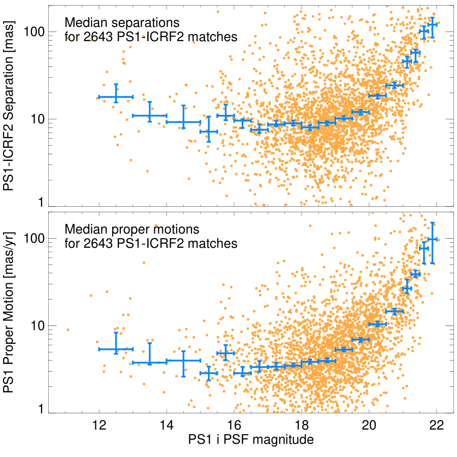
A cross-match with PS1 found 2679 objects within 0.5 arcsec of the ICRF2 positions.33 3 Unmatched objects are mainly below the declination limit, with a few falling into small holes in the PS1 sky coverage. Of those, 2643 are detected in the PS1 -band PSF magnitude. The positional and proper motion accuracies as function of magnitude are shown in Fig. 29. The scatter in this comparison is slightly larger than the PS1/Gaia cross-match (Figs. 9 and 10) because many ICRF2 optical counterparts are resolved galaxies or are blended with neighboring objects in the PS1 images. We have elected not to eliminate objects with ps-score less than 0.9 in this comparison because we wish to retain the fainter sources to get an estimate of the uncertainties below the Gaia magnitude limit.
Berghea et al. 2016 utilized a selected subset of ICRF2 sources to determine astrometric corrections for the PS1 catalog through the Global Astrometric Solution (GAS) method. The pre-release version of the PS1 catalog they used had an astrometric calibration based on 2MASS rather than on Gaia DR1 (which was not yet available). Their results removed the large scale errors in the PS1 DR1 due to its reference catalog. However, residual errors of about 60 mas remained in RA and declination that were correlated on small scales of a fraction of a degree. These small-scale errors are likely related to the errors that are corrected by our algorithm. Both the positions and proper motions from this paper are much more accurate than those from Berghea et al. 2016 because the higher sky density of the Gaia DR2 catalog enables the small-scale corrections that are required to remove distortions in the PS1 astrometry.
The comparison to ICRF2 also confirms the accuracy of our PS1 positions and proper motions to magnitudes fainter than the Gaia DR2 catalog detection limit. For objects in the magnitude range , the median error in the PS1 position is 8.7 mas, and the median error in the PM is 3.8 mas/yr. The errors increase for fainter objects, as expected due to noise in the PS1 images.
X Discussion and Summary
We have carried out a procedure to improve the astrometric accuracy of about 1.7 billion PS1 objects using Gaia DR2. In addition, we provide proper motions for these objects that are also corrected with Gaia. The astrometric correction procedure makes use of Gaia proper motions and parallaxes to shift the Gaia positions to the epochs of the PS1 objects. The PS1 DR2 catalog has systematic astrometric errors on a arcmin scale that are greatly reduced by our algorithm. For a subset of PS1 objects that are point-like (reference objects), the corrections result in mode (peak) and median PS1/Gaia positional residuals of about 4 mas and 9 mas, respectively, which is about a 33% reduction for the median (Fig. 3). The proper motions for these objects are corrected by a similar procedure to about 2 mas/yr (mode) and 5 mas/yr (median) compared with Gaia, which represents a 24% improvement for the median (see Fig. 4). The highest astrometric accuracy occurs for the most point-like objects and for intermediate magnitudes of about 17 mag (Figs. 7 to 10).
The positional corrections to a given PS1 object on the arcmin scale involves taking the median values of the PS1 to Gaia position shifts of the nearest 33 neighboring cross-matched objects, excluding the object itself (see Section III). In this process we are not force fitting positions of individual PS1 objects to cross-matched Gaia objects. Instead, we are smoothing spatial structures in the PS1/Gaia positional differences on the arcmin scale (Fig. 13). The correction process converges well with the number of nearest neighbors. For the 33 nearest neighbors that we apply, Figure 30 in Appendix A suggests that the results are converged to within about 1 mas. The corrections are applied to all PS1 objects that we consider, most of which do not cross match with a Gaia object. Similar corrections are applied to PS1 proper motions, although the improvements are not as large as for the positions.
The positional residuals in RA and declination are quite different (Fig. 14). The differences are minimized near zero zenith angle (see Fig. 15). The difference between the RA and declination residual distributions, as measured by the MAD of the residuals within stripes, varies with zenith angle and is proportional to the air mass (Fig. 18). The declination residuals within stripes vary with object color while the RA residuals are nearly independent of color (Fig. 19). The declination residual variations with color are much smaller in Stripe 16, which passes through the zenith, than at zenith angle 47 degrees (Stripes 2 and 30). These variations are consistent with the effects of atmospheric refraction that dispersively bend light rays by an amount that depends on declination. In principle, such color dependent effects could be calibrated and removed to provide a further reduction in residuals.
In the future, we intend to make these astrometry improvements available through MAST. There are also several areas for future improvements:
- 1.
While we have corrected the astrometry for 1.7 billion objects which have three or more detection epochs, over 8 billion other objects have two or fewer detection epochs. That includes many spurious detections, but also includes faint objects that are detected only on the stacked images that combine the single-epoch observations. We plan to apply our astrometric correction method to these objects as well.
- 2.
The systematic color-dependent residuals described in Section VII can be used to further improve the astrometric accuracy of the reference stars. The reference stars can in turn be used to make color-dependent corrections to the other PS1 objects. The inclusion of color-dependent corrections in our algorithm could result in substantial additional improvements in the astrometry, since the color terms appear large enough to account for much of the remaining scatter in the astrometric “sweet spot” around magnitude 17 (see Figs. 19 and 20).
- 3.
Our proper motion and parallax determinations are limited to smaller shifts over the range of PS1 epochs. The PS1 catalog splits measurements of detections that move more than 1 arcsec into separate objects, and the 2 arcsec PS1/Gaia cross matching that we initially apply also limits proper motions to less than about 0.7 mas/yr. Given the measured PMs of objects, it is likely that we can identify some that have multiple entries in the catalog and can re-unite them into single, more accurately measured objects.
We plan to reapply our corrections to PS1 astrometry as improved versions of the Gaia and PS1 catalogs become available. Our pipeline is well enough automated to make this possible without a lot of effort.
Acknowledgments
We thank Mike Fall and the Astrometry Working Group at STScI for motivating this work and providing feedback during the preliminary phase. In particular, we thank Stefano Casertano for examining the level of improvement that could be possible for PS1 astrometry by using Gaia. We also thank Ciprian Berghia, Valeri Makarov, and Juliene Frouard for insightful discussions about the limitations on the use of Gaia in the current PS1 astrometry. The Pan-STARRS1 Surveys (PS1) and the PS1 public science archive have been made possible through contributions by the Institute for Astronomy, the University of Hawaii, the Pan-STARRS Project Office, the Max-Planck Society and its participating institutes, the Max Planck Institute for Astronomy, Heidelberg and the Max Planck Institute for Extraterrestrial Physics, Garching, The Johns Hopkins University, Durham University, the University of Edinburgh, the Queen’s University Belfast, the Harvard-Smithsonian Center for Astrophysics, the Las Cumbres Observatory Global Telescope Network Incorporated, the National Central University of Taiwan, the Space Telescope Science Institute, the National Aeronautics and Space Administration under Grant No. NNX08AR22G issued through the Planetary Science Division of the NASA Science Mission Directorate, the National Science Foundation Grant No. AST-1238877, the University of Maryland, Eotvos Lorand University (ELTE), the Los Alamos National Laboratory, and the Gordon and Betty Moore Foundation.
References
- Berghea et al. (2016) Berghea, C. T., Makarov, V. V., Frouard, J., et al. 2016, AJ, 152, 53, doi: 10.3847/0004-6256/152/3/53
- Budavári & Lubow (2012) Budavári, T., & Lubow, S. H. 2012, ApJ, 761, 188, doi: 10.1088/0004-637X/761/2/188
- Budavári et al. (2010) Budavári, T., Szalay, A. S., & Fekete, G. 2010, PASP, 122, 1375, doi: 10.1086/657302
- Chambers et al. (2016) Chambers, K. C., Magnier, E. A., Metcalfe, N., et al. 2016, arXiv e-prints, arXiv:1612.05560. https://arxiv.org/abs/1612.05560
- Cudworth & Rees (1990) Cudworth, K. M., & Rees, R. 1990, AJ, 99, 1491, doi: 10.1086/115434
- Flewelling et al. (2016) Flewelling, H. A., Magnier, E. A., Chambers, K. C., et al. 2016, arXiv e-prints, arXiv:1612.05243. https://arxiv.org/abs/1612.05243
- Heasley (2008) Heasley, J. N. 2008, in American Institute of Physics Conference Series, Vol. 1082, American Institute of Physics Conference Series, ed. C. A. L. Bailer-Jones, 352–358, doi: 10.1063/1.3059075
- Lindegren et al. (2016) Lindegren, L., Lammers, U., Bastian, U., et al. 2016, A&A, 595, A4, doi: 10.1051/0004-6361/201628714
- Lindegren et al. (2018) Lindegren, L., Hernández, J., Bombrun, A., et al. 2018, A&A, 616, A2, doi: 10.1051/0004-6361/201832727
- Ma et al. (2009) Ma, C., Arias, E. F., Bianco, G., et al. 2009, IERS Technical Note, 35, 1
- Magnier et al. (2016) Magnier, E. A., Schlafly, E. F., Finkbeiner, D. P., et al. 2016, arXiv e-prints, arXiv:1612.05242. https://arxiv.org/abs/1612.05242
- Makarov et al. (2017) Makarov, V., Berghea, C. T., & Frouard, J. 2017, AADD USNO
- Schubert & Walterscheid (2000) Schubert, G., & Walterscheid, R. L. 2000, Earth, ed. A. N. Cox, 239
- Skrutskie et al. (2006) Skrutskie, M. F., Cutri, R. M., Stiening, R., et al. 2006, AJ, 131, 1163, doi: 10.1086/498708
- Tachibana & Miller (2018) Tachibana, Y., & Miller, A. A. 2018, PASP, 130, 128001, doi: 10.1088/1538-3873/aae3d9
- Thakar et al. (2003) Thakar, A. R., Szalay, A. S., Vandenberg, J. V., Gray, J., & Stoughton, A. S. 2003, Astronomical Society of the Pacific Conference Series, Vol. 295, Data Organization in the SDSS Data Release 1, ed. H. E. Payne, R. I. Jedrzejewski, & R. N. Hook, 217
- Tonry et al. (2012) Tonry, J. L., Stubbs, C. W., Lykke, K. R., et al. 2012, ApJ, 750, 99, doi: 10.1088/0004-637X/750/2/99
- Wallace (2018) Wallace, J. J. 2018, Research Notes of the American Astronomical Society, 2, 213, doi: 10.3847/2515-5172/aaf1a2
- Whitmore et al. (2016) Whitmore, B. C., Allam, S. S., Budavári, T., et al. 2016, AJ, 151, 134, doi: 10.3847/0004-6256/151/6/134
Appendix A Convergence of Position Shifts
We check that the corrected results are accurately determined using 33 nearest neighbors. To do this, we compare the corrected shifts in Stripe 2 () determined by 33 nearest neighbors with shifts resulting from using 16 and 50 nearest neighbors. For each corrected PS1 object, we compute the difference in shifts RA16 - RA33 that is the difference in the RA shift determinations using 16 and 33 neighbors. Similar calculations are done for the case of 50 nearest neighbors and for the declination. The distributions of these shift differences are plotted in Figure 30.
As expected, the distributions are narrower for the cases involving 50 neighbors than for 16 neighbors. The median absolute deviations (MAD) of the RA distributions are 1.6 mas and 0.9 mas for RA16 - RA33 and RA50 - RA33, respectively. The MADs of the Dec distributions are 1.8 mas and 1.0 mas for Dec16 - Dec33 and Dec50 - Dec33, respectively. These differences are much smaller than the typical position shifts, as seen in Figure 31. The MADs of RA50 - RA33 and Dec50 - Dec33, about 1 mas, give a measure of the uncertainty of shifts using the 33 nearest neighbors.
Appendix B Declination Ranges of Stripes
PS1 data is partitioned into 32 stripes based on source declination. Table 1 lists in columns the stripe number, the minimum declination, the maximum declination, and the average declination of the sources for each stripe. The declination values are in degrees.
| Stripe | Min | Max | Avg |
|---|---|---|---|
| ∘ | ∘ | ∘ | |
| 1 | -36.58 | -28.25 | -32.42 |
| 2 | -28.25 | -24.99 | -26.62 |
| 3 | -25.00 | -21.67 | -23.33 |
| 4 | -21.67 | -18.33 | -20.00 |
| 5 | -18.33 | -15.08 | -16.71 |
| 6 | -15.08 | -11.75 | -13.42 |
| 7 | -11.75 | -8.50 | -10.12 |
| 8 | -8.50 | -5.17 | -6.83 |
| 9 | -5.17 | -1.83 | -3.50 |
| 10 | -1.84 | 1.42 | -0.21 |
| 11 | 1.42 | 4.75 | 3.08 |
| 12 | 4.75 | 8.08 | 6.42 |
| 13 | 8.08 | 11.34 | 9.71 |
| 14 | 11.33 | 14.67 | 13.00 |
| 15 | 14.66 | 17.92 | 16.29 |
| 16 | 17.92 | 21.25 | 19.58 |
| 17 | 21.23 | 24.58 | 22.91 |
| 18 | 24.58 | 27.84 | 26.21 |
| 19 | 27.83 | 31.17 | 29.50 |
| 20 | 31.16 | 34.42 | 32.79 |
| 21 | 34.42 | 37.75 | 36.08 |
| 22 | 37.75 | 41.09 | 39.42 |
| 23 | 41.08 | 44.33 | 42.71 |
| 24 | 44.33 | 47.67 | 46.00 |
| 25 | 47.67 | 51.00 | 49.33 |
| 26 | 51.00 | 54.25 | 52.63 |
| 27 | 54.25 | 57.58 | 55.92 |
| 28 | 57.58 | 60.83 | 59.21 |
| 29 | 60.83 | 64.33 | 62.58 |
| 30 | 64.33 | 69.25 | 66.79 |
| 31 | 69.25 | 77.42 | 73.33 |
| 32 | 77.41 | 89.99 | 83.70 |