On Computational Poisson Geometry II:
Numerical Methods

M. Evangelista-Alvarado J. C. Ruíz-Pantaleón and P. Suárez-Serrato Address: Instituto de Matemáticas, Universidad Nacional Autónoma de México (UNAM), Mexico City, Mexico

doi:10.3934/jcd.2021012 J. Comput. Dyn. 8, 273–307 (2021)

Abstract

We present twelve numerical methods for evaluation of objects and concepts from Poisson geometry. We describe how each method works with examples, and explain how it is executed in code. These include methods that evaluate Hamiltonian and modular vector fields, compute the image under the coboundary and trace operators, the Lie bracket of differential 1–forms, gauge transformations, and normal forms of Lie–Poisson structures on $\mathbf{R}^{3}$ . The complexity of each of our methods is calculated, and we include experimental verifications on examples in dimensions two and three.

1 Introduction

This is our second paper in a series on the computational aspects of Poisson geometry. In the first paper we showed how fundamental concepts from Poisson geometry could be operationalized into symbolic code [19]. We also provided an associated Python module with our implementations, for ease of execution¹¹ 1 Available via https://github.com/appliedgeometry/poissongeometry.

A Poisson manifold [46, 56, 17, 32, 37] is a smooth manifold $M$ equipped with a contravariant skew–symmetric 2–tensor field $\Pi$ , called Poisson bivector field, satisfying the equation

[\hskip-1.84949pt[\Pi,\Pi]\hskip-1.84949pt]=0,

(1.1)

with respect to the Schouten–Nijenhuis bracket $[\hskip-1.84949pt[,]\hskip-1.84949pt]$ for multivector fields [43, 17]. Let $m=\dim{M}$ , and $x=(U;x^{1},\ldots,x^{m})$ be local coordinates on $M$ , then $\Pi$ has the following representation [39, 54]:

\Pi=\tfrac{1}{2}\Pi^{ij}\frac{\partial}{\partial{x^{i}}}\wedge\frac{\partial}{\partial{x^{j}}}\ =\sum_{1\leq i<j\leq m}\Pi^{ij}\frac{\partial}{\partial{x^{i}}}\wedge\frac{\partial}{\partial{x^{j}}}

(1.2)

The functions $\Pi^{ij}=\Pi^{ij}(x)\in\mathbf{\mathit{C}}^{\infty}_{U}$ are called the coefficients of $\Pi$ , and $\{\partial/\partial{x^{i}}\}$ is the canonical basis for vector fields on $U\subseteq M$ .

Poisson manifolds are generalizations of symplectic manifolds. A Poisson manifold can be thought of informally as a space that is foliated by symplectic leaves. It is then possible to define Hamiltonian dynamics relative to the symplectic forms defined on each leaf, via the Poisson bracket. Comprehensive treatments are available for interested readers [17, 37].

This geometric context provides a route that describes Hamiltonian dynamics rigorously. Applications of Hamiltonian dynamics are almost ubiquitous in every scientific domain. More specifically, uses of symplectic forms provide a formalism for diverse phenomena. This theory was introduced by Poisson himself to describe celestial mechanics [46]. It was then used by Dirac to investigate quantum mechanics [15], and notably Kontsevich showed that Poisson manifolds admit deformation quantizations [31].

In this paper, we present twelve methods that allow for numerical computations of concepts from Poisson geometry. These are listed in the following Table 1.1, along with their respective algorithms, and a list of (not exhaustive) relevant references for each one. We have indicated with an asterisk (*) the six methods that depend explicitly on our module for symbolic computation PoissonGeometry [19].

Table 1.1: Our numerical methods, with their corresponding algorithms, and examples where they are used. The right column is an informal summary of the algorithmic complexities, computed and presented in detail in Section 3.

Method	Algorithm	Examples	Complexity
num_bivector_field	1	[17, 8, 32, 37]	O( $m^{2}$ )
num_bivector_to_matrix	2	[17, 8, 32, 37]	O( $m^{2}$ )
num_hamiltonian_vf	3	[34, 8, 51, 7, 27]	O( $m^{2}$ )
num_poisson_bracket	4	[35, 17, 32, 37]	O( $m^{2}$ )
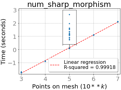
num_sharp_morphism	5	[17, 32, 37]	O( $m^{2}$ )
num_coboundary_operator *	6	[44, 17, 32, 3, 42]	O( $2^{m}$ )
num_modular_vf *	7	[2, 17, 32, 28, 37, 4, 45]	O( $2^{m}$ )
num_curl_operator *	8	[25, 14, 17, 37]	O( $2^{m}$ )
num_one_forms_bracket *	9	[17, 32, 37, 26]	O( $m^{2}$ )
num_gauge_transformation	10	[9, 5, 13]	O( $m^{7}$ )
num_linear_normal_form_R3 *	11	[40, 44, 24, 17, 49, 8, 37, 13, 42, 21]	O( $m$ )
num_flaschka_ratiu_bivector *	12	[25, 14, 23, 50, 18]	O( $m^{6}$ )

The following diagram illustrates the internal functional dependencies of the methods available in NumPoissonGeometry ²² 2 Avalaible via https://github.com/appliedgeometry/NumericalPoissonGeometry.

The methods presented here have classical applications to Mechanics—see for example [8]—and also to recent advances in computer-aided techniques for determining normal forms for Hamiltonian systems [10]. Furthermore, there has been a recent surge of interest in understanding Hamiltonian dynamics as uses of this theory start to appear in the data analysis and machine learning communities. Without attempting to be exhaustive, recent domains of application include; the development of Hamiltonian Monte Carlo techniques [16], applications of symplectic integration to optimization [41], inference of symbolic models from data [12], and the development of Hamiltonian Neural Networks [27, 53].

Our work has been specifically designed to be compatible with popular machine learning frameworks, as our code can be integrated into NumPy, Pytorch, or TensorFlow environments. Moreover, as we rely on lattice meshes for our evaluations, our results will also be of interest to researchers that use finite element methods.

We hope to contribute an additional dimension to the understanding of Poisson geometry, enabling everyone to carry out numerical experiments with our freely available open-source code, motivating the expansion of techniques that have so far been incorporated. To the best of our knowledge this is the first comprehensive implementation of these methods.

Our numerical techniques can inform and complement researchers’ intuition and provide further insights. For example, if a certain vector field is not trivial it can imply that a given Poisson structure is not unimodular, and this can be verified numerically. Moreover, our module only needs the algebraic expression for the Poisson bivector to carry out this verification (and not the complete, explicit vector field).

We have included specific examples for each of the methods above where numerical computations would be desirable, or are relevant in published work. We also strongly believe that our algorithms in this paper can be useful in the following related fields.

Our methods could aid in the development of deep learning systems for flows on tori and spheres [29], in particular for the groups $U(1)\cong\mathbf{S}^{1}$ and $SU(2)\cong\mathbf{S}^{3}$ . In a related direction, normalized flows on Lie groups have been investigated with respect to distributions of data points [20].

We expect our methods to be useful for evaluating inference problems related to the $n$ –body problem, which has been approached recently [6].

Hamiltonian dynamics have been used to learn systems of simulations [47]. This innovative work pioneers deep learning techniques that combine Hamiltonian dynamics and integrators of Ordinary Differential Equations. With our methods, such an overarching program could be extended to include more diverse equations, such as the ones that define a Poisson structure, or that verify conservation of specific quantities, for instance, a unimodular flow.

Normalized flows and techniques from symplectic geometry have been used to find canonical Darboux coordinates [38]. This highlights that the use of symplectic, and more generally, Poisson techniques is computationally efficient because these structures preserve volume.

Models that learn to respect conservative laws, through the use of Hamiltonian dynamics have been recently developed [27]. These could also be extended to more ample classes using our methods.

Hamiltonian functions themselves, relative to a symplectic form, have been modelled using recurrent neural networks [11]. We expect extensions of these works to be possible using our methods as well, where now the functions may be Hamiltonian relative to a Poisson structure. Moreover, systems that learn the dynamics from observed orbit trajectory data could be potentially designed.

There are two more applications that are relevant to the computation of statistical quantities on Lie groups. First, Hamiltonian flows that are equivariant with respect to an action can be used to learn densities that are invariant under the action of a Lie algebra. This strategy has been realized already for very specific algebras [30], and could be extended to more with our methods. Second, these ideas could also lead to a general method for finding reparametrizable densities on arbitrary Lie groups, using their associated Lie-Poisson structure [52].

This paper is organized in the following way. In section 2, we describe our algorithms and point to domains of application for each one. In section 3, detailed analyses of the complexities of our methods are presented, as well as experimental run-times. A summary with explicit upper bounds is found in Table 3.1.

2 Numerical Methods

—In this section we describe the implementation of all functions in NumPoissonGeometry and present numerical examples with classical/relevant Poisson bivector fields. Throughout this paper we will assume that the input functions used in our methods are computable.

2.1 NumPoissonGeometry: Evaluation

Our methods work with regular and irregular meshes that must be entered as NumPy arrays: a $(k,m)$ NumPy array for a mesh with $k$ points in $\mathbf{R}^{m}$ , for $k\in\mathbb{N}$ .

Irregular meshes can be used to implement probabilistic/statistical methods in Poisson geometry. In several of the subsections below we generate irregular meshes by means of random samples drawn from a uniform distribution over the interval $[0,1)$ . Sometimes for simplicity we use the ‘corners’ of the unit cube in $\mathbf{R}^{m}$ ,

Q^{m}:=\underset{m\text{\ times}}{\underbrace{\{0,1\}\ \times\cdots\times\{0,1\}}},

(2.1)

preloaded in Python into a NumPy array called Qmesh.

2.2 NumPoissonGeometry: Syntax

The instance and syntax of NumPoissonGeometry are the same as that of PoissonGeometry. We recall these here for the reader’s convenience.

Coordinates. By default, to emulate canonical coordinates on $\mathbf{R}^{m}$ , we use symbolic variables that are just the juxtaposition of the symbol x and an index of the set $\{1,\ldots,m\}$ : (x1, …, xm).

Scalar Functions. A scalar function is written using string literal expressions. For example, the function $f=ax_{1}^{2}+bx_{2}^{2}+cx_{3}^{2}$ should be written exactly as follows: ‘a*x1**2 + b*x2**2 + c*x3**2’. All characters that are not coordinates are treated as (symbolic) parameters: a, b and c for the previous example.

Multivector Fields and Differential forms. Both multivector fields and differential forms are written using dictionaries with tuples of integers as keys and string type values. If the coordinate expression of an $a$ –multivector field $A$ , with $a\in\mathbb{N}$ , is given by

A=\sum_{1\leq i_{1}<i_{2}<\cdots<i_{a}\leq m}A^{i_{1}i_{2}\cdots i_{a}}\frac{\partial}{\partial{x_{i_{1}}}}\wedge\frac{\partial}{\partial{x_{i_{2}}}}\wedge\cdots\wedge\frac{\partial}{\partial{x_{i_{a}}}},\quad A^{i_{1}\cdots i_{a}}=A^{i_{1}\cdots i_{a}}(x),

then $A$ should be written using a dictionary, as follows:

\Big\{(1,...,a):\mathscr{A}^{1\cdots a},\,...,\,(i_{1},...,i_{a}):\mathscr{A}^{i_{1}\cdots i_{a}},\,...,\,(m-a+1,...,m):\mathscr{A}^{m-a+1\cdots m}\Big\}

(2.2)

Here, each key $(i_{1},\ldots,i_{a})$ is a tuple containing ordered indices $1\leq i_{1}<\cdots<i_{a}\leq m$ and the corresponding value $\mathscr{A}^{i_{1}\cdots i_{a}}$ is the string expression of the scalar function (coefficient) $A^{i_{1}\cdots i_{a}}$ of $A$ .

The syntax for differential forms is the same. It is important to remark that we can only write the keys and values of non–zero coefficients. See the documentation for more details.

2.3 NumPoissonGeometry: Python Implementation

First let us briefly describe the syntax of the module NumPoissonGeometry. The inputs of the twelve methods in Table 1.1 have to be string literal expressions (or dictionaries containing them). The sympify method converts such string expressions into symbolic variables, and the lambdify method transforms the symbolic expressions into functions that allow a (fast) numerical evaluation.

The output of our methods can be chosen to be a NumPy array (by default) or a pytorch/tensorflow tensor containing the evaluation of the input data at each point in a mesh on $\mathbf{R}^{m}$ .

Next we will explain each of our numerical methods, how they relate to the theoretical objects being implemented, present the corresponding algorithm, and show how they may be used with helpful examples.

2.4 Bivector Fields

The evaluation of a (Poisson) bivector field $\Pi$ at a point in $M$ is defined by

\Pi_{p}:=\tfrac{1}{2}\Pi^{ij}(p)\left.\frac{\partial}{\partial{x^{i}}}\right|_{p}\wedge\left.\frac{\partial}{\partial{x^{j}}}\right|_{p},\quad p\in M.

Observe that the coefficients of $\Pi$ in (1.2) at $p$ determines the evaluation above.

The function num_bivector evaluates a (Poisson) bivector field on a mesh in $\mathbf{R}^{m}$ .

Algorithm 1 num_bivector(bivector, mesh)

Input:

a (Poisson) bivector field and a mesh

Output:

evaluation of the bivector field at each point of the mesh

1: procedure

m

\leftarrow

dimension of the manifold

3: bivector

\leftarrow

a variable encoding the (Poisson) bivector field

4: mesh

\leftarrow

(k,m)

array encoding the mesh

\triangleright

k

: number of points in the mesh

5: Transform each bivector item into a function that allows a numerical evaluation

6: return an array containing the evaluation of bivector at each

m

–array of mesh

7: end procedure

Example 2.1.

Consider the Lie–Poisson bivector field on $\mathbf{R}^{3}_{x}$

\Pi_{\mathfrak{so}(3)}=x_{3}\frac{\partial}{\partial x_{1}}\wedge\frac{\partial}{\partial x_{2}}-x_{2}\frac{\partial}{\partial x_{1}}\wedge\frac{\partial}{\partial x_{3}}+x_{1}\frac{\partial}{\partial x_{2}}\wedge\frac{\partial}{\partial x_{3}},

(2.3)

associated to the 3–dimensional Lie algebra $\mathfrak{so}(3)$ , which is used in studies of the 3–body problem [7], and more generally in geometric mechanics [8]. To evaluate $\Pi_{\mathfrak{so}(3)}$ at points of $Q^{3}$ in (2.1) we compute:

Note that the output preserves the PoissonGeometry syntax (2.2). For example, to produce a PyTorch tensor encoding this information we use the pt_output flag:

Refer to caption — Figure 2.1: *Left*: Symplectic foliation of $\Pi_{\mathfrak{so}(3)}$ in (2.3). *Right*: Modular vector field of $\Pi$ in (2.13) relative to the Euclidean volume form on $\mathbf{R}^{3}$ . The color scale indicates the magnitude of the vectors.

2.5 Matrix of a Bivector Field

The value of the matrix (field) $[\Pi^{ij}]$ of $\Pi$ at a point $p\in M$ is defined to be the matrix

\big[\Pi^{ij}\big]_{p}:=\big[\Pi^{ij}(p)\big].

(2.4)

Hence, we just need to know the value of the coefficients of $\Pi$ in (1.2) at $p$ .

The function num_bivector_to_matrix evaluates the matrix of a (Poisson) bivector field on a mesh in $\mathbf{R}^{m}$ .

Algorithm 2 num_bivector_to_matrix(bivector, mesh)

Input:

a (Poisson) bivector field and a mesh

Output:

evaluation of the matrix of the (Poisson) bivector field at each point of the mesh

1: procedure

m

\leftarrow

dimension of the manifold

3: bivector

\leftarrow

a variable encoding the (Poisson) bivector field

4: mesh

\leftarrow

(k,m)

array encoding the mesh

\triangleright

k

: number of points in the mesh

5: variable_1

\leftarrow

a variable encoding the matrix of the (Poisson) bivector field

6: Transform each variable_1 item into a function that allows a numerical evaluation

7: return an array containing the evaluation of variable_1 at each

m

–array of mesh

8: end procedure

Example 2.2.

Consider the Lie–Poisson bivector field on $\mathbf{R}^{3}_{x}$

\Pi_{\mathfrak{sl}(2)}=-x_{3}\frac{\partial}{\partial x_{1}}\wedge\frac{\partial}{\partial x_{2}}-x_{2}\frac{\partial}{\partial x_{1}}\wedge\frac{\partial}{\partial x_{3}}+x_{1}\frac{\partial}{\partial x_{2}}\wedge\frac{\partial}{\partial x_{3}},

(2.5)

associated to the 3–dimensional Lie algebra $\mathfrak{sl}(2)$ , used in the classification of rigid motions [13], and in other mechanical systems [44, 8]. To evaluate the matrix of $\Pi_{\mathfrak{sl}(2)}$ at points of $Q^{3}$ in (2.1) we compute:

2.6 Hamiltonian Vector Fields

The Hamiltonian vector field $X_{h}:=\mathbf{i}_{\mathrm{d}{h}}\Pi$ of a scalar function $h$ , and relative to a Poisson bivector field $\Pi$ on $M$ , at a point in $M$ can be determined by the following (coordinate) formula:

X_{h}|_{p}=-\left[\Pi^{ij}(p)\right]\left[\tfrac{\partial h}{\ \partial x^{k}}(p)\right],\quad p\in M

(2.6)

Here, $[\Pi^{ij}]$ is the matrix of $\Pi$ in (2.4) and $[{\partial h}/{\partial x^{k}}]$ is the gradient vector (field) of $h$ , for $k=1,\ldots,m$ .

The function num_hamiltonian_vf evaluates a Hamiltonian vector field on a mesh in $\mathbf{R}^{m}$ .

Algorithm 3 num_hamiltonian_vf(bivector, ham_function, mesh)

Input:

a Poisson bivector field $\Pi$ , a scalar function $h$ and a mesh

Output:

evaluation of the Hamiltonian vector field of $h$ respect to $\Pi$ at each point of the mesh

1: procedure

m

\leftarrow

dimension of the manifold

3: bivector

\leftarrow

a variable encoding the Poisson bivector field

\Pi

4: ham_function

\leftarrow

an expression representing the scalar function

h

5: mesh

\leftarrow

(k,m)

array encoding the mesh

\triangleright

k

: number of points in the mesh

6: variable_1

\leftarrow

the (symbolic) gradient vector field of ham_function

7: Transform each variable_1 item into a function that allows a numerical evaluation

8: variable_2

\leftarrow

an array containing the evaluation of variable_1 at each

m

–array of mesh

9: variable_3

\leftarrow

num_bivector_to_matrix( bivector, mesh)

\triangleright

see Algorithm 2

10: variable_4

\leftarrow

an empty container

11: for

0\leq i<k

12: variable_4[

i

]

\leftarrow

(-1)

*

variable_3[

i

]

*

variable_2[

i

]

\triangleright

matrix–vector product

13: end for

14: return variable_4

15: end procedure

Example 2.3.

Consider the Hamiltonian vector field on $\mathbf{R}^{6}_{x}$ , that arises in a particular case of the three body problem [7],

X_{h}=-x_{4}\frac{\partial}{\partial{x_{1}}}-x_{5}\frac{\partial}{\partial{x_{2}}}-x_{6}\frac{\partial}{\partial{x_{3}}}+\left[\tfrac{1}{(x_{1}-x_{2})|x_{1}-x_{2}|}+\tfrac{1}{(x_{1}-x_{3})|x_{1}-x_{3}|}\right]\frac{\partial}{\partial{x_{4}}}\\ +\left[\tfrac{1}{(x_{1}-x_{2})|x_{1}-x_{2}|}+\tfrac{1}{(x_{2}-x_{3})|x_{2}-x_{3}|}\right]\frac{\partial}{\partial{x_{5}}}-\left[\tfrac{1}{(x_{1}-x_{3})|x_{1}-x_{3}|}+\tfrac{1}{(x_{2}-x_{3})|x_{2}-x_{3}|}\right]\frac{\partial}{\partial{x_{6}}},

with Hamiltonian function

h=\frac{1}{x_{1}-x_{2}}+\frac{1}{x_{1}-x_{3}}+\frac{1}{x_{2}-x_{3}}+\frac{x_{4}^{2}+x_{5}^{2}+x_{6}^{2}}{2},

(2.7)

and relative to the canonical Poisson bivector field on $\mathbf{R}^{6}_{x}$

\Pi=\frac{\partial}{\partial x_{1}}\wedge\frac{\partial}{\partial x_{4}}+\frac{\partial}{\partial x_{2}}\wedge\frac{\partial}{\partial x_{5}}+\frac{\partial}{\partial x_{3}}\wedge\frac{\partial}{\partial x_{6}}.

(2.8)

To evaluate $X_{h}$ avoiding singularities we use the mesh, for $Q^{3}$ being as in (2.1),

\{-2,-1\}\times\{0,1\}\times\{2,3\}\times Q^{3},\quad\mathbf{R}^{6}=\mathbf{R}^{3}_{\scriptscriptstyle(x_{1},x_{2},x_{3})}\times\mathbf{R}^{3}_{\scriptscriptstyle(x_{4},x_{5},x_{6})}:

2.7 Poisson Brackets

The Poisson bracket $\{f,g\}_{\Pi}$ of two scalar functions $f$ and $g$ , induced by a Poisson bivector field $\Pi$ on $M$ , at a point in $M$ can be calculated in coordinates following formulas in [17, Section 1.2]:

\{f,g\}_{\Pi}(p)=-\big[\tfrac{\partial g}{\partial x^{k}}(p)\big]^{\top}\left[\Pi^{ij}(p)\right]\big[\tfrac{\partial f}{\partial x^{l}}(p)\big],\quad p\in M

Here, $[\Pi^{ij}]$ is the matrix of $\Pi$ in (2.4), $[{\partial f}/{\partial x^{l}}]$ and $[{\partial g}/{\partial x^{k}}]$ are the gradient vector (fields) of $f$ and $g$ , in that order, for $k,l=1,\ldots,m$ .

The function num_poisson_bracket evaluates the Poisson bracket of two scalar functions on a mesh in $\mathbf{R}^{m}$ .

Algorithm 4 num_poisson_bracket(bivector, function_1, function_2, mesh)

Input:

a Poisson bivector field $\Pi$ , two scalar functions $f,g$ and a mesh

Output:

evaluation of the Poisson bracket of $f$ and $g$ induced by $\Pi$ at each point of the mesh

1: procedure

m

\leftarrow

dimension of the manifold

3: bivector

\leftarrow

a variable encoding the Poisson bivector field

\Pi

4: function_1, function_2

\leftarrow

expressions representing the functions

f

and

g

5: mesh

\leftarrow

(k,m)

array encoding the mesh

\triangleright

k

: number of points in the mesh

6: if function_1

-

function_2

==0

then

7: return 0

\triangleright

f=g

, then its Poisson bracket is zero

8: else

9: variable_1

\leftarrow

the (symbolic) gradient vector field of function_2

10: Transform each variable_1 item into a function that allows a numerical evaluation

11: variable_2

\leftarrow

an array containing the evaluation of variable_1 at each

m

–array of mesh

12: variable_3

\leftarrow

num_hamiltonian_vf( bivector, function_1, mesh)

13:

\triangleright

see Algorithm 3

14: variable_4

\leftarrow

an empty container

15: for

0\leq i<k

16: variable_4[

i

]

\leftarrow

variable_2[

i

]

*

variable_3[

i

]

\triangleright

scalar vector product

17: end for

18: return variable_4

19: end if

20: end procedure

Example 2.4.

Consider the Poisson bivector field on $\mathbf{R}^{6}_{x}$ , obtained as a deformation of an almost Poisson structure analyzed in relation to plasma [36] (see, also [48]),

\Pi=\frac{\partial}{\partial x_{1}}\wedge\frac{\partial}{\partial x_{4}}+\frac{\partial}{\partial x_{2}}\wedge\frac{\partial}{\partial x_{5}}+\frac{\partial}{\partial x_{3}}\wedge\frac{\partial}{\partial x_{6}}+x_{2}^{2}\frac{\partial}{\partial x_{5}}\wedge\frac{\partial}{\partial x_{6}}.

(2.9)

Observe that the Poisson bracket $\{x_{6},x_{5}\}_{\Pi}=-1$ , at points $x\in\mathbf{R}^{6}$ such that $|x_{2}|=1$ . We can check this fact using random meshes of the form

\{a_{1},b_{1}\}\times\{1\}\times\{a_{2},b_{2}\}\times\cdots\times\{a_{5},b_{5}\},\qquad a_{i},b_{i}\in\operatorname{random}{[0,1)}.

Here, random samples are taken from a uniform distribution over the interval $[0,1)$ :

Observe that we use a probabilistic method to verify a particular property of a Poisson bracket. These methods can be used to determine other characteristics, for example, singular points.

2.8 Sharp Morphism

In the context of Lie algebroids, the vector bundle morphism $\Pi^{\sharp}:\alpha\mapsto\mathbf{i}_{\alpha}\Pi$ , induced by a Poisson bivector field $\Pi$ on $M$ , is the anchor map of the Poisson Lie algebroid corresponding to $\Pi$ [22].

Similarly to (2.6), we can evaluate the image $\Pi^{\sharp}(\alpha)$ of a differential 1–form $\alpha$ at a point in $M$ as follows:

\Pi^{\sharp}(\alpha)\big|_{p}=-\left[\Pi^{ij}(p)\right]\big[\alpha_{k}(p)\big],\quad p\in M

(2.10)

Here, $[\Pi^{ij}]$ is the matrix of $\Pi$ in (2.4) and $[\alpha_{k}]$ is the coefficient vector of $\alpha=\alpha_{k}\mathrm{d}{x^{k}}$ , for $k=1,\ldots,m$ .

The function num_sharp_morphism evaluates a vector field $\Pi^{\sharp}(\alpha)$ on a mesh in $\mathbf{R}^{m}$ .

Algorithm 5 num_sharp_morphism(bivector, one_form, mesh)

Input:

a Poisson bivector field $\Pi$ , a differential 1–form $\alpha$ and a mesh

Output:

evaluation of the vector field $\Pi^{\sharp}(\alpha)$ at each point of the mesh

1: procedure

m

\leftarrow

dimension of the manifold

3: bivector

\leftarrow

a variable encoding the Poisson bivector field

\Pi

4: one_form

\leftarrow

a variable encoding the differential 1–form

\alpha=\alpha_{1}\mathrm{d}{x^{1}}+\cdots+\alpha_{m}\mathrm{d}{x^{m}}

5: mesh

\leftarrow

(k,m)

array encoding the mesh

\triangleright

k

: number of points in the mesh

6: variable_1

\leftarrow

a container with items

(\alpha_{1},\ldots,\alpha_{m})

7: Transform each variable_1 item into a function that allows a numerical evaluation

8: variable_2

\leftarrow

an array containing the evaluation of variable_1 at each

m

–array of mesh

9: variable_3

\leftarrow

num_bivector_to_matrix( bivector, mesh)

\triangleright

see Algorithm 2

10: variable_4

\leftarrow

an empty container

11: for

0\leq i<k

12: variable_4[

i

]

\leftarrow

(-1)

*

variable_3[

i

]

*

variable_2[

i

]

\triangleright

matrix–vector product

13: end for

14: return variable_4

15: end procedure

Example 2.5.

Consider the Casimir function $K=({1}/{2})(x_{1}^{2}+x_{2}^{2}+x_{3}^{2})$ of the Poisson bivector field $\Pi_{\mathfrak{so}(3)}$ in (2.3) [14, 7]. By definition, the exterior derivative of $K$ ,

\mathrm{d}{K}=x_{1}\mathrm{d}{x_{1}}+x_{2}\mathrm{d}{x_{2}}+x_{3}\mathrm{d}{x_{3}},

(2.11)

belongs to the kernel of $\Pi_{\mathfrak{so}(3)}$ , that is, $\Pi_{\mathfrak{so}(3)}^{\sharp}(\mathrm{d}{K})=0$ . We can check this fact by using random meshes:

2.9 Coboundary Operator

The coboundary operator $\delta_{\Pi}:\Gamma\wedge^{\bullet}T{M}\rightarrow\Gamma\wedge^{\bullet+1}T{M}$ induced by a Poisson bivector field $\Pi$ on $M$ [39] is defined by

\delta_{\Pi}(A):=[\hskip-1.84949pt[\Pi,A]\hskip-1.84949pt],\quad A\in\Gamma\wedge T{M}.

Here, $\Gamma\wedge^{\bullet}T{M}$ denotes the module of multivector fields on $M$ .

The function num_coboundary_operator evaluates the image under $\delta_{\Pi}$ of an arbitrary multivector field on a mesh in $\mathbf{R}^{m}$ .

Algorithm 6 num_coboundary_operator(bivector, multivector, mesh)

Input:

a Poisson bivector field $\Pi$ , a multivector field $A$ and a mesh

Output:

evaluation of the multivector field $[\hskip-1.84949pt[\Pi,A]\hskip-1.84949pt]$ at each point of the mesh

1: procedure

m

\leftarrow

dimension of the manifold

3: bivector

\leftarrow

a variable encoding the Poisson bivector field

\Pi

4: multivector

\leftarrow

a variable encoding the multivector field

A

5: mesh

\leftarrow

(k,m)

array encoding the mesh

\triangleright

k

: number of points in the mesh

6: variable_1

\leftarrow

a variable encoding the image of multivector under the coboundary operator induced by bivector

\triangleright

We use the lichnerowicz_poisson_operator method of PoissonGeometry

8: Transform each variable_1 item into a function that allows a numerical evaluation

9: return an array containing the evaluation of variable_1 at each

m

–array of mesh

10: end procedure

Example 2.6.

The vector field on $\mathbf{R}^{3}_{x}\setminus\{x_{3}\text{--axis}\}$

W=\frac{x_{1}x_{3}e^{{-1}/{(x_{1}^{2}+x_{2}^{2}-x_{3}^{2})^{2}}}}{x_{1}^{2}+x_{2}^{2}}\frac{\partial}{\partial{x_{1}}}+\frac{x_{2}x_{3}e^{{-1}/{(x_{1}^{2}+x_{2}^{2}-x_{3}^{2})^{2}}}}{x_{1}^{2}+x_{2}^{2}}\frac{\partial}{\partial{x_{2}}}\\ +e^{{-1}/{(x_{1}^{2}+x_{2}^{2}-x_{3}^{2})^{2}}}\frac{\partial}{\partial{x_{3}}}

(2.12)

arises in the study of the first cohomology group of the Poisson bivector field $\Pi_{\mathfrak{sl}(2)}$ in (2.5) to construct a 1–cocycle that is not Hamiltonian [44, 42]. To check the cocycle property of $W$ under the coboundary operator induced by $\Pi_{\mathfrak{sl}(2)}$ , we evaluate the (image) bivector field $[\hskip-1.84949pt[\Pi_{\mathfrak{sl}(2)},W]\hskip-1.84949pt]$ on random meshes:

The characteristic foliation of $\Pi_{\mathfrak{sl}(2)}$ can be described using the Casimir function $2K=x_{1}^{2}+x_{2}^{2}-x_{3}^{2}$ (see, Figure 2.2). Observe that $W$ is orthogonal to the gradient vector field of $K$ , $x_{1}\partial/\partial{x_{1}}+x_{2}\partial/\partial{x_{2}}-x_{3}\partial/\partial{x_{3}}$ . Hence, $W$ is tangent to the symplectic foliation of $\Pi_{\mathfrak{sl}(2)}$ (see, Figure 2.2). However, $W$ can be extended to a smooth vector field on all of $\mathbf{R}^{3}$ that is not Hamiltonian with respect to $\Pi_{\mathfrak{sl}(2)}$ [44]. Therefore the first Poisson cohomology group of $\Pi_{\mathfrak{sl}(2)}$ is non–trivial.

2.10 Modular Vector Field

The modular vector field of an orientable Poisson manifold $(M,\Pi)$ is an infinitesimal automorphism of $\Pi$ determined by the choice of a volume form $\Omega$ [55], and it is defined by the linear map

Z_{\Pi,\Omega}:h\longmapsto\mathrm{div}_{\Omega}X_{h},\quad h\in\mathbf{\mathit{C}}^{\infty}_{M}.

Here, $\mathrm{div}_{\Omega}X_{h}\in\mathbf{\mathit{C}}^{\infty}_{M}$ denotes the divergence of the Hamiltonian vector field $X_{h}$ (2.6) with respect to $\Omega$ .

The modular vector field measures how far Hamiltonian flows are from preserving a given volume form [55]. In the regular case, the existence of a volume form that remains invariant under every Hamiltonian vector field only depends on the characteristic (symplectic) foliation of the Poisson manifold, rather than the leaf–wise symplectic form [2]. In particular, for regular codimension–one symplectic foliations, a characteristic class controls the existence of such a volume form [28].

The function num_modular_vf evaluates the modular vector field of a Poisson bivector field on a mesh in $\mathbf{R}^{m}$ .

Algorithm 7 num_modular_vf(bivector, function, mesh)

Input:

a Poisson bivector field $\Pi$ , a non–zero scalar function $f_{0}$ and a mesh

Output:

evaluation of the modular vector field of $\Pi$ relative to the volume form $f_{0}\Omega_{0}$ at each point of the mesh. Where $\Omega_{0}$ is the Euclidean volume form on $\mathbf{R}^{m}$

1: procedure

m

\leftarrow

dimension of the manifold

3: bivector

\leftarrow

a variable encoding the Poisson bivector field

\Pi

4: function

\leftarrow

an expression representing the scalar function

f_{0}

5: mesh

\leftarrow

(k,m)

array encoding the mesh

\triangleright

k

: number of points in the mesh

6: variable_1

\leftarrow

a variable encoding the modular vector field of bivector with respect to the volume form ( function)

\cdot\Omega_{0}

\triangleright

We use the modular_vf method of PoissonGeometry

7: Transform each variable_1 item into a function that allows a numerical evaluation

8: return an array containing the evaluation of variable_1 at each

m

–array of mesh

9: end procedure

Example 2.7.

The characteristic foliation of the following homogeneous Poisson bivector field on $\mathbf{R}^{3}_{x}$ coincides with that of $\Pi_{\mathfrak{so}(3)}$ in (2.3):

\Pi=\tfrac{1}{4}x_{3}\big(x_{1}^{4}+x_{2}^{4}+x_{3}^{4}\big)\frac{\partial}{\partial x_{1}}\wedge\frac{\partial}{\partial x_{2}}-\tfrac{1}{4}x_{2}\big(x_{1}^{4}+x_{2}^{4}+x_{3}^{4}\big)\frac{\partial}{\partial x_{1}}\wedge\frac{\partial}{\partial x_{3}}\\ +\tfrac{1}{4}x_{1}\big(x_{1}^{4}+x_{2}^{4}+x_{3}^{4}\big)\frac{\partial}{\partial x_{2}}\wedge\frac{\partial}{\partial x_{3}}

(2.13)

However, $(\mathbf{R}^{3},\Pi_{\mathfrak{so}(3)})$ admits a Hamiltonian–invariant volume form, while $\Pi$ does not [45]. Consequently, the following vector field,

Z_{\Pi}=\big(x_{2}x_{3}^{3}-x_{2}^{3}x_{3}\big)\frac{\partial}{\partial{x_{1}}}+\big(x_{3}x_{1}^{3}-x_{3}^{3}x_{1}\big)\frac{\partial}{\partial{x_{2}}}+\big(x_{1}x_{2}^{3}-x_{1}^{3}x_{2}\big)\frac{\partial}{\partial{x_{3}}},

which is the modular vector field of $\Pi$ with respect to the Euclidean volume form on $\mathbf{R}^{3}_{x}$ , cannot be a Hamiltonian vector field.

We can now use random meshes to check numerically that there are points for which the modular vector field of $\Pi$ with respect to the Euclidean volume form is not zero, which implies that $\Pi$ is not unimodular, as follows:

Observe that $Z_{\Pi}$ is orthogonal to the radial vector field $x_{i}\partial/\partial{x_{i}}$ on $\mathbf{R}^{3}_{x}$ , for $i=1,2,3$ . As the characteristic foliation of $\Pi$ consists of the origin and concentric spheres (see, Figure 2.1), $Z_{\Pi}$ is tangent to the symplectic leafs of $\Pi$ .

2.11 Curl Operator

On an oriented manifold $M$ with volume form $\Omega$ , the divergence of an $a$ –multivector field $A$ on $M$ [33], and relative to $\Omega$ , is the unique $(a-1)$ –multivector field $\mathscr{D}_{\Omega}(A)$ on $M$ such that

\mathbf{i}_{\mathscr{D}_{\Omega}(A)}\Omega=\mathrm{d}{\mathbf{i}_{A}}\Omega.

(2.14)

The function num_curl_operator evaluates the divergence of a multivector field on a mesh in $\mathbf{R}^{m}$ . Let $\Omega_{0}$ denote the standard volume form on $\mathbf{R}^{m}$ :

Algorithm 8 num_curl_operator(multivector, function, mesh)

Input:

a multivector field $A$ , a non–zero scalar function $f_{0}$ and a mesh

Output:

evaluation of the the divergence of $A$ with respect to the volume form $f_{0}\Omega_{0}$ at each point of the mesh.

1: procedure

m

\leftarrow

dimension of the manifold

3: multivector

\leftarrow

a variable encoding the multivector field

A

4: function

\leftarrow

an expression representing the scalar function

f_{0}

5: mesh

\leftarrow

(k,m)

array encoding the mesh

\triangleright

k

: number of points in the mesh

6: variable_1

\leftarrow

a variable encoding the divergence of bivector with respect to the volume form ( function)

\cdot\Omega_{0}

\triangleright

We use the curl_operator method of PoissonGeometry

7: Transform each variable_1 item into a function that allows a numerical evaluation

8: return an array containing the evaluation of variable_1 at each

m

–array of mesh

9: end procedure

Example 2.8.

The next Poisson bivector field on $\mathbf{R}^{4}_{x}$ , has been applied to the analyze the orbital stability of the Pais–Uhlenbeck oscillator [4],

\Pi=2x_{4}\frac{\partial}{\partial x_{1}}\wedge\frac{\partial}{\partial x_{3}}+2x_{3}\frac{\partial}{\partial x_{1}}\wedge\frac{\partial}{\partial x_{4}}-2x_{4}\frac{\partial}{\partial x_{2}}\wedge\frac{\partial}{\partial x_{3}}+2x_{3}\frac{\partial}{\partial x_{2}}\wedge\frac{\partial}{\partial x_{4}}\\ +(x_{1}-x_{2})\frac{\partial}{\partial x_{3}}\wedge\frac{\partial}{\partial x_{4}}.

(2.15)

It is unimodular on (the whole of) $\mathbf{R}^{4}_{x}$ , and has trivial modular vector field with respect to the Euclidean volume form. For a fixed volume form, the divergence of a Poisson bivector field coincides with its (minus) modular vector field. Hence, the unimodularity of $\Pi$ in (2.15) may be numerically verified, at least in a sample, using random meshes. In this example the output is a Pytorch tensor:

2.12 Differential 1–Forms Bracket

In the context of Lie algebroids, the Koszul bracket of 1–forms is the Lie bracket on the space of sections of a Poisson Lie algebroid [33, 26].

By definition and (2.10), the Lie bracket of two differential 1–forms $\alpha$ and $\beta$ , induced by a Poisson bivector field $\Pi$ on $M$ , at a point in $M$ can be determined by the following (coordinate) formula:

\{\alpha,\beta\}_{\Pi}(p)=\big[(\mathrm{d}{\beta})_{kl}(p)\big]\left[\Pi^{ij}(p)\right]\big[\alpha_{r}(p)\big]-\big[(\mathrm{d}{\alpha})_{kl}(p)\big]\left[\Pi^{ij}(p)\right]\big[\beta_{r}(p)\big]\\ -\big[\tfrac{\partial}{\partial x^{r}}\big(\left[\beta_{k}\right]^{\top}\left[\Pi^{ij}\right]\left[\alpha_{l}\right]\big)(p)\big],\quad p\in M

Here, $[\Pi^{ij}]$ is the matrix of $\Pi$ in (2.4), $[(\mathrm{d}{\alpha})_{kl}]$ and $[(\mathrm{d}{\beta})_{kl}]$ are the matrix of the differential 2–forms $\mathrm{d}{\alpha}=1/2\,(\mathrm{d}{\alpha})_{kl}\mathrm{d}{x^{k}}\wedge\mathrm{d}{x^{l}}$ and $\mathrm{d}{\beta}=1/2\,(\mathrm{d}{\beta})_{kl}\mathrm{d}{x^{k}}\wedge\mathrm{d}{x^{l}}$ , $[\alpha_{r}]$ and $[\beta_{r}]$ are the coefficient vectors of $\alpha=\alpha_{k}\mathrm{d}{x^{k}}$ and $\beta=\beta_{k}\mathrm{d}{x^{k}}$ , and $[{\partial}/{\partial x^{r}}(\cdot)]$ is the gradient vector (field) operator, for $k,l,r=1,\ldots,m$ .

The function num_one_forms_bracket evaluates the differential 1–form $\{\alpha,\beta\}_{\Pi}$ on a mesh in $\mathbf{R}^{m}$ .

Algorithm 9 num_one_forms_bracket(bivector, one_form_1, one_form_2, mesh)

Input:

a Poisson bivector field $\Pi$ , two differential 1–forms $\alpha,\beta$ and a mesh

Output:

evaluation of the Lie bracket of $\alpha$ and $\beta$ induced by $\Pi$ at each point of the mesh

1: procedure

m

\leftarrow

dimension of the manifold

3: bivector

\leftarrow

a variable encoding the Poisson bivector field

\Pi

4: one_form_1

\leftarrow

a variable encoding the differential 1–form

\alpha=\alpha_{1}\mathrm{d}{x^{1}}+\cdots+\alpha_{m}\mathrm{d}{x^{m}}

5: one_form_2

\leftarrow

a variable encoding the differential 1–form

\beta=\beta_{1}\mathrm{d}{x^{1}}+\cdots+\beta_{m}\mathrm{d}{x^{m}}

6: mesh

\leftarrow

(k,m)

array encoding the mesh

\triangleright

k

: number of points in the mesh

7: variable_1

\leftarrow

a container with items

(\alpha_{1},\ldots,\alpha_{m})

8: variable_2

\leftarrow

a container with items

(\beta_{1},\ldots,\beta_{m})

9: for

i\in\{1,2\}

10: variable_3_

i

\leftarrow

the (symbolic) Jacobian matrix of variable_

i

11:

\triangleright

variable_

i

thought of as a vector field

12: Transform each variable_3_i item into a function that allows a numerical evaluation

13: variable_4_

i

\leftarrow

an array containing the evaluation of variable_3_

i

at each

m

–array of mesh

14: variable_5_

j

\leftarrow

num_sharp_morphism( bivector, one_form_

j

, mesh)

15:

\triangleright

i\neq j=1,2

. See Algorithm 2

16: end for

17: variable_6, variable_7

\leftarrow

empty containers

18: for

0\leq i<k

19: variable_6[

i

]

\leftarrow

( variable_4_1

-

transpose( variable_4_1))[

i

]

*

variable_5_2[

i

]

20: variable_7[

i

]

\leftarrow

( variable_4_2

-

transpose( variable_4_2))[

i

]

*

variable_5_1[

i

]

21:

\triangleright

matrix–vector products

22: end for

23: variable_8

\leftarrow

a variable encoding the image of one_form_

j

under the sharp morphism induced by bivector

\triangleright

We use the sharp_morphism method of PoissonGeometry

24: variable_9

\leftarrow

variable_8

*

variable_2

\triangleright

scalar vector product

25: variable_10

\leftarrow

the (symbolic) gradient vector field of variable_9

26: Transform each variable_10 item into a function that allows a numerical evaluation

27: variable_11

\leftarrow

an array containing the evaluation of variable_10 at each

m

–array of mesh

28: variable_12

\leftarrow

an empty container

29: for

0\leq i<k

30: variable_12[

i

]

\leftarrow

variable_7[

i

]

-

variable_6[

i

]

+

variable_11[

i

]

\triangleright

vector sum

31: end for

32: return variable_12

33: end procedure

Example 2.9.

By definition, the Lie bracket induced by the Poisson bivector field $\Pi$ in (2.9) [36], see also [48], of the (basic) differential 1–forms $\mathrm{d}{x_{5}}$ and $\mathrm{d}{x_{6}}$ is given by

\{\mathrm{d}{x_{5}},\mathrm{d}{x_{6}}\}_{\Pi}=2x_{2}\mathrm{d}{x_{2}}.

Hence, $\{\mathrm{d}{x_{5}},\mathrm{d}{x_{6}}\}_{\Pi}=2\mathrm{d}{x_{2}}$ at points $x\in\mathbf{R}^{6}$ such that $x_{2}=1$ . This coincides with the following computation involving random meshes,

\{a_{1},b_{1}\}\times\{1\}\times\{a_{2},b_{2}\}\times\cdots\times\{a_{5},b_{5}\},\quad a_{i},b_{i}\in\operatorname{random}{[0,1]}:

2.13 Gauge Transformations

Gauge transformations are used to simplify dynamical equations, they aid in reduction methods for dynamical systems. They are also used for the hamiltonization of nonholonomic systems [5]. Recall that the hamiltonization problem consists in determining conditions that represent a dynamical system in Hamiltonian form.

Given a differential 2–form $\lambda$ on $M$ , if the morphism $\mathrm{id}_{T^{\ast}{M}}-\lambda^{\flat}\circ\Pi^{\sharp}$ is invertible, the $\lambda$ –gauge transformation of a bivector field $\Pi$ on $M$ is the bivector field $\overline{\Pi}$ determined by the vector bundle morphism ${\overline{\Pi}}^{\sharp}=\Pi^{\sharp}\circ(\mathrm{id}_{T^{\ast}{M}}-\lambda^{\flat}\circ\Pi^{\sharp})^{-1}$ [48]. This morphism can be evaluated at a point in $M$ as follows:

\overline{\Pi}^{\sharp}_{p}=-\big[\Pi^{ij}(p)\big]\left(\mathrm{I}-\big[\lambda_{kl}(p)\big]\big[\Pi^{ij}(p)\big]\right)^{-1},\quad p\in M

Here, $[\Pi^{ij}]$ is the matrix of $\Pi$ in (2.4), $[\lambda_{kl}]$ is the matrix of $\lambda=1/2\,\lambda_{kl}\mathrm{d}{x^{k}}\wedge\mathrm{d}{x^{l}}$ and $\mathrm{I}$ denotes the $m\times m$ identity matrix, for $k,l=1,\ldots,m$ . The morphism $\lambda^{\flat}:T{M}\rightarrow T^{\ast}{M}$ above is given by $X\mapsto\mathbf{i}_{X}\lambda$ .

The function num_gauge_transformation evaluates the gauge transformation of a bivector field on a mesh in $\mathbf{R}^{m}$ .

Algorithm 10 num_gauge_transformation(bivector, two_form, mesh)

Input:

a (Poisson) bivector field $\Pi$ , a differential 2–form $\lambda$ and a mesh

Output:

evaluation of the gauge transformation of $\Pi$ induced by $\lambda$ at each point of the mesh

1: procedure

m

\leftarrow

dimension of the manifold

3: bivector

\leftarrow

a variable encoding the (Poisson) bivector field

\Pi

4: two_form

\leftarrow

a variable encoding the (Poisson) the differential 2–form

\lambda

5: mesh

\leftarrow

(k,m)

array encoding the mesh

\triangleright

k

: number of points in the mesh

6: variable_1

\leftarrow

num_bivector_to_matrix( bivector, mesh)

\triangleright

see Algorithm 2

7: variable_2

\leftarrow

num_bivector_to_matrix( two_form, mesh)

\triangleright

see Algorithm 2

8: variable_3

\leftarrow

the identity

m\times m

matrix

9: variable_4

\leftarrow

an empty container

10: for

0\leq i<k

11: variable_4[

i

]

\leftarrow

variable_3

-

variable_2[

i

]

*

variable_1[

i

]

12:

\triangleright

matrix sum/multiplication

13: end for

14: variable_5

\leftarrow

an empty container

15: for

0\leq i<k

16: if determinant( variable_4[

i

])

\neq 0

then

17: variable_5[

i

]

\leftarrow

variable_1[

i

]

*

inverse( variable_4[

i

])

\triangleright

matrix multiplication

18: else

19: variable_5[

i

]

\leftarrow

False

20: end if

21: end for

22: return variable_5

23: end procedure

Example 2.10.

For this example we will use the following result that we proved in [19]:

Proposition 1.

Let $\Pi$ be a bivector field on a 3–dimensional smooth manifold $M$ . Then, given a differential 2–form $\lambda$ on $M$ , the $\lambda$ –gauge transformation $\overline{\Pi}$ of $\Pi$ is well defined on the open subset,

\big\{F:=1+\big\langle\lambda,\Pi\big\rangle\neq 0\big\}\subseteq M.

(2.16)

Moreover, $\overline{\Pi}$ is given by

\overline{\Pi}=\tfrac{1}{F}\Pi.

In consequence, if $\Pi$ is Poisson, then $\overline{\Pi}$ is also Poisson.

Observe that if $\langle\lambda,\Pi\rangle=0$ in (2.16), then $\Pi$ remains unchanged under the gauge transformation induced by $\lambda$ . This holds for the Poisson bivector field $\Pi_{\mathfrak{so}(3)}$ in (2.3) [7] and the differential 2–form on $\mathbf{R}^{3}$ given by

\lambda=(x_{1}-x_{2})\mathrm{d}{x_{1}}\wedge\mathrm{d}{x_{2}}+(x_{1}-x_{3})\mathrm{d}{x_{1}}\wedge\mathrm{d}{x_{3}}+(x_{2}-x_{3})\mathrm{d}{x_{2}}\wedge\mathrm{d}{x_{3}}.

(2.17)

Then, for $Q^{3}$ being as in (2.1), we can check the invariance of $\Pi_{\mathfrak{so}(3)}$ under $\lambda$ as follows:

Notice that the output is the same as the second one in Example 2.1, which encodes the evaluation of the bivector field $\Pi_{\mathfrak{so}(3)}$ at points of $Q^{3}$ .

2.14 Lie–Poisson Normal Forms on $\mathbf{R}^{3}$

Two Poisson bivector fields $\Pi$ and $\widetilde{\Pi}$ on $M$ are said to be equivalent (or isomorphic) if there exists a diffeomorphism $F:M\rightarrow M$ such that $\widetilde{\Pi}=F^{\ast}\Pi$ . Under this equivalence relation there exist 9 non–trivial normal forms of Lie–Poisson bivector fields on $\mathbf{R}^{3}$ [40, 49].

The function num_linear_normal_form_R3 evaluates a normal form of a given Lie–Poisson bivector field on a mesh in $\mathbf{R}^{3}$ .

Algorithm 11 num_linear_normal_form_R3(linear_bivector, mesh)

Input:

a Lie–Poisson bivector field $\Pi$ on $\mathbf{R}^{3}$ and a mesh

Output:

evaluation of a normal form of $\Pi$ at each point of the mesh

1: procedure

m

\leftarrow

dimension of the manifold

3: linear_bivector

\leftarrow

a variable that encodes the Lie–Poisson bivector field

\Pi

4: mesh

\leftarrow

(k,m)

array encoding the mesh

\triangleright

k

: number of points in the mesh

5: variable_1

\leftarrow

a variable encoding a linear normal form of linear_bivector

\triangleright

We use the linear_normal_form_R3 method of PoissonGeometry

7: return num_bivector( variable_1, mesh)

\triangleright

see Algorithm 1

8: end procedure

Example 2.11.

Using the function linear_normal_form_R3 of PoissonGeometry we can verify that the Lie–Poisson bivector field on $\mathbf{R}^{3}_{x}$

\Pi=2(x_{2}+x_{3})\frac{\partial}{\partial x_{1}}\wedge\frac{\partial}{\partial x_{2}}+(x_{1}-x_{2})\frac{\partial}{\partial x_{1}}\wedge\frac{\partial}{\partial x_{3}}+(x_{1}+x_{2}+2x_{3})\frac{\partial}{\partial x_{2}}\wedge\frac{\partial}{\partial x_{3}},

(2.18)

admits the following Poisson bivector field as a normal form:

\Pi_{N}=(x_{1}-4ax_{2})\frac{\partial}{\partial x_{1}}\wedge\frac{\partial}{\partial x_{3}}+(4ax_{1}+x_{2})\frac{\partial}{\partial x_{2}}\wedge\frac{\partial}{\partial x_{3}},\quad a>0

To evaluate this normal form of $\Pi$ at points of $Q^{3}$ (2.1) we compute:

The equivalence between $\Pi$ and $\Pi_{N}$ implies that the characteristic foliation of $\Pi$ is a open book foliation [21], as shown in Figure 2.3 below. In particular, $\Pi$ does not admit global, non–constant, Casimir functions.

2.15 Flaschka–Ratiu Poisson Bivector Field

If $M$ is a oriented manifold with volume form $\Omega$ , the Poisson bivector field $\Pi$ determined by $m-2$ prescribed Casimir functions $K_{1},...,K_{m-2}$ on $M$ , and defined by the formula

\mathbf{i}_{\Pi}\Omega=\mathrm{d}{K_{1}}\wedge\cdots\wedge\mathrm{d}{K_{m-2}},

is called Flaschka–Ratiu bivector field [25, 14]. Observe that $\Pi$ is non–trivial on the open subset of $M$ where $K_{1},\ldots,K_{m-2}$ are (functionally) independent.

The function num_flaschka_ratiu_bivector evaluates a Flaschka–Ratiu bivector field on a mesh in $\mathbf{R}^{m}$ .

Algorithm 12 num_flaschka_ratiu_bivector(casimirs_list, mesh)

Input:

a set of scalar functions and a mesh

Output:

evaluation of the Flaschka–Ratiu bivector field induced by these functions at each point of the mesh

1: procedure

m

\leftarrow

dimension of the manifold

3: casimirs_list

\leftarrow

a container with

m-2

(string) expressions representing the set of scalar functions

\triangleright

each string expression represents a scalar function

4: mesh

\leftarrow

(k,m)

array encoding the mesh

\triangleright

k

: number of points in the mesh

5: variable_1

\leftarrow

a variable encoding the Flaschka–Ratiu bivector field induced by casimirs_list

\triangleright

We use the flaschka_ratiu_bivector method of PoissonGeometry

6: return num_bivector( variable_1, mesh)

\triangleright

see Algorithm 1

7: end procedure

Example 2.12.

Consider the following (Poisson) Flaschka–Ratiu bivector field on $\mathbf{R}^{4}_{x}$

\Pi=x_{3}\frac{\partial}{\partial x_{1}}\wedge\frac{\partial}{\partial x_{2}}-x_{2}\frac{\partial}{\partial x_{1}}\wedge\frac{\partial}{\partial x_{3}}-x_{1}\frac{\partial}{\partial x_{2}}\wedge\frac{\partial}{\partial x_{3}},

that appears as a local model around singularities of a broken Lefschetz fibration on smooth 4–manifolds [23] (see, also [50, 18]). It is induced by the functions

K_{1}=\tfrac{1}{2}x_{4},\quad K_{2}=-x_{1}^{2}+x_{2}^{2}+x_{3}^{2}.

(2.19)

To evaluate $\Pi$ at points of $Q^{4}$ (2.1) we compute:

3 Algorithmic Complexity and Performance

In this section we will present an approximation to the (worst–case) time complexity of the twelve algorithms in Table 1.1, as well as a time performance analysis of our Python implementation of the functions in the module NumPoissonGeometry. Recall that we are assuming the input functions to be computable.

3.1 Complexity

The time complexity of certain algorithms depends on the nature and structure of the input data. In our methods two important processes in the implementation depend on the length of the input data items: converting string expressions to symbolic variables, and transforming these symbolic expressions into functions that allow a numerical evaluation. Therefore, for the analysis of our algorithms we define,

|C|:=\underset{x\,\in\,C}{\operatorname{max}}\,\{\mathrm{len}(x)\},

for a container $C$ with (string expression) items that encode the coefficients (scalar functions) of the coordinate expression of a multivector field or a differential form. For example, as illustrated in (2.2), we use dictionaries for our Python implementation. In this case, $C$ is a tuple (or list) that contains all the values of a such dictionary.

In the following Table 3.1 we record the approximate worst–case time complexities for the twelve methods of our NumPoissonGeometry module:

Table 3.1: Worst–case time complexity of NumPoissonGeometry methods. In the second column:

m

denotes the dimension of

\mathbf{R}^{m}

k

is the number of points in a mesh on

\mathbf{R}^{m}

, we denote by

[\cdot]

the integer part function and by

\mathrm{comb}

a combination.

Method	Time Complexity
01. num_bivector_field	$\mathscr{O}(m^{2}k\|bivector\|)$
02. num_bivector_to_matrix	$\mathscr{O}(m^{2}k\|bivector\|)$
03. num_hamiltonian_vf	$\mathscr{O}(mk(m\|bivector\|+\mathrm{len}(ham\_function)))$
04. num_poisson_bracket	$\mathscr{O}(mk(m\|bivector\|+\mathrm{len}(function\_1)+\mathrm{len}(function\_2)))$
05. num_sharp_morphism	$\mathscr{O}(m(mk\|bivector\|+\|one\_form\|))$
06. num_coboundary_operator	$\mathscr{O}(\mathrm{comb}(m,[m/2])\|bivector\|\mathrm{len}(function)(m^{5}+k))$
07. num_modular_vf	$\mathscr{O}(\mathrm{comb}(m,[m/2])\|bivector\|\mathrm{len}(function)(m+k))$
08. num_curl_operator	$\mathscr{O}(\mathrm{comb}(m,[m/2])\|multivector\|\mathrm{len}(function)(m+k))$
09. num_one_forms_bracket	$\mathscr{O}(m^{2}k\|bivector\|\|one\_form\_1\|\|one\_form\_2\|)$
10. num_gauge_transformation	$\mathscr{O}\big(m^{2}k(m^{5}+\|bivector\|+\|two\_form\|)\big)$
11. num_linear_normal_form_R3	$\mathscr{O}(k\|bivector\|)$
12. num_flaschka_ratiu_bivector	$\mathscr{O}(m^{6}k\|bivector\|)$

Remark 3.1.

Observe that the time complexities in Table 3.1 depend linearly on the number of points in the mesh ( $k$ ).

Recall that the time complexity of independent processes equals the sum of the respective time complexities of each process. With this in mind, we present the deduction of the time complexities of our numerical methods presented in Table 3.1.

3.1.1 Polynomial Complexity

The following methods have polynomial time complexities.

Lemma 3.2.

The time complexity of the num_bivector_field method is approximately

\mathscr{O}(m^{2}k|bivector|).

Proof.

Consider the Algorithm 1 with bivector and mesh inputs. The time complexity of our implementation depends on:

i.

Line 5 $\rightarrow$ $\mathscr{O}(m^{2}|bivector|)$ : we iterate over bivector, and the transformation of each bivector item depends on its length.
ii.

Line 6 $\rightarrow$ $\mathscr{O}(km^{2}|bivector|)$ : we iterate over mesh, and the evaluation of bivector depends on its length and on the length of its items.

Hence, the time complexity of num_bivector_field is $\mathscr{O}(m^{2}k|bivector|)$ . ∎

Lemma 3.3.

The time complexity of the num_bivector_to_matrix method is approximately

\mathscr{O}(m^{2}k|bivector|).

Proof.

Consider the Algorithm 2 with bivector and mesh inputs. The time complexity of our implementation depends on:

i.

Line 5 $\rightarrow$ $\mathscr{O}(m^{2}|bivector|)$
ii.

Line 6 $\rightarrow$ $\mathscr{O}(m^{2}|bivector|)$ : we iterate over the $m\times m$ matrix variable_1, and the transformation of each bivector item depends on its length.
iii.

Line 7 $\rightarrow$ $\mathscr{O}(km^{2}|bivector|)$ : we iterate over mesh, and the evaluation of variable_1 depends on its dimension and on the length of the bivector items.

Hence, the time complexity of num_bivector_to_matrix is $\mathscr{O}(m^{2}k|bivector|)$ . ∎

Lemma 3.4.

The time complexity of the num_hamiltonian_vf method is approximately

\mathscr{O}(mk(m|bivector|+\mathrm{len}(ham\_function)))

Proof.

Consider the Algorithm 3 with bivector, ham_function and mesh inputs. The time complexity of our implementation depends on:

i.

Line 6 $\rightarrow$ $\mathscr{O}(m\mathrm{len}(ham\_function))$ : calculate the gradient of ham_function depends on the length of this expression and on the dimension of $\mathbf{R}^{m}$ .
ii.

Line 7 $\rightarrow$ $\mathscr{O}(m\mathrm{len}(ham\_function))$ : we iterate over the $m\times 1$ matrix variable_1, and the transformation of each of its items depends on the length of ham_function.
iii.

Line 8 $\rightarrow$ $\mathscr{O}(km\mathrm{len}(ham\_function))$ : we iterate over mesh, and the evaluation of variable_1 depends on its dimension and on the length of ham_function.
iv.

Line 9 $\rightarrow$ $\mathscr{O}(m^{2}k|bivector|)$ : the num_bivector_to_matrix method has time complexity $\mathscr{O}(m^{2}k|bivector|)$ .
v.

Lines 11-13 $\rightarrow$ $\mathscr{O}(km^{2})$ : we iterate over the set of indices $\{0,\ldots,k-1\}$ , and the product of the variable_2 and variable_3 items has time complexity $\mathscr{O}(m^{2})$ .

Hence, the time complexity of num_hamiltonian_vf is

\mathscr{O}(mk(m|bivector|+\mathrm{len}(ham\_function))).

∎

Lemma 3.5.

The time complexity of the num_poisson_bracket method is approximately

\mathscr{O}(mk(m|bivector|+\mathrm{len}(function\_1)+\mathrm{len}(function\_2))).

Proof.

Consider the Algorithm 4 with bivector, function_1, function_2 and mesh inputs. The time complexity of our implementation depends on:

i.

Line 9 $\rightarrow$ $\mathscr{O}(m\mathrm{len}(function\_2))$ : calculate the gradient of function_2 depends on the length of this expression and on the dimension of $\mathbf{R}^{m}$ .
ii.

Line 10 $\rightarrow$ $\mathscr{O}(m\mathrm{len}(function\_2))$ : we iterate over the $m\times 1$ matrix variable_1, and the transformation of each of its items depends on the length of function_2.
iii.

Line 11 $\rightarrow$ $\mathscr{O}(km\mathrm{len}(function\_2))$ : we iterate over mesh, and the evaluation of variable_1 depends on its dimension and on the length of function_2.
iv.

Line 12 $\rightarrow$ $\mathscr{O}(mk(m|bivector|+\mathrm{len}(function\_1)))$ : the num_hamiltonian_vf has time complexity $\mathscr{O}(mk(m|bivector|+\mathrm{len}(ham\_function)))$ .
v.

Lines 14-16 $\rightarrow$ $\mathscr{O}(km^{2})$ : we iterate over the set of indices $\{0,\ldots,k-1\}$ , and the product of the variable_2 and variable_3 items has time complexity $\mathscr{O}(m^{2})$ .

Hence, the time complexity of num_poisson_bracket is

\mbox{$\mathscr{O}(mk(m|bivector|+\mathrm{len}(function\_1)+\mathrm{len}(function\_2)))$}.

∎

Lemma 3.6.

The time complexity of the num_sharp_morphism method is approximately

\mathscr{O}(m(mk|bivector|+|one\_form|)).

Proof.

Consider the Algorithm 5 with bivector, one_form and mesh inputs. The time complexity of our implementation depends on:

i.

Line 7 $\rightarrow$ $\mathscr{O}(m|one\_form|)$ : we iterate over the $(m,1)$ container variable_1, and the transformation of each of its items depends on the length of one_form items.
ii.

Line 9 $\rightarrow$ $\mathscr{O}(m^{2}k|bivector|)$ : the num_bivector_to_matrix method has time complexity $\mathscr{O}(m^{2}k|bivector|)$ .
iii.

Lines 11-13 $\rightarrow$ $\mathscr{O}(km^{2})$ : we iterate over the set of indices $\{0,\ldots,k-1\}$ , and the product of the variable_2 and variable_3 items has time complexity $\mathscr{O}(m^{2})$ .

Hence, the time complexity of num_sharp_morphism is

\mathscr{O}(m(mk|bivector|+|one\_form|)).

∎

Lemma 3.7.

The time complexity of the num_one_forms_bracket method is approximately

\mathscr{O}(m^{2}k|bivector|\\ |one\_form\_1||one\_form\_2|)

Proof.

Consider the Algorithm 9 with bivector, one_form_1, one_form_2 and mesh inputs. The time complexity of our implementation depends on:

i.

Line 10 $\rightarrow$ $\mathscr{O}(m^{2}(|one\_form\_1|+|one\_form\_2|))$ : calculate the Jacobian matrix of variable_i depends on the length of one_form_1 and one_form_2 items and on the dimension of $\mathbf{R}^{m}$ .
ii.

Line 11 $\rightarrow$ $\mathscr{O}(m^{2}(|one\_form\_1|+|one\_form\_2|))$ : we iterate over the $m\times m$ matrix variable_3_i, and the transformation of each of its items depends on the length of one_form_1 and one_form_2 items.
iii.

Line 13 $\rightarrow$ $\mathscr{O}(m(mk|bivector|+|one\_form\_1|+|one\_form\_2|))$ : the num_sharp_ morphism method has time complexity $\mathscr{O}(m(mk|bivector|+|one\_form|))$ .
iv.

Lines 16-19 $\rightarrow$ $\mathscr{O}(km^{2})$ : we iterate over the set of indices $\{0,\ldots,k-1\}$ , and the product of the variable_4_i and variable_5_j items has time complexity $\mathscr{O}(m^{2})$ , for $i,j=1,2$ .
v.

Line 20 $\rightarrow$ $\mathscr{O}(m^{2}|bivector||one\_form\_1|)$ : the sharp_morphism method has time complexity $\mathscr{O}(m^{2}|bivector||one\_form|)$ .
vi.

Line 22 $\rightarrow$ $\mathscr{O}(m|one\_form\_1||one\_form\_2|)$ : calculate the gradient of variable_9 depends on the length of one_form_1 and one_form_2 items, and on the dimension of $\mathbf{R}^{m}$ .
vii.

Line 23 $\rightarrow$ $\mathscr{O}(m(|one\_form\_1||one\_form\_2|))$ : we iterate over the $m\times 1$ matrix variable_10, and the transformation of each of its items depends on the length of one_form_1 and one_form_2 items.
viii.

Lines 26-28 $\rightarrow$ $\mathscr{O}(km)$ : we iterate over the set of indices $\{0,\ldots,k-1\}$ , and the sum of variables variable_6, variable_7 and variable_11 items has time complexity $\mathscr{O}(m)$ .

Hence, the time complexity of num_one_forms_bracket is

\mathscr{O}(m^{2}k|bivector||one\_form\_1||one\_form\_2|).

∎

Lemma 3.8.

The time complexity of the num_gauge_transformation method is approximately $\mathscr{O}(m^{2}k(m^{5}+|bivector|+|two\_form|))$ .

Proof.

Consider the Algorithm 10 with bivector, two_form and mesh inputs. The time complexity of our implementation depends on:

i.

Line 6 $\rightarrow$ $\mathscr{O}(m^{2}k|bivector|)$ : the num_bivector_to_matrix method has time complexity $\mathscr{O}(m^{2}k|bivector|)$ .
ii.

Line 7 $\rightarrow$ $\mathscr{O}(m^{2}k|two\_form|)$ : the num_bivector_to_matrix method has complexity
$\mathscr{O}(m^{2}k|bivector|)$ .
iii.

Lines 10-12 $\rightarrow$ $\mathscr{O}(km^{2})$ : we iterate over the set of indices $\{0,\ldots,k-1\}$ , and the matrix operations between the variable_1, variable_2 and variable_3 items has time complexity $\mathscr{O}(m^{2})$ .
iv.

Lines 14-20 $\rightarrow$ $\mathscr{O}(km^{10})$ : we iterate over the set of indices $\{0,\ldots,k-1\}$ , calculate the determinant of each item of variable_4 has time complexity $\mathscr{O}(m^{4})$ , the inverse has time complexity $\mathscr{O}(m^{3})$ , and the matrix product in line 16 has time complexity $\mathscr{O}(m^{3})$ .

Hence, the time complexity of num_gauge_transformation is

\mathscr{O}(m^{2}k(m^{5}+|bivector|+|two\_form|)).

∎

Lemma 3.9.

The time complexity of the num_linear_normal_form_R3 method is approximately $\mathscr{O}(k|bivector|)$ .

Proof.

Consider the Algorithm 11 with linear_bivector and mesh inputs. The time complexity of our implementation depends on:

i.

Line 5 $\rightarrow$ $\mathscr{O}(|bivector|)$ : the linear_normal_form_R3 method has time complexity $\mathscr{O}(|bivector|)$ .
ii.

Line 6 $\rightarrow$ $\mathscr{O}(k|bivector|)$ : the num_bivector_field method has time complexity $\mathscr{O}(m^{2}k|bivector|)$ .

Hence, the time complexity of num_linear_normal_form_R3 is $\mathscr{O}(k|bivector|)$ . ∎

Lemma 3.10.

The time complexity of the num_flaschka_ratiu_bivector method is approximately $\mathscr{O}(m^{6}k|bivector|)$ .

Proof.

Consider the Algorithm 12 with casimir_list and mesh inputs. The time complexity of our implementation depends on:

i.

Line 5 $\rightarrow$ $\mathscr{O}(m^{6}|casimir\_list|)$ : the flaschka_ratiu_bivector method has complexity
$\mathscr{O}(m^{6}|casimir\_list|)$ .
ii.

Line 6 $\rightarrow$ $\mathscr{O}(m^{2}k|casimir\_list|)$ : the num_bivector_field method has time complexity
$\mathscr{O}(m^{2}k|bivector|)$ .

Hence, the time complexity is $\mathscr{O}(m^{6}k|bivector|)$ . ∎

3.1.2 Exponential Complexity

Due to the nature of the concatenated loops in our methods, and because we need to calculate ordered index permutations, the following methods have exponential time complexities.

Lemma 3.11.

The time complexity of the num_coboundary_operator method is approximately $\mathscr{O}(\mathrm{comb}(m,[m/2])|bivector|\mathrm{len}(function)(m^{5}+k))$ .

Proof.

Consider the Algorithm 6 with bivector, multivector and mesh inputs. The time complexity of our implementation depends on:

i.

Line 6 $\rightarrow$ $\mathscr{O}(m^{5}\mathrm{comb}(m,[m/2])|bivector||multivector|)$ : the lichnerowicz_poisson_ operator method has time complexity

$\mathscr{O}(m^{5}\mathrm{comb}(m,[m/2])|bivector||multivector|).$
ii.

Line 7 $\rightarrow$ $\mathscr{O}(\mathrm{comb}(m,[m/2])|bivector||multivector|)$ : we iterate over variable_1, and the transformation of each of its items depends on the length of the bivector and multivector items.
iii.

Line 8 $\rightarrow$ $\mathscr{O}(k\mathrm{comb}(m,[m/2])|bivector||multivector|)$ : we iterate over mesh, and the evaluation of variable_1 depends on its length and on the length of the bivector and multivector items.

Hence, the time complexity of num_coboundary_operator is

\mbox{$\mathscr{O}(\mathrm{comb}(m,[m/2])|bivector|\mathrm{len}(function)(m^{5}+k))$}.

∎

Lemma 3.12.

The time complexity of the num_modular_vf method is approximately

\mathscr{O}(\mathrm{comb}(m,[m/2])|bivector|\mathrm{len}(function)(m+k)).

Proof.

Consider the Algorithm 7 with bivector, function and mesh inputs. The time complexity of our implementation depends on:

i.

Line 6 $\rightarrow$ $\mathscr{O}(m\,\mathrm{comb}(m,[m/2])|bivector|\mathrm{len}(function))$ : the modular_vf method has time complexity $\mathscr{O}(m\,\mathrm{comb}(m,[m/2])|bivector|\mathrm{len}(function))$ .
ii.

Line 7 $\rightarrow$ $\mathscr{O}(\mathrm{comb}(m,[m/2])|bivector|\mathrm{len}(function))$ : we iterate over variable_1, and the transformation of each of its items depends on the length of the bivector items and the function string expression.
iii.

Line 8 $\rightarrow$ $\mathscr{O}(k\mathrm{comb}(m,[m/2]|bivector|\mathrm{len}(function)))$ : we iterate over mesh. The evaluation of variable_1 depends on its length, and on the length of the bivector items and the function string expression.

Hence, the time complexity of num_modular_vf is

\mathscr{O}(\mathrm{comb}(m,[m/2])|bivector|\mathrm{len}(function)(m+k)).

∎

Lemma 3.13.

The time complexity of the num_curl_operator method is approximately

\mathscr{O}(\mathrm{comb}(m,[m/2])|multivector|\mathrm{len}(function)(m+k)).

Proof.

Consider the Algorithm 8 with bivector, function and mesh inputs. The time complexity of our implementation depends on:

i.

Line 6 $\rightarrow$ $\mathscr{O}(m\,\mathrm{comb}(m,[m/2])|multivector|\mathrm{len}(function))$ : the curl_operator method has time complexity $\mathscr{O}(m\,\mathrm{comb}(m,[m/2])|multivector|\mathrm{len}(function))$ .
ii.

Line 7 $\rightarrow$ $\mathscr{O}(\mathrm{comb}(m,[m/2])|multivector|\mathrm{len}(function))$ : we iterate over variable_1, and the transformation of each of its items depends on the length of the multivector items and the function string expression.
iii.

Line 8 $\rightarrow$ $\mathscr{O}(k\mathrm{comb}(m,[m/2]|multivector|\mathrm{len}(function)))$ : we iterate over mesh. The evaluation of variable_1 depends on its length, and on the length of the multivector items and the function string expression.

Hence, the time complexity of num_curl_operator is

\mbox{$\mathscr{O}(\mathrm{comb}(m,[m/2])|multivector|\mathrm{len}(function)(m+k))$}.

∎

3.2 Performance

The time performance of each function in NumPoissonGeometry was experimentally measured by evaluating concrete examples on $\mathbf{R}^{2}$ , and $\mathbf{R}^{3}$ , on precalculated (irregular) meshes with $10^{\kappa}$ points, for $\kappa=3,\ldots,7$ . These meshes were generated by means of random samples extracted from a uniform distribution in the interval $[0,1)$ .

All the numerical experiments were performed on a workstation equipped with 48 GB of main memory in a 3 $\times$ 16 GB ddr4 module configuration and an Intel(R) Core(TM) i7-6700 CPU @ 3.40GHz CPU, running at 3.4 GHz for a peak theoretical performance of four cores.

3.2.1 Two Dimensional Case

For the performance tests of our methods in dimension two, we have set the non–degenerate Poisson bivector field

\Pi_{0}=\frac{\partial}{\partial x_{1}}\wedge\frac{\partial}{\partial x_{2}},

induced by the standard symplectic structure $\mathrm{d}{x_{1}}\wedge\mathrm{d}{x_{2}}$ on $\mathbf{R}^{2}_{x}$ .

Table 3.2: Input data used for the time performance tests of functions 1-10 in Table 3.3.

Function	Input	Function	Input
1	$\Pi_{0}$	6	$\Pi_{0}$ , $W=x_{2}\frac{\partial}{\partial x_{1}}-x_{1}\frac{\partial}{\partial x_{2}}$
2	$\Pi_{0}$	7	$\Pi_{0}$ , $f=1$
3	$\Pi_{0}$ , $h=x_{1}^{2}+x_{2}^{2}$	8	$\Pi_{0}$ , $f=1$
4	$\Pi_{0}$ , $f=x_{1}^{2}+x_{2}^{2}$ , $g=x_{1}+x_{2}$	9	$\Pi_{0}$ , $\alpha=x_{1}\mathrm{d}{x_{1}}+x_{2}\mathrm{d}{x_{2}}$ , $\beta=\mathrm{d}{x_{1}}+\mathrm{d}{x_{2}}$
5	$\Pi_{0}$ , $\alpha=x_{1}\mathrm{d}{x_{1}}+x_{2}\mathrm{d}{x_{2}}$	10	$\Pi_{0}$ , $\lambda=\mathrm{d}{x_{1}}\wedge\mathrm{d}{x_{2}}$

Table 3.3 lists the mean time in seconds (with standard deviation) it takes to evaluate the first ten functions in NumPoissonGeometry (see, Table 1.1) on a irregular mesh on $\mathbf{R}^{3}_{x}$ with $10^{\kappa}$ points, computed by taking twenty-five samples, for $\kappa=3,\ldots,7$ .

Table 3.3: Summary of the time performance of NumPoissonGeometry functions, in dimension two.

Function	Points in mesh/Processing time (in seconds)
Function	$10^{3}$	$10^{4}$	$10^{5}$	$10^{6}$	$10^{7}$
01. num_bivector_field	0.004 $\pm$ 0.689	0.038 $\pm$ 0.009	0.356 $\pm$ 0.002	3.545 $\pm$ 0.026	35.711 $\pm$ 0.164
02. num_bivector_to_matrix	0.006 $\pm$ 3.633	0.046 $\pm$ 0.001	0.438 $\pm$ 0.004	4.442 $\pm$ 0.037	45.155 $\pm$ 1.466
03. num_hamiltonian_vf	0.014 $\pm$ 0.001	0.112 $\pm$ 0.006	1.096 $\pm$ 0.021	10.867 $\pm$ 0.044	108.460 $\pm$ 0.726
04. num_poisson_bracket	0.021 $\pm$ 0.006	0.169 $\pm$ 0.001	1.652 $\pm$ 0.008	16.721 $\pm$ 0.049	168.110 $\pm$ 1.637
05. num_sharp_morphism	0.014 $\pm$ 0.658	0.111 $\pm$ 0.001	1.068 $\pm$ 0.007	10.725 $\pm$ 0.142	107.275 $\pm$ 0.667
06. num_coboundary_operator	0.001 $\pm$ 0.087	0.008 $\pm$ 0.001	0.084 $\pm$ 0.006	0.848 $\pm$ 0.011	8.638 $\pm$ 0.045
07. num_modular_vf	0.004 $\pm$ 0.754	0.030 $\pm$ 0.009	0.280 $\pm$ 0.001	2.805 $\pm$ 0.016	28.057 $\pm$ 0.107
08. num_curl_operator	0.022 $\pm$ 0.009	0.196 $\pm$ 0.024	1.923 $\pm$ 0.004	18.487 $\pm$ 0.136	182.774 $\pm$ 1.260
09. num_one_forms_bracket	0.058 $\pm$ 0.006	0.420 $\pm$ 0.007	4.278 $\pm$ 0.027	43.257 $\pm$ 0.071	434.450 $\pm$ 0.589
10. num_gauge_transformation	0.051 $\pm$ 0.001	0.446 $\pm$ 0.010	4.380 $\pm$ 0.016	43.606 $\pm$ 0.212	434.704 $\pm$ 1.234

To illustrate how fast the NumPoissonGeometry functions can be performed, we use the data in Table 3.5 to plot the time versus the number of points in each $10^{\kappa}$ –point (irregular) mesh on base $10$ log–log graphs:

We deduce from the graphs in Figure 3.1 that, for the input data in Table 3.4, all of our methods in Table 3.3 were executed experimentally in polynomial time. Power-law relationships appear as straight lines in a log-log graph. Therefore the degree of the polynomial complexities are deduced by fitting a linear model and estimating its coefficient, which we carry out to 0.99 accuracy.

3.2.2 Three Dimensional Case

For the performance tests of our methods in dimension three, we have set the Lie–Poisson bivector field $\Pi_{\mathfrak{sl}(2)}$ in (2.5),

\Pi_{\mathfrak{sl}(2)}=-x_{3}\frac{\partial}{\partial x_{1}}\wedge\frac{\partial}{\partial x_{2}}-x_{2}\frac{\partial}{\partial x_{1}}\wedge\frac{\partial}{\partial x_{3}}+x_{1}\frac{\partial}{\partial x_{2}}\wedge\frac{\partial}{\partial x_{3}},

associated to the 3–dimensional Lie algebra $\mathfrak{sl}(2)$ .

Table 3.4: Input data used for the time performance tests of functions 1-11 in Table 3.5.

Function	Input
1	$\phantom{-}\Pi_{\mathfrak{sl}(2)}$
2	$\phantom{-}\Pi_{\mathfrak{sl}(2)}$
3	$\phantom{-}\Pi_{\mathfrak{sl}(2)}$ , $h=x_{1}^{2}+x_{2}^{2}-x_{3}^{2}$
4	$\phantom{-}\Pi_{\mathfrak{sl}(2)}$ , $f=x_{1}^{2}+x_{2}^{2}-x_{3}^{2}$ , $g=x_{1}+x_{2}+x_{3}$
5	$\phantom{-}\Pi_{\mathfrak{sl}(2)}$ , $\alpha=x_{1}\mathrm{d}{x_{1}}+x_{2}\mathrm{d}{x_{2}}-x_{3}\mathrm{d}{x_{3}}$
6	$\phantom{-}\Pi_{\mathfrak{sl}(2)}$ , $W=e^{{-1}/{(x_{1}^{2}+x_{2}^{2}-x_{3}^{2})^{2}}}\big[{x_{1}x_{3}}/(x_{1}^{2}+x_{2}^{2})\frac{\partial}{\partial{x_{1}}}+{x_{2}x_{3}}/(x_{1}^{2}+x_{2}^{2})\frac{\partial}{\partial{x_{2}}}+\frac{\partial}{\partial{x_{3}}}\big]$
7	$\phantom{-}\Pi_{\mathfrak{sl}(2)}$ , $f=1$
8	$\phantom{-}\Pi_{\mathfrak{sl}(2)}$ , $f=1$
9	$\phantom{-}\Pi_{\mathfrak{sl}(2)}$ , $\alpha=x_{1}\mathrm{d}{x_{1}}+x_{2}\mathrm{d}{x_{2}}-x_{3}\mathrm{d}{x_{3}}$ , $\beta=\mathrm{d}{x_{1}}+\mathrm{d}{x_{2}}+\mathrm{d}{x_{3}}$
10	$\phantom{-}\Pi_{\mathfrak{sl}(2)}$ , $\lambda=(x_{2}-x_{1})\mathrm{d}{x_{1}}\wedge\mathrm{d}{x_{2}}+(x_{3}-x_{1})\mathrm{d}{x_{1}}\wedge\mathrm{d}{x_{3}}+(x_{2}-x_{3})\mathrm{d}{x_{2}}\wedge\mathrm{d}{x_{3}}$
11	$-\Pi_{\mathfrak{sl}(2)}$

Table 3.5 lists the mean time in seconds (with standard deviation) it takes to evaluate the first eleven functions in NumPoissonGeometry (see, Table 1.1) on a irregular mesh on $\mathbf{R}^{3}_{x}$ with $10^{\kappa}$ points, computed by taking twenty-five samples, for $\kappa=3,\ldots,7$ .

Table 3.5: Summary of the time performance of NumPoissonGeometry functions in dimension 3.

Function	Points in mesh/Processing time (in seconds)
Function	$10^{3}$	$10^{4}$	$10^{5}$	$10^{6}$	$10^{7}$
01. num_bivector_field	0.009 $\pm$ 0.009	0.051 $\pm$ 0.004	0.496 $\pm$ 0.002	4.984 $\pm$ 0.023	49.565 $\pm$ 0.222
02. num_bivector_to_matrix	0.008 $\pm$ 3.164	0.057 $\pm$ 0.002	0.553 $\pm$ 0.019	5.442 $\pm$ 0.023	55.249 $\pm$ 1.690
03. num_hamiltonian_vf	0.017 $\pm$ 0.002	0.129 $\pm$ 0.001	1.263 $\pm$ 0.022	12.518 $\pm$ 0.064	126.091 $\pm$ 0.583
04. num_poisson_bracket	0.036 $\pm$ 0.001	0.299 $\pm$ 0.010	2.936 $\pm$ 0.067	29.600 $\pm$ 0.933	292.625 $\pm$ 6.094
05. num_sharp_morphism	0.017 $\pm$ 0.006	0.128 $\pm$ 0.005	1.252 $\pm$ 0.005	12.384 $\pm$ 0.038	124.851 $\pm$ 1.809
06. num_coboundary_operator	1.589 $\pm$ 0.016	1.705 $\pm$ 0.029	2.815 $\pm$ 0.032	12.972 $\pm$ 0.166	111.034 $\pm$ 1.365
07. num_modular_vf	0.050 $\pm$ 0.001	0.103 $\pm$ 0.004	0.645 $\pm$ 0.006	6.025 $\pm$ 0.013	59.652 $\pm$ 0.146
08. num_curl_operator	0.019 $\pm$ 0.010	0.129 $\pm$ 0.027	1.199 $\pm$ 0.032	10.911 $\pm$ 0.181	105.841 $\pm$ 1.230
09. num_one_forms_bracket	0.093 $\pm$ 0.001	0.738 $\pm$ 0.007	7.285 $\pm$ 0.159	72.802 $\pm$ 1.474	724.514 $\pm$ 13.594
10. num_gauge_transformation	0.051 $\pm$ 0.001	0.445 $\pm$ 0.010	4.395 $\pm$ 0.013	43.794 $\pm$ 0.173	437.326 $\pm$ 0.824
11. num_linear_normal_form_R3	0.016 $\pm$ 0.438	0.061 $\pm$ 0.002	0.504 $\pm$ 0.012	4.903 $\pm$ 0.017	48.786 $\pm$ 0.219

Now, to illustrate how fast the NumPoissonGeometry functions can be performed, we use the data in Table 3.5 to plot the time versus the number of points in each $10^{\kappa}$ –point (irregular) mesh on base $10$ log–log graphs. These (execution time) plots are presented in Figures 3.2 and 3.3.

3.2.3 Polynomial Time

The log-log graphs presented in Figure 3.2 correspond to NumPoissonGeometry methods that are executed in polynomial time of some degree. As power-law relationships appear as straight lines in a log-log graph, the complexities are deduced by fitting a linear model and estimating its coefficient to 0.99 accuracy.

Observe that the experimentally deduced time complexities of the NumPoissonGeometry functions in Figure 3.2 coincide with their theoretical time complexities in the following sense: the time complexities of methods 1–5 and 9–11 in Table 3.1 are polynomially dependent on variables $m$ and $k$ .

Remark 3.14.

In our experiments, num_curl_operator approached a polynomial time complexity, although its theoretical time complexity is exponential (see, Table 3.1). This is not a fortiori a contradiction, because in Table 3.1 we present an approximation of the worst–case time complexity of the NumPoissonGeometry methods. In fact, it is an example that the execution time of our algorithms depends (naturally) on their inputs and that in some cases they run faster than expected.

3.2.4 Exponential Time

The log-log graphs presented in Figure 3.2 correspond to NumPoissonGeometry methods that are executed in exponential time. As exponential relationships trace polynomial curves in a log-log graph, the complexities are deduced by fitting a (non-linear) polynomial regression and estimating its coefficients to 0.99 accuracy.

Observe that although the NumPoissonGeometry functions presented in Figure 3.3 are executed in exponential time, they are relatively fast since their evaluation on a 10 million point (irregular) mesh takes at most 2 minutes in the experiments on our desktop workstation. Furthermore, the execution times of the num_modular_vf function are fitted to a linear model in the interval [4,7], as we illustrate in the following figure:

3.2.5 Flaschka–Ratiu Bivector Fields

For the performance tests of the method num_flaschka_ratiu_bivector, we have used as inputs the following scalar functions on $\mathbf{R}^{4}_{x}$ (see Example 2.12):

K_{1}=\tfrac{1}{2}x_{4},\qquad K_{2}=-x_{1}^{2}+x_{2}^{2}+x_{3}^{2}

Table 3.6: Mean time in seconds (with standard deviation) it takes to evaluate the num_flaschka_ratiu_bivector method on a irregular mesh on

\mathbf{R}^{4}

with

10^{\kappa}

points, computed by taking twenty-five samples, for

\kappa=3,\ldots,7

Function	Points in mesh/Processing time (in seconds)
Function	$10^{3}$	$10^{4}$	$10^{5}$	$10^{6}$	$10^{7}$
num_flaschka_ratiu_bivector	0.0158 $\pm$ 0.105	0.057 $\pm$ 0.003	0.505 $\pm$ 0.003	4.993 $\pm$ 0.029	49.563 $\pm$ 0.207

Figure 3.5 below illustrates that the num_flaschka_ratiu_bivector method is executed in polynomial time of some degree, which coincides with its theoretical complexity presented in Table 3.1 in the sense that it is polynomially dependent on variables $m$ and $k$ . As power-law relationships appear as straight lines in a log-log graph, the complexity is deduced by fitting a linear model and estimating its coefficient to 0.99 accuracy.

4 Appendix

In this section we explain how mesheses can be used to evaluate our methods in NumPoissonGeometry. Our module does not generate meshes by default, this is to prevent the complexity of our algorithms from increasing and the overall computational performance from decreasing.

A mesh can be easily written as a NumPy array (see, Subsection 2.1). Recall that NumPy arrays can be generated with evenly distributed points, or with randomly distributed points as in the main text above and also shown in the next examples below. They could also come from preloaded data points of interest.

The mesh $Q=\{[1,0,0],[0,1,0],[0,0,1]\}\subset\mathbf{R}^{3}$ can be written as a NumPy array as follows:

To generate a random mesh with $10^{6}$ points in $\mathbf{R}^{3}$ as an NumPy array, we can run the following:

Acknowledgements

This research was partially supported by CONACyT and UNAM-DGAPA-PAPIIT-IN104819. JCRP thanks CONACyT for a postdoctoral fellowship held during the production of this work.

References

[1]
[2] A. Abouqateb and M. Boucetta, The modular class of a regular Poisson manifold and the Reeb class of its symplectic foliation, C. R. Math., 337 (2003), 61–66.
[3] M. Ammar, G. Kass, M. Masmoudi and N. Poncin, Strongly r–matrix induced tensors, Koszul cohomology, and arbitrary–dimensional quadratic Poisson cohomology, Pacific J. Math., 245 (2010), 1–23.
[4] M. Avendaño–Camacho, J. A. Vallejo and Yu. Vorobiev, A perturbation theory approach to the stability of the Pais–Uhlenbeck oscillator, J. Math. Phys., 58 (2017), 093501 1–13.
[5] P. Balseiro and L. C. García–Naranjo, Gauge transformations, twisted poisson brackets and hamiltonization of nonholonomic systems, Arch. Ration. Mech. Anal., 205 (2012), 267–310.
[6] P. Battaglia, R. Pascanu, M. Lai, D. J. Rezende and K. Kavukcuoglu, Interaction networks for learning about objects, relations and physics, in Proc. of the 30th International Conference on Neural Information Proc. Systems (eds. D. D. Lee, U. Luxburg, R. Garnett, M. Sugiyama and I. Guyon), Curran Associates Inc., (2016), 4509–4517.
[7] P. G. Breen, C. N. Foley, T. Boekholt and S. P. Zwart, Newton versus the machine: solving the chaotic three–body problem using deep neural networks, MNRAS, 494 (2020), 2465–2470.
[8] F. Bullo and A. D. Lewis, Geometric Control of Mechanical Systems: Modeling, Analysis, and Design for Simple Mechanical Control Systems, 1^st edition, Springer–Verlag, New York, 2005.
[9] H. Bursztyn, On gauge transformations of Poisson structures, in Quantum Field Theory and Noncommutative Geometry, Lecture Notes in Phys. (eds. U. Carow–Watamura, Y. Maeda and S. Watamura), Springer, Berlin Heidelberg, (2005), 89–112.
[10] C. Caracciolo and U. Locatelli, Computer–assisted estimates for Birkhoff normal forms, J. Comput. Dyn., 7 (2020), 425–460.
[11] Z. Chen, J. Zhang, M. Arjovsky and L. Bottou, Symplectic recurrent neural networks, in International Conference on Learning Representations, (2020).
[12] M. Cranmer, A. Sanchez–Gonzalez, P. Battaglia, R. Xu and K. Cranmer, Discovering symbolic models from deep learning with inductive biases, preprint, \arXiv2006.11287 [cs.LG].
[13] M. de la Cruz, N. Gaspar, L. Jiménez–Lara and R. Linares, Classification of the classical $SL(2,\mathbf{R})$ gauge transformations in the rigid body, Ann. Physics, 379 (2017), 112–-130.
[14] P. Damianou and F. Petalidou, Poisson brackets with prescribed Casimirs, Canad. J. Math., 64 (2012), 991–1018.
[15] P. A. M. Dirac, Quelques problèmes de mécanique quantique, Ann. Inst. Henri Poincaré, 1 (1930), 357–400.
[16] S. Duane, A. D. Kennedy, B. J. Pendleton and D. Roweth, Hybrid Monte Carlo, Phys. Lett. B, 195 (1987), 216–222.
[17] J. P. Dufour and N. T. Zung, Poisson Structures and Their Normal forms, 1^st edition, Birkhäuser Basel, 2005.
[18] M. Evangelista–Alvarado, P. Suárez–Serrato, J. Torres–Orozco and R. Vera, On Bott–Morse foliations and their Poisson structures in dimension 3, J. Singul., 19 (2019), 19–33.
[19] M. Evangelista–Alvarado, J. C. Ruíz–Pantaleón and P. Suárez–Serrato, On computational Poisson geometry I: symbolic foundations, preprint \arXiv1912.01746 [math.DG].
[20] L. Falorsi, P. De Haan, T. R. David son and P. Forré, Reparameterizing distributions on Lie groups, in Proceedings of the Twenty–Second International Conference on Artificial Intelligence and Statistics (eds. K. Chaudhuri and M. Sugiyama), PMLR, (2019), 3244–3253.
[21] P. Frejlich and I. Marcut, The homology class of a Poisson transversal, Int. Math. Res. Not., 2020 (2020), 2952–2976.
[22] B. Fuchssteiner, The Lie algebra structure of degenerate Hamiltonian and bi–Hamiltonian systems, Prog. Theor. Phys., 68 (1982), 1082–-1104.
[23] L. C. García–Naranjo, P. Suárez–Serrato and R. Vera, Poisson structures on smooth 4–manifolds, Lett. Math. Phys., 105 (2015), 1533–1550.
[24] V. L. Ginzburg and A. Weinstein, Lie–Poisson structure on some Poisson Lie groups, J. Amer. Math. Soc., 5 (1992), 445–453.
[25] J. Grabowski, G. Marmo and A. M. Perelomov, Poisson structures: towards a classification Modern Phys. Lett. A, 08 (1993), 1719–1733.
[26] J. Grabowski, Brackets, Int. J. Geom. Methods Mod. Phys., 10 (2013), 1360001 1–45.
[27] S. Greydanus, M. Dzamba and J. Yosinski, Hamiltonian neural networks, in Advances in Neural Information Processing Systems (eds. H. Wallach, H. Larochelle, A. Beygelzimer, F. d’Alché–Buc, E. Fox and R. Garnett), NeurIPS, (2019), 15379–15389.
[28] V. Guillemin, E. Miranda and A. R. Pires, Codimension one symplectic foliations and regular Poisson stuctures, Bull. Braz. Math. Soc., 42 (2011), 607–623.
[29] D. Jimenez, G. Papamakarios, S. Racaniere, M. S. Albergo, G. Kanwar, P. E. Shanahan and K. Cranmer, Normalizing flows on tori and spheres, in Proceedings of the Thirty–Seven International Conference on Machine Learning (eds. N. Lawrence and M. Reid), PMLR, (2020), 8083–8092.
[30] D. Jimenez, S. Racaniere, I. Higgins and P. Toth, Equivariant Hamiltonian flows, preprint, \arXiv1909.13739 [stat.ML].
[31] M. Kontsevich, Deformation quantization of Poisson manifolds, Lett. Math. Phys., 66 (2003), 157–216.
[32] Y. Kosmann–Schwarzbach, Poisson manifolds, Lie algebroids, modular classes: a survey, SIGMA, 4 (2008), 1–30.
[33] J.–L. Koszul, Crochet de Schouten–Nijenhuis et cohomologie, in Astérisque, Société mathématique de France,(1985), 257–271.
[34] V. V. Kozlov, Symmetries, Topology and Resonances in Hamiltonian Dynamics, 1^st edition, Springer–Verlag, Berlin Heidelberg, 1995.
[35] M. Kröger, M. Hütter and H. C. Öttinger, Symbolic test of the Jacobi identity for given generalized ‘Poisson’ bracket, Comput. Phys. Commun., 137 (2001), 325–340.
[36] M. Lainz, C. Sardón and A. Weinstein, Plasma in a monopole background does not have a twisted Poisson structure, Phys. Rev. D, 100 (2019), 105016 1–5.
[37] C. Laurent–Gengoux, A. Pichereau and P. Vanhaecke, Poisson Structures, 1^st edition, Springer–Verlag, Berlin Heidelberg, 2013.
[38] S. Li, C. Dong, L. Zhang and L. Wang, Neural canonical transformation with symplectic flows, Phys. Rev. X, 10 (2020), (021020) 1–13.
[39] A. Lichnerowicz, Les variétés de Poisson et leurs algèbres de Lie associées, J. Differential Geom., 12 (1977), 253–300.
[40] Z. J. Liu and P. Xu, On quadratic Poisson structures, Lett. Math. Phys., 26 (1992), 33–42.
[41] Y.–A. Ma, Y. Chen, C. Jin, N. Flammarion and M. I. Jordan, Sampling can be faster than optimization, Proc. Natl. Acad. Sci., 116 (2019), 20881–20885.
[42] I. Marcut and F. Zeiser, The Poisson cohomology of $\mathfrak{sl}^{\ast}(2,\mathbf{R})$ , preprint, \arXiv1911.11732 [math.SG].
[43] P. Michor, Topics in Differential Geometry, Graduate Studies in Mathematics, AMS, 2008.
[44] N. Nakanishi, On the structure of infinitesimal automorphisms of linear Poisson manifolds I, J. Math. Kyoto Univ., 31 (1991), 71–82.
[45] A. Pedroza, E. Velasco–Barreras and Yu. Vorobiev, Unimodularity criteria for Poisson structures on foliated manifolds, Lett. Math. Phys., 108 (2018), 861–882.
[46] S.–D. Poisson, Sur la variation des constantes arbitraires dans les questions de mécanique, J. Ecole Polytechnique, 8 (1809), 266–344.
[47] A. Sanchez–Gonzalez, V. Bapst, K. Cranmer and P. Battaglia, Hamiltonian graph networks with ODE integrators, preprint, \arXiv1909.12790 [cs.LG].
[48] P. Severa and A. Weinstein, Poisson geometry with a 3–form background, Prog. Theor. Phys., Suppl., 144 (2001), 145–154.
[49] Y. Sheng, Linear Poisson structures on $\mathbf{R}^{4}$ , J. Geom. Phys., 57 (2007), 2398–2410.
[50] P. Suárez–Serrato and J. Torres–Orozco, Poisson structures on Wrinkled fibrations, Bol. Soc. Mat. Mex., 22 (2016), 263–280.
[51] S. Takato and J. A. Vallejo, Hamiltonian dynamical systems: symbolical, numerical and graphical study, Math. Comput. Sci., 13 (2019), 281–295.
[52] D. Tamayo, M. Cranmer, S. Hadden, H. Rein, P. Battaglia, A. Obertas, P. Armitage, S Ho, D. N. Spergel, C. Gilbertson, N. Hussain, A. Silburt, D. Jontof–Hutter and K. Menou, Predicting the long-term stability of compact multiplanet systems, in Proceedings of the National Academy of Sciences (ed. M. R. Berenbaum), PNAS, (2020), 18194–18205.
[53] P.Toth, D.J. Rezende, A. Jaegle, S. Racanière, A. Botev and I. Higgins, Hamiltonian generative networks, in International Conference on Learning Representations, (2020).
[54] A. Weinstein, The local structure of Poisson manifolds, J. Differential Geom., 18 (1983), 523–557.
[55] , The modular automorphism group of a Poisson manifold, J. Geom. Phys., 23 (1997), 379–394.
[56] , Poisson geometry, Differential Geom. Appl., 9 (1998), 213–238.

On Computational Poisson Geometry II: Numerical Methods

Abstract

1 Introduction

2 Numerical Methods

2.1 NumPoissonGeometry: Evaluation

2.2 NumPoissonGeometry: Syntax

2.3 NumPoissonGeometry: Python Implementation

2.4 Bivector Fields

Example 2.1.

2.5 Matrix of a Bivector Field

Example 2.2.

2.6 Hamiltonian Vector Fields

Example 2.3.

2.7 Poisson Brackets

Example 2.4.

2.8 Sharp Morphism

Example 2.5.

2.9 Coboundary Operator

Example 2.6.

2.10 Modular Vector Field

Example 2.7.

2.11 Curl Operator

Example 2.8.

2.12 Differential 1–Forms Bracket

Example 2.9.

2.13 Gauge Transformations

Example 2.10.

Proposition 1.

2.14 Lie–Poisson Normal Forms on 𝐑3\mathbf{R}^{3}

Example 2.11.

2.15 Flaschka–Ratiu Poisson Bivector Field

Example 2.12.

3 Algorithmic Complexity and Performance

3.1 Complexity

Remark 3.1.

3.1.1 Polynomial Complexity

Lemma 3.2.

Proof.

Lemma 3.3.

Proof.

Lemma 3.4.

Proof.

Lemma 3.5.

Proof.

Lemma 3.6.

Proof.

Lemma 3.7.

Proof.

Lemma 3.8.

Proof.

Lemma 3.9.

Proof.

Lemma 3.10.

Proof.

3.1.2 Exponential Complexity

Lemma 3.11.

Proof.

Lemma 3.12.

Proof.

Lemma 3.13.

Proof.

3.2 Performance

3.2.1 Two Dimensional Case

3.2.2 Three Dimensional Case

3.2.3 Polynomial Time

Remark 3.14.

3.2.4 Exponential Time

3.2.5 Flaschka–Ratiu Bivector Fields

4 Appendix

Acknowledgements

References

On Computational Poisson Geometry II:
Numerical Methods

2.14 Lie–Poisson Normal Forms on $\mathbf{R}^{3}$