Quantum coding with low-depth random circuits
Abstract
Random quantum circuits have played a central role in establishing the computational advantages of near-term quantum computers over their conventional counterparts. Here, we use ensembles of low-depth random circuits with local connectivity in spatial dimensions to generate quantum error-correcting codes. For random stabilizer codes and the erasure channel, we find strong evidence that a depth random circuit is necessary and sufficient to converge (with high probability) to zero failure probability for any finite amount below the optimal erasure threshold, set by the channel capacity, for any . Previous results on random circuits have only shown that depth suffices or that depth suffices for all-to-all connectivity (). We then study the critical behavior of the erasure threshold in the so-called moderate deviation limit, where both the failure probability and the distance to the optimal threshold converge to zero with . We find that the requisite depth scales like only for dimensions , and that random circuits require depth for . Finally, we introduce an “expurgation” algorithm that uses quantum measurements to remove logical operators that cause the code to fail by turning them into either additional stabilizers or into gauge operators in a subsystem code. With such targeted measurements, we can achieve sub-logarithmic depth in spatial dimensions below capacity without increasing the maximum weight of the check operators. We find that for any rate beneath the capacity, high-performing codes with thousands of logical qubits are achievable with depth 4–8 expurgated random circuits in dimensions. These results indicate that finite-rate quantum codes are practically relevant for near-term devices and may significantly reduce the resource requirements to achieve fault tolerance for near-term applications.
I Introduction
Achieving reliable simulations of many-body quantum dynamics remains a central challenge across different areas of science. Quantum computers offer a natural computational advantage for such problems in near-term devices, as exemplified by recent experiments on random circuit sampling Arute et al. 2019. However, despite remarkable advances in quantum control and measurement Gaebler et al. 2016; Debnath et al. 2016; Córcoles et al. 2015; Ofek et al. 2016; Neill et al. 2018; Arute et al. 2019; Mi et al. 2018; Huang et al. 2019; Levine et al. 2019; Egan et al. 2020, many platforms face daunting resource requirements when accounting for scalable quantum error correction Knill 2005; Bravyi and Kitaev 2005; Svore et al. 2007; Fowler et al. 2012. On the other hand, it is now understood that one can significantly lower the resource requirements for fault-tolerance through e.g. hardware efficient encodings Leghtas et al. 2013; Mirrahimi et al. 2014; Vlastakis et al. 2013, accurate noise estimation Martinis 2015; Harper et al. 2020; Flammia and Wallman 2020, noise-bias-preserving gates Aliferis and Preskill 2008; Puri et al. 2020; Guillaud and Mirrahimi 2019, long-range interactions Tillich and Zemor 2009; Hastings 2013; Gottesman 2013, and better choices of codes with associated decoding algorithms Tuckett et al. 2018; Tuckett et al. 2019; Tuckett et al. 2020; Bonilla Ataides et al. 2020. These developments suggest that fault-tolerance with much lower overhead is possible in near-term devices Gottesman 2013.
A common technique in classical error correction is to study random codes, which often nearly saturate the bounds for the optimal codes Sha; Gallager 1962; Gallager 1973. Moreover, practical, near-optimal codes with efficient encoders and decoders are possible through random constructions of low-density parity check (LDPC) codes Gallager 1962; Gallager 1973. In the quantum case, the decoding problem tends to be more difficult to solve (including for LDPC codes), but analogous random coding results have been obtained for stabilizer codes, where the decoding problem is similar to the classical case. Two-local random Clifford circuits with all-to-all connectivity have been shown to achieve an extensive code distance on qubits at a depth upper bounded by Brown and Fawzi 2015; Brown and Fawzi 2013. This scaling is comparable to provably optimal constructions for two-designs from Clifford gates at depth with access to additional ancillae Cleve et al. 2016. Spatial locality is often an important constraint in quantum computing architectures. In spatial dimensions, the expected depth for local circuits to achieve an approximate two-design is upper bounded by Brandao et al. 2016; Harrow and Mehraban 2018. Such constructions are only required if the code needs to correct all errors up until threshold. Achieving optimal performance for local noise models requires fewer resources because the code only needs to correct typical errors in the thermodynamic limit.
In this paper, we develop the general theory of optimal decoding with low-depth random encodings that include both unitaries and targeted measurements for one of the simplest error models given by the erasure channel. Many of the results apply for more general error channels, but optimal recovery probabilities are easy to compute for erasure errors, making it a useful error model for benchmarking quantum codes Delfosse et al. 2016; Delfosse and Zémor 2020. We show that, in any spatial dimension, random Clifford encodings of finite-rate codes converge to zero failure probability below the optimal erasure threshold, set by the channel capacity, for depths ; thus, improving on the random circuit bounds described above. We then introduce an “expurgation” algorithm to surpass this logarithmic barrier and achieve convergence at a sub-logarithmic depth in dimensions. This method works by using quantum measurements to remove (expurgate) logical operators from the code that have a high-probability of failure until either a steady state code is reached or target coding parameters are obtained. These low-quality logicals are either turned into additional stabilizers or gauge operators to form a subsystem code. This expurgation process monotonically increases the code distance and recovery probability of any stabilizer subsystem code. At a practical level, one can use random coding and expurgation to generate high-performance, finite-rate codes for thousands of logical qubits with depth 4–8 circuits in two dimensions.
Our results also establish several connections between quantum error correction thresholds, random matrix theory (RMT), and statistical physics. Using an RMT ansatz, we develop a complete critical theory for optimal decoding of erasure errors for random stabilizer codes. We numerically benchmark this ansatz to a high degree of precision in the critical region of the erasure threshold. These scaling results guide our numerical analysis of optimal decoding for finite-depth encoders in finite-size systems. Focusing on the critical scaling theory of random codes at low depths, we find that random Clifford circuits can achieve the capacity of the erasure channel only at parametrically larger depth in 1D. In dimensions, however, random Clifford circuits retain the depth scaling at capacity. The marginal dimension being 2D is consistent with Imry-Ma type arguments regarding the relevance of randomness in the error patterns at the optimal threshold Imry and Ma 1975.
We also analyze the case of Haar random circuit encoders at high-depth , where optimal decoding is likely exponentially hard. We find similar results as for the high-depth Clifford encoders, but with small quantitative differences that indicate Haar random codes are slightly more optimal than random stabilizer codes. Through an approximate mapping to an Ising model, we argue that the erasure threshold with local random circuits can be generally understood as a type of first-order domain-wall pinning phase transition.
I.1 Relation to previous work
In this section, we discuss the relation of our results to some of the prior work on quantum error correcting codes and random quantum circuits.
I.1.1 Quantum error correcting codes
Starting in the early days of quantum error correction, a common strategy for proving fault-tolerance was to study concatenated codes Shor 1996; Aharonov and Ben-Or 1999; Gottesman 2000. These codes reduce decoherence by successively encoding quantum information in nested chains of small codes. Unfortunately, this approach typically suffers from large space-time resource costs and low error thresholds Knill 2005; Svore et al. 2007; Gottesman 2013. A paradigmatic example of a code that, in balance, requires minimal resources is the 2D surface code Kitaev 1997; Dennis et al. 2002. This topological code saturates the capacity for the erasure channel at zero code rate on a square lattice Dennis et al. 2002, is provably fault-tolerant under more general noise models Dennis et al. 2002; Chubb and Flammia 2018, has highly efficient decoding algorithms Dennis et al. 2002; Chubb and Flammia 2018; Duclos-Cianci and Poulin 2010; Wootton and Loss 2012; Hutter et al. 2014; Delfosse et al. 2016; Delfosse and Zémor 2020; Delfosse and Nickerson 2017; Tuckett et al. 2018; Tuckett et al. 2019; Tuckett et al. 2020; Bonilla Ataides et al. 2020, and a large variety of fault-tolerant strategies for implementing gates Bombin and Martin-Delgado 2006; Bombin and Martin-Delgado 2007; Bombin 2011; Horsman et al. 2012; Bravyi and Kitaev 2005; Fowler et al. 2012; Brown et al. 2017; Webster and Bartlett 2020; Brown 2020. However, despite its remarkable properties, the surface code requires a prohibitively large overhead in the number of physical qubits for applications on near term devices Fowler et al. 2012. With issues of this nature in mind, it remains a central goal to develop more space-efficient, ideally finite-rate, codes that achieve similar levels of performance to the surface code Gottesman 2013.
Extending topological codes, or, more generally, low-density parity check (LDPC) codes, to finite rate faces various theoretical obstructions in spatially local models Bravyi et al. 2010. Two routes to overcome this are to use subsystem codes Bacon 2006 or remove the constraint of geometric locality, while keeping the LDPC condition. In all-to-all coupled systems, a large variety of finite-rate LDPC codes have been developed by extending the surface code to nonlocal geometries or adapting classical codes based on expander graphs Tillich and Zemor 2009; Hastings 2013; Leverrier et al. 2015; Bolt et al. 2018. Furthermore, several threshold theorems have been proved for a large family of these codes Gottesman 2013; Kovalev and Pryadko 2013; Fawzi et al. 2018. Maintaining all-to-all connectivity in the thermodynamic limit eventually runs into prohibitive resource constraints, but these codes are applicable to near-term ion trap quantum computers Monroe et al. 2014; Landsman et al. 2019 and quantum networks Kimble 2008. Another interesting class of finite-rate codes that retain some locality structure, but are not of the LDPC type, are provided by holographic codes that originally arose in the study of quantum gravity and the AdS/CFT correspondence Pastawski et al. 2015; Harris et al. 2018. The quasilocal codes considered here differ from these various classes of codes because their properties emerge from generic, local scrambling dynamics instead of concatenation, topology, expander graphs, or hyperbolic geometry.
I.1.2 Random quantum circuits
The theoretical methods in this work draw from a variety of recent results in random quantum circuits, which have served as a powerful tool to examine quantum many-body dynamics in nonperturbative limits Hayden and Preskill 2007; Lashkari et al. 2013; Hosur et al. 2016; Nahum et al. 2017; Nahum et al. 2018a; von Keyserlingk et al. 2018; Nahum et al. 2018b; Khemani et al. 2018; Rakovszky et al. 2018; Chan et al. 2018. Notable examples are their extensive applications to quantum gravity Hayden and Preskill 2007; Lashkari et al. 2013; Hosur et al. 2016 and quantum chaos and equilibration Nahum et al. 2017; Nahum et al. 2018a; Zhou and Nahum 2019; von Keyserlingk et al. 2018; Nahum et al. 2018b; Khemani et al. 2018; Rakovszky et al. 2018; Chan et al. 2018. Despite the intricate structure of a particular circuit, which forms the basis for average-case hardness of random circuit sampling Brandao and Horodecki 2013; Boixo et al. 2018; Neill et al. 2018; Arute et al. 2019; Bouland et al. 2019; Movassagh 2019 there is a notion of universality in the dynamics of extensive quantities such as the entanglement Nahum et al. 2018a or the distance of the code generated by the circuit Brown and Fawzi 2013. Such notions of universality build on the random matrix theory/eigenstate thermalization approach to describing late-time equilibration in closed quantum systems Deutsch 1991; Srednicki 1993; Nandkishore and Huse 2015; D’Alessio et al. 2016.
More specifically, our results have direct relevance to a recently discovered phase transition that arises in monitored random circuits, where unitary gates are interspersed with random projective measurements Li et al. 2018; Skinner et al. 2019. These models have attracted interest in condensed matter theory due to the potential connections to chaos, thermalization, conformal field theory, and the many-body localization phase transition Li et al. 2019; Chan et al. 2019; Gullans and Huse 2020a; Choi et al. 2020; Cao et al. 2019; Szyniszewski et al. 2019; Bao et al. 2020; Jian et al. 2020; Gullans and Huse 2020b; Zabalo et al. 2020; Zhang et al. 2020; Tang and Zhu 2020; Li et al. 2020; Fuji and Ashida 2020; Lavasani et al. 2020; Sang and Hsieh 2020; Ippoliti et al. 2020; Alberton et al. 2020; Lunt and Pal 2020; Rossini and Vicari 2020; Goto and Danshita 2020; Lopez-Piqueres et al. 2020; Shtanko et al. 2020; Vijay 2020; Lang and Büchler 2020; Nahum et al. 2020. In the context of quantum information, their study has led to novel insights into emergent quantum error correction Gullans and Huse 2020a; Choi et al. 2020; Fan et al. 2020; Li and Fisher 2020; Fidkowski et al. 2020, as well as the sampling complexity of constant depth circuits in 2D Napp et al. 2019. Due to the repeated rounds of measurements acting on a code space density matrix, the dynamics during our expurgation algorithm display a similar phenomenology to the “purification” dynamics of a mixed state in the unitary-measurement models Gullans and Huse 2020a; Ippoliti et al. 2020; Li et al. 2020; Fidkowski et al. 2020; however, there are several important differences in the present case due to the nonrandom, targeted choice of measurements. Furthermore, since we show that logarithmic depth random circuits are sufficient to reliably encode quantum information, our results may provide guidance for rigorous existence proofs of the volume-law phase in some models. They may also help guide efforts in developing fault-tolerant strategies for monitored random circuits that incorporate feedback.
I.2 Structure of paper
The paper is organized as follows: In Sec. II, we outline our theoretical approach for studying random quantum codes. We then summarize our main results and theoretical methods. In Sec. III, we provide some background on the basic concepts and terminology used to describe quantum error correction thresholds. In Sec. IV, we present the RMT solution to the erasure threshold for random stabilizer codes. In Sec. V, we present our results on the behavior of low-depth random circuit encoders for the erasure channel. In Sec. VI, we present our expurgation algorithm to surpass the depth barrier in dimensions. In Sec. VII, we present an analysis of the erasure threshold for general Haar random codes. In Sec. VIII, we describe an approximate mapping of the erasure threshold to a first-order domain wall pinning transition that occurs in the ordered phase of the Ising model. We provide further discussions and present our conclusions in Sec. IX.
We remark that the arguments in the paper use a combination of rigorous proofs, large-scale numerics, conjectures, and some occasional heuristics. To test our ideas as strongly as possible with this approach, we analyze the problem from multiple perspectives and systematically compare our results across different spatial dimensions. What emerges from this analysis is a consistent framework to describe quantum coding with local random circuits.
II Summary
In this section, we outline the theoretical approach taken in this work and summarize our main results.
II.1 Theoretical approach

This paper is focused on developing a theory of optimal decoding for finite-rate codes generated by random circuits. To approach this problem, we directly investigate the probability of successful recovery of the encoding and decoding scheme for the specific error model of erasures. This type of observable is complementary to other performance metrics that are agnostic to the error model, for example, the code distance. One advantage of studying recovery/failure probabilities is that it allows us to obtain a more detailed understanding of the code performance near the optimal threshold. For coding below the optimal threshold, we have found that focusing on this observable often suggests methods to tailor the codes to the detailed properties of the noise, as we explore with our expurgation algorithm in Sec. VI.
The qualitative behavior of the optimal (minimal) failure probability is shown in Fig. 1(a). Here, is a parameter that characterizes the strength of noise in a given error model (or class of error models) and we assume that the implemented code is optimal for this error model. Below threshold, the failure probability converges to zero in the limit of large . Past a critical error rate (set by the channel capacity limit for the optimal code), for the failure probability instead converges to one in the large- limit. This discontinuous behavior in the large- limit is characteristic of a phase transition. Motivated by results from classical error correction Gallager 1962; Gallager 1973, we assume the failure probability for an optimal code for large is well approximated by the average behavior of a high-depth random stabilizer code under optimal decoding Hayden et al. 2007. One primary question that we address is what minimal depth of a random encoding Clifford circuit is needed for large but finite to achieve near-optimal failure probability for the specific case of erasure errors [see Fig. 1(b)].
More specifically, in finite-size systems, the failure probability for the optimal code will generically be a function of both the error rate and the number of (qu)bits per code block. However, in the thermodynamic limit of large , the failure probability will approach a scaling form in the vicinity of the critical error rate [see shaded region in Fig. 1(a)]
| (1) |
where and are critical exponents and the corrections are assumed to be subleading in powers of . We take the logarithm of the failure probability as it generally scales like a free energy, e.g. in the surface code Chubb and Flammia 2018. In coding theory, properties of the scaling functions for the optimal codes have been extensively studied under optimal decoding of Markovian error channels (e.g., see Ref. Chubb et al. 2017). The finite-size scaling behavior is important because it determines the rate of convergence to the ideal behavior below threshold. The underlying idea of this work is to use the scaling properties of the optimal codes for a given error channel as an ideal performance benchmark. We effectively define a code as optimal if it achieves capacity at threshold and its threshold behavior lies in the same universality class as the truly optimal codes for this error channel.
Of course, finding explicit and efficiently implementable representations for encoding and decoding maps of optimal codes is generally a difficult problem Tomamichel et al. 2016. To approximate this paradigm in a setting that allows for more theoretical progress and potential practical implications for quantum computing, we relax the benchmark critical behavior from that of optimal codes to the average behavior of high-depth random stabilizer codes. As mentioned above, random codes typically achieve similar levels of performance as optimal codes. In quantum error correction, even random stabilizer codes are often sufficient. We present numerical evidence on small systems that the Haar random code transition is in the same universality class as the random stabilizer code transition. However, we also see small quantitative differences between the scaling functions for the two cases, with slightly more optimal performance for the Haar codes. Random stabilizer codes are, thus, better classified as “near-optimal” codes for the erasure channel, which is similar to a well-known result for the depolarizing channel DiVincenzo et al. 1998; Smith and Smolin 2007.
II.2 Main results
As discussed in the introduction, our main results center around the resource requirements (in terms of encoding circuit depth) to achieve zero failure probability or approach capacity for finite-rate codes generated by random circuits. In particular, we study stabilizer codes generated by two-local random Clifford circuits on hypercubic lattices in spatial dimensions or on all-to-all coupled networks. The basic setup is illustrated in Fig. 1(b). In this example, every other qubit is mapped to an encoded or “logical” qubit at a code rate of and the random circuit is implemented in 1D. We provide a summary of the scalings found in this work in Table 1.
The error model is taken to be an erasure model where sites of an -qubit system are randomly selected and traced out of the system, with those sites heralded to the decoder but unknown to the encoder. The failure probability for the more physically relevant case of independent, identically distributed (iid) erasures at each site with probability can be determined from the failure probability for the fixed-fraction erasure model, which is why we mostly focus on the latter.11 1 The failure probability for iid random erasures can be found from the fixed-fraction failure probability and the probability of erasure number in the iid model. Since is known to the decoder, is effectively a conditional distribution, i.e., . For the random stabilizer codes, we show that the transition is in a certain sense first order, since for the logarithm of the failure probability is proportional to in the limit of large . If we interpret this as a free energy, it is extensive and its density has a discontinuity in the first derivative with respect to at , as is the case for first-order phase transitions. This first-order transition is rounded out for finite . This finite-size rounding is minimal if we take an error model with erasures on a fixed fraction of sites. The finite-size rounding of the transition in the iid model is much stronger (by a factor of ).
| Expur. | |||
|---|---|---|---|
| 1 | |||
| 2 | (conj.) | , | |
| , |
We find that the best known analytical bounds for the convergence rate to a two-design strongly overestimate the circuit depth required for convergence of the failure probability towards the high-depth limit. Most notably, in any , at the critical point the depth required scales as , which is comparable to the optimal depth for generating a two-design in systems without spatial locality constraints Cleve et al. 2016. Even in , we find that removing the randomness in erasure locations by taking regularly spaced erasures leads to a required depth to approach zero failure probability below the optimal threshold of . Spatial randomness in the erasure locations seems to only be a relevant perturbation to the finite-size scaling behavior in , and not for .
To simplify the analysis, we will fix the initial code rate at precisely in most of our discussion and drop this argument from the scaling functions. Also fixing the initial spatial arrangement of the logical qubits to be every other site in the lattice, the failure probability has a four-parameter dependence
| (2) |
We first consider the high-depth limit of the failure probability, which does not depend on . Through a RMT ansatz, we obtain an asymptotic form for the failure probability in the fixed fraction model that depends only on the total number of erasures (an integer) relative to the threshold number (which does not have to be an integer): for near . Here, coincides with the channel capacity limit for the erasure threshold Bennett et al. 1997. For this fixed-fraction erasure error model, the scaling function is only well-defined on a countably infinite set of values in the thermodynamic limit. The RMT solution predicts a value for the critical failure probability that is independent of for ; for we verify this value numerically to a precision of .
To understand the scaling with depth we first consider a simple mean-field model for the below threshold behavior in which we break the system up into individual blocks of size . A simple analysis of this model based on the results of Ref. Brandao et al. 2016 shows that the convergence to the high-depth behavior of the failure probability in dimensions is typically for random Clifford encodings, but can be made as low as depth through the optimized encodings of Ref. Cleve et al. 2016. In the latter case, there is a reduction in the effective rate of the code due to the use of ancilla qubits per block in the encoding scheme.
Using an Imry-Ma type argument Imry and Ma 1975, we then argue that the positional randomness of the erasures is irrelevant for the finite-size scaling in . As a result, we conjecture that the critical points for all have the same leading order scaling with depth as the below threshold behavior predicted from the mean-field model
Using this ansatz, we find a consistent scaling collapse in our numerics.
We also study the scaling behavior with depth in the 1D case , which has to be treated separately. By studying the convergence of the critical failure probability to the RMT prediction, we find numerical evidence for a leading order scaling behavior of the form
| (3) |
In contrast, below the critical error rate, we find that the failure probability for exhibits exponential decay with the depth for some function that diverges as upon approaching . This behavior leads to an overall depth for convergence to zero failure probability below threshold, but with a rate that goes to zero at the optimal erasure threshold. We argue that the scaling at has an intuitive explanation as arising from the Poisson fluctuations in the number of excess erasures in a given extensive region.
After establishing these scaling results, we introduce our expurgation algorithm based on measuring logical operators in the system that are likely to lead to failures. We prove that the code distance and recovery probability for Pauli error channels will monotonically increase with this expurgation strategy. We then numerically study the performance of the algorithm in 2D and all-to-all coupled systems. In both cases, we see strong evidence that a given target failure probability can be achieved with a sub-log- depth circuit.
Finally, to test the generality of these results obtained for stabilizer codes, we study the erasure threshold for Haar random circuits. We first study the high-depth limit using small scale numerics. We find consistent critical behavior with the random stabilizer code threshold, but small quantitative differences in the scaling functions (as noted above). Using well-studied mappings of two-local Haar random circuits to statistical mechanics models Harrow and Low 2009; Lashkari et al. 2013; Nahum et al. 2018a, we describe an approximate mapping of the erasure threshold to a first-order pinning transition for domain walls that occurs in the ordered phase of -dimensional Ising models. Such transitions display similar phenomenology to our numerically observed results for random Clifford circuits.
III Preliminaries
In this section, we introduce the basic terminology and concepts underlying quantum error correcting codes, optimal decoding, and quantum error correction thresholds. We derive a formula used throughout the paper for the recovery probability of stabilizer subsystem codes under erasure errors.
III.1 Optimal decoding
The general setup we consider follows the illustration in Fig. 1(b). Information is first mapped into a nonlocal code space, it is then subjected to local errors and decoded. In the theory of fault-tolerance, one needs to consider errors in both the encoding and decoding steps; however, we will not address such issues here and assume both the encoding and decoding operations are implemented perfectly.
In the quantum case, these three operations are typically described using the language of quantum channels, which are linear maps that are completely-positive and trace preserving Nielsen and Chuang 2011. Denoting the encoding, error, and decoding channel by , and , respectively, the central object of interest is the composite channel
| (4) |
Error correction can be done perfectly when this composite channel acts as the identity on the allowed input states or is unitarily equivalent to the identity for a known unitary .
When this map is not exactly unitarily equivalent to the identity, then it is convenient to use a fidelity metric to quantify its proximity to the identity. One natural fidelity metric that we study in this work is the max-average state fidelity Nielsen and Chuang 2011
| (5) |
where is taken as a uniform measure over pure input states for and the maximum is taken over all possible decoding maps . This fidelity metric quantifies the degree to which a randomly drawn code word can be recovered back to its initial state under optimal decoding.
A closely related fidelity metric to this average state fidelity is the entanglement fidelity, which measures the degree to which the map preserves entanglement with a reference system Schumacher 1996. Given an initial density matrix on the system , we purify it to the state by introducing entanglement with a reference system such that . Then, the entanglement fidelity under optimal decoding is
| (6) |
where the maps act as the identity on the reference system and is independent of the choice of purification. Conveniently, the max-average fidelity is equivalent to the max-entanglement fidelity of the completely mixed state through the formula , where is the dimension of the input space Horodecki et al. 1999; Nielsen 2002.
In cases where the optimization over decoders is difficult to compute, we can still gain insight into the quantum error correction threshold by studying the coherent quantum information Schumacher and Nielsen 1996; Schumacher and Westmoreland 2001
| (7) |
where is the von Neumann entropy, , and . The coherent quantum information is closely related to the entanglement fidelity because when , then it implies that Schumacher and Westmoreland 2001. In our analysis of random stabilizer codes, we directly compute , while for Haar random codes we use the coherent quantum information to bound .
The coherent quantum information is fundamentally related to the quantum channel capacity through the limiting formula Lloyd 1997; Devetak and Shor 2005
| (8) |
In this work, we study erasure errors, which for a single qubit is defined by the channel
| (9) |
The states are orthogonal states that herald the absence/occurrence of the erasure on this site. Note that, in many physically relevant scenarios, the state of the system itself is mapped to an orthogonal state under an erasure error, which is an equivalent description of this channel for our purposes. We choose the representation in Eq. (9) to simplify the notation in later discussions.
The heralded nature of the erasure locations dramatically simplifies the decoding problem, as we discuss below for stabilizer codes. Furthermore, due to this classical register, the capacity of the erasure channel is additive [i.e., ] and is derivable from the no-cloning theorem Bennett et al. 1997. It is also easy to compute the channel capacity from the maximization of the coherent quantum information , where is the local erasure probability on each site. Equivalently, for a code rate , the optimal erasure threshold in the thermodynamic limit is .
III.2 Optimal decoding: stabilizer codes
These concepts of optimal decoding are illustrated more concretely by considering the example of qubit stabilizer codes. An qubit stabilizer code encodes logical qubits in physical qubits. The codewords are spanned by the set of stabilizer states that are the simultaneous eigenstates of a stabilizer group , which is an abelian subgroup of the Pauli group on qubits such that . Given a generating set for , optimal decoding is possible through projective measurements of these generators (called syndrome measurements) for Pauli error channels. These are channels that have a Kraus representation of the form
| (10) |
where is an element of , are orthogonal quantum states that are used to store classical data (e.g., the erasure locations), and is a joint probability distribution over the allowed error operators and register indices . Such quantum-classical channels are sometimes called a “quantum instrument” Wilde 2017. Erasure errors can be represented in this form because of the following identity for the partial trace operation on site
| (11) |
where and are the four Pauli operators.
The Pauli group operation can be represented by standard matrix multiplication of the -qubit Pauli operators. For two Pauli group elements , we use the notation to denote their scalar commutator: if and commute, then , otherwise, . We can extend the generating set for to a complete generating set for by appending destabilizer operators that satisfy and , a generating set for the logical operators (these are Pauli group elements that commute with , but are not contained in Nielsen and Chuang 2011), and the Pauli group element . Since each is an element of the Pauli group, we can decompose them based on the outcomes they produce in the syndrome measurements , where is a vector of syndrome bits , is Pauli group element satisfying , and is a logical operator. The is non-unique and is allowed to be linearly dependent on elements of , the destabilizers, logical operators, and .
After applying the error channel and performing a projective measurement of the syndrome bits and register state , the state is mapped to
| (12) |
where we traced over the classical register for notational convenience. Applying the correction operator , which is a product of single-site Clifford gates, the state becomes a mixture of states in the code space
| (13) |
Below threshold in the thermodynamic limit, all the must converge in probability to the same logical operator up to multiplication by elements of the stabilizer group , i.e., for some in . Since the operators act trivially in the code space, the initial state can then be perfectly recovered by applying the additional unitary correction operator .
In finite-size systems, where perfect decoding is not generally possible, an optimal decoding strategy is any maximum-likelihood decoder based on the observed and Chubb and Flammia 2018. In this approach, we further break up the set of all into logical operator classes , such that the are in and the cannot be related (modulo a phase) through multiplication by elements of . Conditioned on and , the decoder applies a unitary correction operator to the state with corresponding to the most likely logical error equivalence class. This operator can be computed by finding the value of that maximizes the probability
| (14) |
i.e., . The probability of a perfect recovery for all input states under optimal decoding is then given by
| (15) |
For general codes and Pauli error channels, finding is likely to be exponentially hard, but, in the case of erasure errors, an efficient optimal decoding strategy has been derived by Delfosse and Zemor Delfosse and Zémor 2020. Briefly reviewing their argument: one can use the fact that erasure error locations are heralded, which implies that the decoder only needs to find the most likely error operator that acts on the erased sites. Once the sites are known, according to Eq. (11) all error operators are equally likely, which implies that the probabilities in Eq. (14) are all equal for a fixed ; therefore, a maximum-likelihood strategy is to simply choose to be any Pauli operator that lives on the erased sites and produces the observed syndrome measurement. Using the standard representation for stabilizer states from the Gottesman-Knill theorem Gottesman 1998; Aaronson and Gottesman 2004, such a Pauli operator can be found given the syndrome check operators, erasure locations, and syndrome measurement outcomes using Gaussian elimination in a time at most .
Here, we derive an explicit formula for the recovery probability under erasure errors that is convenient for our purposes. We make use of a generating matrix for the error operators that act in the erased region
| (16) |
The first columns are vectors of syndrome bits for a local basis of error operators defined by the relation . The last columns similarly encode the scalar commutator of the local errors with a generating set for the logical operators. Crucially, stabilizer codes are additive codes, which implies that if , then and . As a result, the row vectors act as a generating set for all possible syndromes and their associated logical errors in the erased region.
We now show how to compute the recovery probability from the matrix . Performing row reduction on identifies all errors that map to the all zero syndrome, but have a nontrivial logical operator content. Errors of this type can be used to enumerate all uncorrectable errors for that set of erasure locations. For each matrix , we define
| (17) |
where is the submatrix of consisting of the first columns of . counts the number of basis vectors for errors that have a zero syndrome, but act nontrivially on the logical subspace.
For each syndrome, the decoder can only apply a single recovery operator; however, this recovery strategy will always fail with some probability if the error is linearly dependent on one of the basis vectors with trivial syndrome and nontrivial logical operator content. Since all the errors occur with equal probability for erasures, the optimal recovery probability can then be directly computed as
| (18) |
Incidentally, is also equal to the coherent quantum information of this encoding scheme under erasure errors. As we take advantage of in Sec. VI, these formulas directly generalize to stabilizer subsystem codes by removing columns of associated with generators for the gauge group.
IV Random Stabilizer Code Threshold
In this section, we present a solution to the critical theory of the erasure threshold for random stabilizer codes based on an RMT ansatz. Establishing the basic phenomenology of the random stabilizer erasure threshold transition is standard material in quantum information theory Pre. Our main contribution is to derive analytic predictions for the code-averaged probability of perfect recovery according to Eq. (15), where is the number of erased sites in the fixed-fraction model and is the number of logical encoded qubits. In Appendix A, we further show that is equal to the code-averaged max-average fidelity in the thermodynamic limit. We use this result to argue that the Haar random erasure threshold, where we only approximate , is in the same universality class as the random stabilizer erasure threshold.
The encoding circuit for a random stabilizer code is a random Clifford unitary on qubits. Since spatial locality is irrelevant in this discussion, we take the initial unencoded logical qubits to be given by the last block of qubits, which implies that the stabilizer group has generators
| (19) |
where is the number of stabilizer generators. We use the optimal decoding strategy for erasure errors described in Sec. III.2: given a set of erased sites and syndromes , the decoder applies any Pauli operator that lives on and flips each stabilizer generator to have the same sign as Delfosse and Zémor 2020. The circuit-averaged probability for perfect recovery under optimal decoding satisfies
| (20) |
because depends on only through for a fully random Clifford circuit.
Since random stabilizer codes are nondegenerate in the large limit, every correctable error needs to map to a unique syndrome. We can find the number of unique syndromes for a given and by determining the -rank of the syndrome matrix formed from the first columns of from Eq. (16). Intuitively, is simply the total number of unique syndromes available to the decoder for this erasure pattern. Thus, the average recovery probability is
| (21) |
where is just a function of , , and .
We can approximate the behavior of for a random stabilizer code in the two limits or Pre. In the former case, the number of possible errors is exponentially larger than the number of available syndromes. For a random , each syndrome occurs with nearly equal probability; thus, each syndrome will be occupied with high probability and result in the scaling . In the opposite limit, the number of available syndromes is exponentially larger than the number of errors. As a result, there is a high probability that each error gets mapped to a distinct syndrome, resulting in the scaling . These estimates show that has a discontinuity at the channel capacity bound in the large- limit.
In the RMT approach described below, we can explicitly calculate for all values of and , including arbitrarily close to threshold,
| (22) |
where is the distance from the critical point and is the recovery rate at the critical point. As we show in the section below, in the RMT model. From this RMT solution, we also find that the higher order corrections to this formula are exponentially suppressed in the distance from the critical point .
IV.1 RMT solution
The exact formula for the code-averaged recovery probability is given by
| (23) |
There is no need to average over for a fixed erasure number because the circuit average removes the dependence on the spatial locations of errors. In the RMT approach, we assume that the syndrome matrices and are given by random and matrices, respectively. We do not expect this result to be true exactly because it ignores the constraint that the time-evolution preserves commutation relations; however, we conjecture that it is accurate up to exponentially small corrections in . The reason it is a probable hypothesis is that and can be constructed by taking submatrices of a much larger tableau representation for Gottesman 1998; Aaronson and Gottesman 2004. The RMT ansatz is based on the assumption that these submatrices are insensitive to the “global” constraint on the otherwise random that it preserves commutation relations of Pauli group elements.
In the RMT anstaz and for , the matrix will have full rank with a probability that converges to one exponentially in because the number of columns is much greater than the number of rows. The average recovery probability then reduces to a combinatorial formula regarding the rank distribution of the matrix
The denominator is the number of matrices over of size , which is equal to since each entry can take one of two independent values. Finding the number of matrices of rank is a less trivial, but familiar, result in combinatorics that also has applications to classical error correction Abdel-Ghaffar 2012. For completeness, we provide a derivation in Appendix B.

Using this formula, the probability of successful recovery has the analytic expression
where . has the asymptotic behavior given by Eq. (22) with the critical parameter
| (24) |
which is approximately . By numerically sampling matrices generated by depth 1D local circuits with periodic boundary conditions, we have verified that these RMT predictions accurately approximate the true failure probability on these sizes. The results are shown in Fig. 2 up to size for . We find excellent agreement between the exact numerical results and the RMT prediction throughout the critical region, even for sizes down to . To obtain a more precise comparison, we estimate the success probability with higher precision at the critical point. Randomly generating matrices from a depth circuit () in 1D with periodic boundary conditions provides our current best estimate
| (25) |
which agrees with the RMT value at a precision of . In Appendix D, we further show that the recovery probability is self-averaging at in the sense that a typical random code has a recovery probability that converges to in the large- limit.
V Quasilocal Random Stabilizer Code Threshold
In this section, we investigate the erasure threshold for random stabilizer codes generated by finite-depth quantum circuits in finite-size systems.
V.1 Block model: mean-field limit
We can gain a surprising amount of insight into this local random coding problem by first considering a toy model with the simplified block encoding scheme illustrated in Fig. 3. Furthermore, the basic arguments in this section are not specific to the erasure channel. In this model, we remove gates that couple different blocks of qubits such that each block undergoes completely independent random unitary dynamics. Intuitively, this model can be interpreted as a type of mean-field model for the random code transition. At large depth, the average failure probability for this model becomes an upper bound on the average failure probability of the random code transition.
Specifically, we break up a system of qubits into cubic blocks of size where is the space dimension of the encoding Clifford circuit in each block and is the linear size of the block. Each block has approximately stabilizers and logical qubits. Running a high-depth random Clifford circuit on each block results in a rate random stabilizer code on this block of qubits. If we apply an erasure error below the random code threshold, then the average recovery probability is just the product of the average recovery probability for each block (since the codes between blocks are uncorrelated)
| (26) |
where is the distance from the critical point in block with erased sites. In order for our approximations to be valid we require that grows as or faster. We make use of the fact that the fluctuations in the number of erasures in each region are determined by the central limit theorem
| (27) |
As a result, the average failure probability is given by
| (28) | ||||
| (29) | ||||
where . Thus, for , the failure probability converges to zero when
| (30) |
which is satisfied for , i.e., when the block length scales as .
To achieve a random code on each block, we naively need to apply a depth circuit Brandao et al. 2016; Harrow and Mehraban 2018; however, this neglects the fact that there are rare Clifford circuits where Pauli operators remain localized to a given site. In particular, to preserve commutation relations every two-qubit Clifford gate has to map at least one single-site Pauli operator for each site to another single-site Pauli operator. The probablity of such localized logicals appearing in a system of size scales as for a constant that depends on the ensemble of gates used in the random circuit. Note, that even if all two-qubit gates are entangling, will still be finite. This constraint implies that one needs to apply a depth random Clifford circuit regardless of dimensionality to avoid these rare localized operators. As a result, the block model only converges to zero failure probability for depth for all spatial dimensions. Interestingly, after our work appeared, a similar type of argument was used in Corollary 4 of Ref. Dalzell et al. 2020 to prove a lower bound of on the depth required to achieve a form of anticoncentration in random circuits. The ensemble was formed from two-local circuits with the gates drawn randomly from a two-design. Developing a more complete understanding of the relation between encoding properties of low-depth random circuits and other observables, e.g., anticoncentration or sampling complexity, is an interesting subject for future work.
In the case of the channel coding problem considered here, there are two routes to overcome the lower bound on the depth required to achieve zero failure probability below capacity. One simple approach within the block model picture is to apply an optimized implementation of a two-design following Ref. Cleve et al. 2016, but including SWAP gates to map the all-to-all circuit to a local geometry. This approach also requires the use of ancilla qubits per block, which, by our conventions, would effectively reduce the overall rate of the code. With such optimized circuits, one can deterministically encode each block into a high-performance code in depth ; thereby, allowing convergence of the full system to zero failure probability at depth . This argument shows that, in principle, one can surpass the scaling by introducing long-range correlations into the encoding and allowing for additional ancilla qubits. In practice, however, the block model will always have a relatively weak convergence with depth because it is not taking advantage of correlations that can build up between blocks. To achieve the sub-logarithmic scaling in practice, we therefore use the expurgation strategy described in Sec. VI below. In this approach, these rare localized logical operators are directly removed from the code by the expurgation process.
V.2 Critical scaling
In the vicinity of the critical point for the random stabilizer code, it is clear that the block encoding scheme fails because each individual block fails with a large probability. As mentioned in the previous section, we expect the original model to achieve better performance because the “blocks” formed by the finite depth circuit are effectively correlated with each other. This implies that the error correction in regions with excessive numbers of erasures can be assisted by nearby regions. As shown in Fig. 4(a), we numerically observe that the convergence to the critical properties of the random code behavior occurs at depth in 1D. On the other hand, for , the convergence, even at the critical point, occurs at depth . As we show below, this distinction between and can be traced to the familiar fact that the boundary of a contiguous region in 1D is effectively zero dimensional. In the discussion below, we assume we are working at depth greater than so that large inhomogeneities in the quality of the random code are smoothed out, while what is left over is the randomness in the error pattern.

We first give an argument for the scaling in 1D based on a mapping to a random walk for the iid model. If we sum up the number of erasures relative to the critical number along the length of the system, this is a biased random walk that travels a certain distance on summing around the full system. The random walker’s time is the system’s space, while the random walker’s space is an excess number of erasures in that segment of the system’s space. The failures occur where this random walk does a “backtrack” of distance . So the characteristic , where the failure probability converges towards its high-depth ] value, is the where these backtracks become rare in the system of length . From the statistics of random walks, this has a probability of occurring that falls off as for some constant , but the region that is dense can be at of order distinct locations Fisher 1984. By considering only regions where these local fluctuations are above threshold, we arrive at the scaling form with at large and of order one. Thus, well below threshold in 1D (), the scaling for the critical depth is . The depth required to converge to zero failure probability is always in 1D, but the prefactor diverges as one approaches the optimal threshold.
A related argument that connects more directly to the syndrome matrix proceeds as follows: Imagine we apply a fixed number of erasures at the critical point , but distributed randomly throughout the system. If we cut the system into two halves, then one half of the system will effectively be above threshold with extra erasures, while the other half will be below threshold. In order to correct the above threshold region, we need to “borrow” a sufficiently large number of error syndrome basis elements in from the region that is below threshold. This requires that the minimum support of our error syndrome basis elements is to satisfy this condition; thus, we need to run a depth circuit to generate sufficiently long-range error syndromes in the syndrome matrix .
To test our argument that it is only the local fluctuations in the erasure number that determine the required depth, we compare the convergence to the RMT prediction for random erasures in Fig. 4(a) against regularly arranged erasures in Fig. 4(b). In the spatially nonrandom case, the error is chosen randomly from one of the four regularly spaced erasure patterns with . In contrast to the random error model, we see convergence to the large depth limit with an scaling.
We remark that the recovery probability for a depth zero circuit with this nonrandom error and our layout of logical qubits is equal to . Thus, the recovery probability is nonmonotonic with depth: it is at , then drops close to zero for and then improves to for ; the coefficient is found to be .

The situation changes dramatically in higher integer dimensions where the prefactor of the scaling of does not need to diverge as one approaches the optimal erasure threshold. In this case, the random fluctuations in erasure number within a given region can be overcome by the overlapping syndromes near the boundary whenever
| (31) |
This tension between random fluctuations and ordering tendencies is familiar from Imry-Ma arguments. This scaling indicates that is the marginal dimension for the relevance of random erasure locations. For , at the depth needed to produce a near-optimal code, the effect of this erasure-location randomness is subdominant. This appears to remain true in the marginal dimension , where the subdominance is only by factors of . In Fig. 5 we show the numerical results for the recovery probability through the erasure threshold at different values of the depth in two dimensions. We clearly see the exponential convergence to the RMT prediction throughout the critical region.
In the case of intermediate dimensions , such as can be realized in fractal lattices and critical percolation clusters, the perimeter of a region with excess erasures may have a nontrivial scaling with that is also not spatially uniform. As a result, it would be an interesting subject for future work to precisely determine the fate of the critical scaling on particular real space lattices with these intermediate dimensions.
V.3 Spatial correlations of uncorrectable errors
When used as a toy model for the low depth regime , the block model suggests that errors will generally be bunched in space. In particular, this model leads to the intuition that regions with excess erasures will fail first with an uncorrectable error of weight . To test this argument we consider a setup inspired by the entanglement fidelity: two of the logical qubit sites are initially entangled with external reference qubits and the other logical qubits are in a random pure product state.
Using these reference qubits as local probes, we define an error as occurring in the vicinity of location , if reference qubit loses its entanglement with the system following the full encoding, error, and decoding procedure. Specifically, we study the change in mutual information between each probe and the system
| (32) |
where , is the density matrix of the system and reference probe following the decoded error channel, , and . Initially, the mutual information . In these stabilizer code models with Pauli error channels, the mutual information changes in discrete integer steps. For two reference qubits entangled with the system at sites and , we then define code-averaged local error profiles
| (33) | ||||
| (34) |
where and is the distance between the probes.

Numerical results for these error profile functions are shown in Fig. 6(a) for with length . We took and so that uncorrectable errors occur relatively frequently. We see convincing evidence that spatial locality plays an important role for these low depth codes, despite the potential for nonlocal effects induced by the syndrome measurements. In particular, when , then the joint failure distribution factorizes into a product distribution at low depths . On the other hand, when , there is a clear bunching effect whereby . We study this more quantitatively in Fig. 6(b) in terms of the conditional failure probability of reference probe given that reference probe failed: . Rather intuitively, we see a collapse of the curves for different depths when this conditional profile is plotted as a function of .
These spatial correlations in the uncorrectable errors are an indication that these low-depth codes retain features associated with spatial locality despite achieving the critical behavior of fully random or high-depth codes. Thus, in many respects, they are a truly distinct class of codes from fully random stabilizer codes.
VI Expurgation algorithm
As discussed in Sec. V.1, there are strategies in higher dimensions to overcome the depth scaling found for random Clifford circuits. In this section, we introduce a natural method to improve the performance of these low-depth codes based on the fact that the dominant failure mode at depths are rare regions with bad logical qubits.
The basic ingredient in our algorithm is the efficient implementation of quantum measurements of stabilizer code-space density matrices Aaronson and Gottesman 2004. We assume we are given a single logical operator . We can update a generating set for the stabilizer code and its logical operators by making a projective measurement of the code space density matrix following the tableau rules outlined by Aaronson and Gottesman Aaronson and Gottesman 2004
| (35) |
where the sign of the measurement outcome is randomly chosen. This projective measurement operation will not affect the original generating set for except to add to the list of generators; however, it will modify the logical operators to ensure that all of the remaining logical operators commute with . This implies that the “destabilizer” operator associated with is no longer a logical operator. As a result, we can form an stabilizer code or stabilizer subsystem code by converting or into a stabilizer or gauge operator, respectively. This procedure can be iterated to successively convert logical operators into additional stabilizers or gauge operators, while leaving the original syndrome stabilizers unaffected.
Specifically, in our expurgation algorithm we begin with an stabilizer code with stabilizer group and logical operators . We then randomly generate an erasure pattern and compute the matrix . Performing row reduction allows us to form a basis of linearly independent errors that map to the zero syndrome, but have nontrivial logical operator content. We then perform a sequence of projective measurements of these operators as described above to form a new stabilizer or subsystem code. This procedure is iterated many times until either the rate of the code approaches a specified target value, the failure probability reaches a certain threshold, or the number of logical operators goes to zero (i.e., expurgation fails).
To put this algorithm on firmer mathematical footing, we prove the following two simple propositions:
Proposition 1.
Let be the stabilizer group for a stabilizer subsystem code with logical operators and gauge group . For every that acts nontrivially on , the distance of after expurgating into or monotonically increases.
Let us order all Pauli group operators by their Hamming weight (number of nontrivial sites) and compute the anticommutator of every Pauli group element with a generating set for and
| (36) |
We assume and an anticommuting logical are two of the generators and they commute with all other generators for . The distance of the subsystem code can be found by finding the first Pauli group element in this list that has and a nontrivial anticommutator vector . If we expurgate , then this removes and from the list of generators, which amounts to removing two of the columns from and adding one column to or not (depending on the expurgation strategy). If becomes trivial, then the distance might increase depending on what happens to the next Pauli group element in the list ordered by the Hamming weight. If becomes nontrivial, then the distance might also increase. If remains trivial and remains nontrivial, then the distance stays the same. Therefore, the distance is monotonic. ∎
Essentially, we use the following two properties of expurgation: (i) The stabilizer group never shrinks in size (it can even grow depending on the strategy) and (ii) the number of logical operators only decreases. Hence, the relevant set of operators that commute with stabilizers, and anticommute with some logical operator never grows. Therefore, the code distance – defined as the minimum Hamming weight of elements in the relevant set of operators – never decreases.
A related proposition that follows a similar line of reasoning is:
Proposition 2.
Let be the stabilizer group for a stabilizer subsystem code with logical operators and gauge group . For every that acts nontrivially on , the optimal decoding recovery probability of after expurgating into or monotonically increases for all Pauli error channels.
For each Pauli group element in the list from Proposition 1, we let their probability of appearing in the error channel be . We then group this list of anticommutator vectors into subsets with the same syndrome vector , which each occur with total probability . We further break up these groups into error classes of errors with identical values of . The conditional recovery probability is the probability of the most likely error class
| (37) |
divided by , such that the total total recovery probability is Expurgation of will never decrease the total value of this sum. In the case where is turned into a gauge operator, then the syndrome classes and their total probabilities are unchanged, while the logical equivalence classes for that syndrome can only combine with each other or stay the same. As a result, is monotonically increasing for each , which makes monotonically increase under expurgation. A similar argument holds when is turned into a check operator. ∎
The dynamics during this expurgation process bears close resemblance to the purification dynamics of for random circuit models with measurements studied by two of the authors Gullans and Huse 2020a and developed further in Refs. Li et al. 2020; Ippoliti et al. 2020; Fidkowski et al. 2020. In that case, though, the measurements are not selectively chosen to project out certain logical operators, but rather they are chosen as random, few-site projective measurements. In both dynamics, however, we observe a similar trend that the entropy of the code-space density matrix progressively decreases with measurements until it reaches a plateau value. The plateau can either be at a subextensive value (a “pure” phase) or at a finite entropy density (a “mixed” phase). What is common between both types of dynamics is that, whenever there is residual entropy in the code-space density matrix, then the expurgated code is able to better protect the remaining logical qubits against future errors in the system that are statistically independent from the errors that helped form the code.

In Fig. 7, we provide an illustrative example of the performance improvements that are possible with this expurgation strategy for 2D and all-to-all random circuit encodings. In both cases, all expurgated logicals were turned into gauge qubits, which has the advantage that the syndrome check operators are unchanged. In this case, the support of each check operator is determined by the initial encoding circuit. Maintaining low-weight check operators has advantages for fault-tolerance by limiting the effects of measurement errors. For both geometries, we see nearly linear scaling of with before expurgation. After expurgation, has a strongly sublinear scaling with .
We have also studied the performance of these expurgated codes in 1D, but we do not find improvement of the depth scaling upon expurgation. It is an interesting subject for future work to better characterize the full range of possibilities that result from this type of targeted expurgation process for quantum codes that begin with many logical qubits.
VII Haar random code threshold
In this section, we study the Haar random erasure threshold. We find a similar threshold erasure rate and critical scaling behaviors as the random stabilizer erasure thresholds; however, we observe small quantitative differences in the scaling functions near the critical point for the two codes. These results indicate that Haar random codes are more optimal than random stabilizer codes for erasure errors.
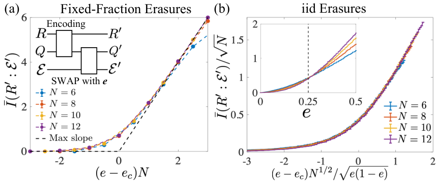
In contrast to our analysis of the stabilizer codes, we do not perform an optimal decoding analysis and only test for the existence of an erasure threshold. We consider the coherent quantum information of an initial state in the code space after application of the erasure channel in Eq. (9) on a random set of the sites
| (38) |
where is an initial encoded density matrix, and is the reduced density matrix on . We study the purified channel where a reference system is used to purify and an environment purifies the error operation [see inset to Fig. 8(a)]. In the case of the erasure error, the interaction of the system with the environment is through a SWAP operation of each erased qubit in with a qubit in . The mutual information between the reference and the fictitious environment is equal to
| (39) |
where is the rate of the code. As we discussed in Sec. III.1, when , then the max-entanglement fidelity for that input state satisfies , i.e., for sufficiently small, the error channel can be approximately decoded.
In Fig. 8, we show the results of numerical simulations for for the Haar random code with a that acts trivially on the code space. We show the results for both fixed fraction and iid erasure errors. We see consistent scaling results with the random stabilizer code: the fixed-fraction error model leads to a finite-size rounding of the transition over a region scaling as . The random fluctuations in the total number of erasures in the iid model then round out the threshold even more, producing a “critical” region of width and amplitude at .
To obtain a more direct comparison between the Haar random and random stabilizer codes, we show the average coherent quantum information of each code ensemble in Fig. 9. We see remarkably close quantitative agreement between the code performance; however, there are significant differences that appear at the critical point. In particular, in Fig. 9(b), we see that the two codes appear to be converging to substantially different values of in the large- limit of (Haar) and (Clifford). Thus, a Haar random code is slightly more optimal than a random stabilizer code in this region where the code fails. These quantitative differences in the scaling function indicate that the random stabilizer code does not necessarily saturate the performance of an optimal code, even at leading order in the large- limit. In the case of the depolarizing channel, the optimal decoding threshold for a random stabilizer code is expected to be smaller than the channel capacity limit DiVincenzo et al. 1998; Smith and Smolin 2007.

VIII Statistical mechanics mapping: domain wall pinning
In this section, we present an approximate mapping of the erasure threshold to a first-order domain-wall pinning transition in a related statistical mechanics description. This discussion applies to both Clifford and Haar models.
We consider the quenched average of the purity of a subregion
| (40) |
A natural approximation to the coherent quantum information is the difference in log-average purity of each subregion
| (41) |
Although this quantity does not have a clear significance for error correction in general systems, we expect that, for deep Haar random circuits, the fluctuations in over circuits are small enough that it is well approximated by Nahum et al. 2017; Nahum et al. 2018a; Zhou and Nahum 2019. For any constructed of local two-qubit gates distributed according a two-design, we can compute after circuit averaging using a well-studied mapping between the average purity of subregions of a dimensional random circuit to a dimensional partition function of an Ising model with certain boundary conditions at late times Nahum et al. 2018a. The condition that the initial state is mixed on the logical qubit degrees of freedom corresponds to a spin polarized bottom boundary condition on the logical qubit sites Bao et al. 2020. In this mapping, becomes the free energy cost of flipping the polarization of the top erased boundary condition in the presence of the polarized boundary condition due to the logical qubits (see Fig. 10).

The temperature of the effective Ising model is well below the transition temperature, which implies that the free energy is minimized primarily through energy minimization. Using a minimal energy surface approximation, we obtain a direct estimate for the analog of the mutual information between the reference and the environment for the log-average purity
| (42) |
where . This quantity undergoes a phase transition at the same point as the optimal erasure threshold; thus, we suspect it captures some essential features of the threshold for the optimal code. In particular, the point corresponds to a transition in the left half of Fig. 10 where the top boundary condition is no longer sufficiently strong to polarize the bulk of the system. In this case, the middle domain flips to align with the logical qubits.
Although it is clear that our codes will not be robust against erasure errors that occur during the encoding circuit, we can gain some additional insight into the breakdown of the threshold using this statistical mechanics model. In the Ising model mapping, erasures in the bulk correspond to fixing a finite density of spins in the bulk to point along the direction, which will overcome the surface pinning effect and prevent the formation of the ordered phase in the left of Fig. 10. As a result, in order to have a fault-tolerant encoding, some form of error correction should be applied during the evolution itself.
IX Conclusions
In this paper, we revisited the study of quantum error correcting codes generated by low depth random circuits. In any spatial dimension, we found that a depth random circuit is necessary and sufficient to achieve high-performance coding against erasure errors below the optimal erasure threshold, set by the channel capacity. However, in 1D, coding arbitrarily close to the optimal threshold requires a depth circuit due to the relevance of spatial randomness in errors near code capacity. The marginal dimension for high-performance, low-depth coding at capacity is 2D where spatial randomness becomes an irrelevant perturbation.
Although spatial randomness in the errors becomes irrelevant above 1D, there are still large inhomogeneities in the quality of the random code due to random circuit fluctuations. Using a simple block model, we showed that the effects of code randomness in can be mitigated through correlated coding and the use of additional ancilla qubits that effectively reduce the rate of the code. An alternative strategy, that works better in practice, is to expurgate low-weight logical operators from the code using quantum measurements. With these methods, we found that good coding becomes possible at sub-log- depths. Codes with rates near 1/2 generated by our random coding algorithms can achieve high performance at depth 4–8 in 2D for large erasure rates and block sizes of thousands of qubits.
The results in this work open up many directions for future research. To develop these codes for use on near-term devices, a more general theory of optimal decoding for Pauli error channels should be developed. Efficient optimal decoding can likely be implemented for these low-depth codes by taking advantage of their strongly local nature. For example, a brute force method is sufficient in the block encoding model with logarithmic block sizes. It will also be interesting to consider the performance of these codes in conventional threshold theorems, including strategies for achieving full fault-tolerance, e.g., as can always be achieved with concatenation.
Another promising avenue of research is to further develop the expurgation algorithm, which we used to significantly reduce the required depth to achieve successful decoding of erasure errors. It has now been well established that fault-tolerant thresholds can be significantly improved by tailoring codes to the detailed properties of the noise Tuckett et al. 2018; Tuckett et al. 2019; Tuckett et al. 2020; Bonilla Ataides et al. 2020. The expurgation algorithm provides a wide variety of additional techniques to tailor codes to specific noise models. In addition, it may be possible to further improve the expurgation by using quantum measurements that explicitly implement entanglement swapping, similar to techniques used for the measurement based preparation of the surface code states Raussendorf et al. 2005; Han et al. 2007.
As mentioned in the introduction, developing more concrete connections between the results here and measurement-induced phase transitions is also promising to explore. Unitary-measurement models that include both errors and active error correction may realize a different universality class of these transitions that might be more resilient in near-term quantum computing devices.
Acknowledgements.
We thank Steve Girvin, Pradeep Niroula, and Sarang Gopalakrishnan for helpful discussions. M.J.G and D.A.H were supported in part by the DARPA Driven and Nonequilibrium Quantum Systems (DRINQS) program. L.J acknowledges support from the ARO (W911NF-18-1-0020, W911NF-18-1-0212), ARO MURI (W911NF-16-1-0349), AFOSR MURI (FA9550-19-1-0399), DOE (DE-SC0019406), NSF (EFMA-1640959, OMA-1936118, EEC-1941583), and the Packard Foundation (2013-39273).Appendix A Max-average fidelity for random stabilizer erasure threshold
In this appendix, we prove that the max-average fidelity converges to the perfect recovery probability for the random stabilizer erasure threshold in the thermodynamic limit.
For an initial random pure state on the unencoded logical qubits at the sites for , the probability of successful error correction following the encoding by the Clifford unitary , erasure at sites , syndrome measurements with outcome , and maximum-likelihood recovery is given by
| (43) |
where is a syndrome projector for sites and is the conditional recovery operator. We include a sum over Kroenecker delta functions , where are the set of possible syndrome outcomes for . This term is nonzero only when the observed syndrome is allowed for a given , thus, it serves as a projector onto the space of allowed syndromes. The maximum possible size of is as this is the number of Pauli group elements with support only on (modulo a phase).
The precise form of depends on the encoding circuit in addition to and , therefore, it cannot be calculated in general without completely specifying . On the other hand, we can use the fact that it can be moved past the syndrome projectors by turning this into a projector onto the perfect syndrome outcome. Since it has its support entirely on , we can then cancel the product of the two recovery operators to arrive at the much simpler formula
| (44) |
Summing over syndrome measurements gives the recovery probability
| (45) | ||||
| (46) |
Here, we used the identity
| (47) |
where runs over a basis of Pauli group elements that act on sites in the subset . Since the Clifford group forms a two-design, we have the identity from random matrix theory
| (48) |
where is an average over the Haar measure on the unitary group on qubits. This formula can be used to bound the average of the second term in Eq. (45) as
| (49) | ||||
| (50) | ||||
| (51) | ||||
| (52) |
where and in Eq. (51) we used the fact that for distributed according to the Haar measure. As a result, up to corrections that decay exponentially with for any erasure rate , we find the formula for the code-averaged max-average gate fidelity
| (53) | ||||
| (54) |
This expression for is equal to from Eq. (21).
Appendix B Counting rank- matrices over
In this appendix, we reproduce the standard formula for the number of rank- matrices over . To find the formula, we first use the fact the number of matrices of rank is given by
| (55) |
because we have choices for the first row and choices for row to ensure that it is linearly independent from the first rows. When , then we have to account for linear dependence between rows of the matrix, which leads to a degeneracy that is equal to the number of -dimensional subspaces of a dimensional vector space over
| (56) |
Here, the numerator counts the total number of bases of an -dimensional subspace of a vector space of dimension and the denominator counts the number of bases for each subspace of dimension . The number of matrices of rank is given by the product of Eq. (55) and Eq. (56)
| (57) |
Appendix C Independent-identically distributed erasure errors
In this appendix, we derive the leading order RMT solution for the recovery probability for independent-identically distributed (iid) erasure errors with error rate . As noted in Sec. II.2, the failure probability for iid errors can be obtained from the failure probability for the fixed-fraction model with . After averaging over all possible , there is additional rounding of the transition due to Poisson fluctuations in the total number of erasures. To evaluate the associated finite-size scaling, we make use of the fact that the total number of erasures is an extensive variable whose fluctuations are governed by the central limit theorem
| (58) |
In averaging over the erasure errors, we can ignore the critical region for fixed because it has a width that is much less than the typical fluctuations in
| (59) |
where and . After introducing the scaling variable , we find
| (60) | ||||
| (61) |
where is the complementary error function and is the scaling function for this random code transition. At the critical point, . This analysis implies that the critical region after averaging over has a width scaling as that arises from the width of the probability distribution of . Similarly, the average log-failure probability at the critical erasure rate scales as .
Appendix D Self-averaging of random stabilizer code transition
One of the central assumptions in this work is that the finite-size scaling behavior of random stabilizer codes near threshold well approximates the behavior of the optimal codes.
A necessary condition for this to be true is that the random codes are self-averaging in the sense that a single realization of a random code has the same properties as the average over codes in the large limit.
To test this self-averaging condition, we investigate the convergence with towards the RMT prediction for the critical recovery probability for single realizations.
Numerical Monte Carlo results for the standard deviation are shown in Fig. 11.
We fix a random Clifford unitary generated by a high-depth circuit (depth in 1D).
For that circuit, we then estimate at the critical point of the optimal codes for the fixed-fraction erasure model.
By generating many codes, we can then estimate the variance through sampling.
Over the range of sizes shown in the figure, we see clear exponential decay of the standard deviation with , indicating that self-averages to the RMT prediction in the large limit.
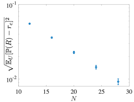
References
- Arute et al. (2019) F. Arute, K. Arya, R. Babbush, D. Bacon, J. C. Bardin, R. Barends, R. Biswas, S. Boixo, F. G. S. L. Brandao, D. A. Buell, et al., Quantum supremacy using a programmable superconducting processor, Nature 574, 505 (2019).
- Gaebler et al. (2016) J. P. Gaebler, T. R. Tan, Y. Lin, Y. Wan, R. Bowler, A. C. Keith, S. Glancy, K. Coakley, E. Knill, D. Leibfried, et al., High-fidelity universal gate set for ion qubits, Phys. Rev. Lett. 117, 060505 (2016).
- Debnath et al. (2016) S. Debnath, N. M. Linke, C. Figgatt, K. A. Landsman, K. Wright, and C. Monroe, Demonstration of a small programmable quantum computer with atomic qubits, Nature 536, 63 (2016).
- Córcoles et al. (2015) A. D. Córcoles, E. Magesan, S. J. Srinivasan, A. W. Cross, M. Steffen, J. M. Gambetta, and J. M. Chow, Demonstration of a quantum error detection code using a square lattice of four superconducting qubits, Nature Communications 6, 2152 (2015).
- Ofek et al. (2016) N. Ofek, A. Petrenko, R. Heeres, P. Reinhold, Z. Leghtas, B. Vlastakis, Y. Liu, L. Frunzio, S. M. Girvin, L. Jiang, et al., Extending the lifetime of a quantum bit with error correction in superconducting circuits, Nature 536, 441 (2016).
- Neill et al. (2018) C. Neill, P. Roushan, K. Kechedzhi, S. Boixo, S. V. Isakov, V. Smelyanskiy, A. Megrant, B. Chiaro, A. Dunsworth, K. Arya, et al., A blueprint for demonstrating quantum supremacy with superconducting qubits, Science 360, 195 (2018).
- Mi et al. (2018) X. Mi, M. Benito, S. Putz, D. M. Zajac, J. M. Taylor, G. Burkard, and J. R. Petta, A coherent spin–photon interface in silicon, Nature 555, 599 (2018).
- Huang et al. (2019) W. Huang, C. H. Yang, K. W. Chan, T. Tanttu, and B. Hensen, Fidelity benchmarks for two-qubit gates in silicon, Nature 569, 532 (2019).
- Levine et al. (2019) H. Levine, A. Keesling, G. Semeghini, A. Omran, T. T. Wang, S. Ebadi, H. Bernien, M. Greiner, V. Vuletić, H. Pichler, et al., Parallel Implementation of High-Fidelity Multiqubit Gates with Neutral Atoms, Phys. Rev. Lett. 123, 170503 (2019).
- Egan et al. (2020) L. Egan, D. M. Debroy, C. Noel, A. Risinger, D. Zhu, D. Biswas, M. Newman, M. Li, K. R. Brown, M. Cetina, et al., Fault-Tolerant Operation of a Quantum Error-Correction Code (2020), eprint arXiv:2009.11482.
- Knill (2005) E. Knill, Quantum computing with realistically noisy devices, Nature 434, 39 (2005).
- Bravyi and Kitaev (2005) S. Bravyi and A. Kitaev, Universal quantum computation with ideal Clifford gates and noisy ancillas, Phys. Rev. A 71, 022316 (2005).
- Svore et al. (2007) K. M. Svore, D. P. DiVincenzo, and B. M. Terhal, Noise Threshold for a Fault-Tolerant Two-Dimensional Lattice Architecture, Quant. Inf. Comp. 7, 297 (2007).
- Fowler et al. (2012) A. G. Fowler, M. Mariantoni, J. M. Martinis, and A. N. Cleland, Surface codes: Towards practical large-scale quantum computation, Phys. Rev. A 86, 032324 (2012).
- Leghtas et al. (2013) Z. Leghtas, G. Kirchmair, B. Vlastakis, R. J. Schoelkopf, M. H. Devoret, and M. Mirrahimi, Hardware-Efficient Autonomous Quantum Memory Protection, Phys. Rev. Lett. 111, 120501 (2013).
- Mirrahimi et al. (2014) M. Mirrahimi, Z. Leghtas, V. V. Albert, S. Touzard, R. J. Schoelkopf, L. Jiang, and M. H. Devoret, Dynamically protected cat-qubits: a new paradigm for universal quantum computation, New J. of Phys. 16, 045014 (2014).
- Vlastakis et al. (2013) B. Vlastakis, G. Kirchmair, Z. Leghtas, S. E. Nigg, L. Frunzio, S. M. Girvin, M. Mirrahimi, M. H. Devoret, and R. J. Schoelkopf, Deterministically Encoding Quantum Information Using 100-Photon Schrödinger Cat States, Science 342, 607 (2013).
- Martinis (2015) J. M. Martinis, Qubit metrology for building a fault-tolerant quantum computer, npj Quantum Inf 1, 1 (2015).
- Harper et al. (2020) R. Harper, S. T. Flammia, and J. J. Wallman, Efficient learning of quantum noise, Nature Phys. 332, 1 (2020).
- Flammia and Wallman (2020) S. T. Flammia and J. J. Wallman, Efficient estimation of pauli channels (2020), eprint arXiv:1907.12976.
- Aliferis and Preskill (2008) P. Aliferis and J. Preskill, Fault-tolerant quantum computation against biased noise, Phys. Rev. A 78 (2008).
- Puri et al. (2020) S. Puri, L. St-Jean, J. A. Gross, A. Grimm, N. E. Frattini, P. S. Iyer, A. Krishna, S. Touzard, L. Jiang, A. Blais, et al., Bias-preserving gates with stabilized cat qubits, Science Adv. 6, eaay5901 (2020).
- Guillaud and Mirrahimi (2019) J. Guillaud and M. Mirrahimi, Repetition cat qubits for fault-tolerant quantum computation, Phys. Rev. X 9 (2019).
- Tillich and Zemor (2009) J.-P. Tillich and G. Zemor, Quantum LDPC codes with positive rate and minimum distance proportional to (2009), eprint arXiv:0903.0566.
- Hastings (2013) M. B. Hastings, Decoding in Hyperbolic Spaces: LDPC Codes With Linear Rate and Efficient Error Correction (2013), eprint arXiv:1312.2546.
- Gottesman (2013) D. Gottesman, Fault-Tolerant Quantum Computation with Constant Overhead (2013), eprint arXiv:1310.2984.
- Tuckett et al. (2018) D. K. Tuckett, S. D. Bartlett, and S. T. Flammia, Ultrahigh error threshold for surface codes with biased noise, Phys. Rev. Lett. 120, 050505 (2018).
- Tuckett et al. (2019) D. K. Tuckett, A. S. Darmawan, C. T. Chubb, S. Bravyi, S. D. Bartlett, and S. T. Flammia, Tailoring surface codes for highly biased noise, Phys. Rev. X 9, 041031 (2019).
- Tuckett et al. (2020) D. K. Tuckett, S. D. Bartlett, S. T. Flammia, and B. J. Brown, Fault-tolerant thresholds for the surface code in excess of under biased noise, Phys. Rev. Lett. 124, 130501 (2020).
- Bonilla Ataides et al. (2020) J. P. Bonilla Ataides, D. K. Tuckett, S. D. Bartlett, S. T. Flammia, and B. J. Brown, The XZZX surface code (2020), eprint arXiv:2009.07851.
- (31) C. E. Shannon, A Mathematical Theory of Communication, Bell System Technical Journal. 27, 379 (1948).
- Gallager (1962) R. G. Gallager, Low-density parity-check codes, IRE Trans. Info. Theory 8, 21 (1962).
- Gallager (1973) R. Gallager, The random coding bound is tight for the average code, IEEE Trans. Inform. Theory IT-19, 244 (1973).
- Brown and Fawzi (2015) W. Brown and O. Fawzi, Decoupling with Random Quantum Circuits, Commun. Math. Phys. 340, 867 (2015), eprint arXiv:1210.6644.
- Brown and Fawzi (2013) W. Brown and O. Fawzi, Short random circuits define good quantum error correcting codes, Proceedings of ISIT, pages 346 - 350 (2013), eprint arXiv:1312.7646.
- Cleve et al. (2016) R. Cleve, D. Leung, L. Liu, and C. Wang, Near-linear constructions of exact unitary 2-designs, Quantum Inf. Comp. 16, 0721 (2016), eprint arXiv:1501.04592.
- Brandao et al. (2016) F. G. S. L. Brandao, A. W. Harrow, and M. Horodecki, Local Random Quantum Circuits are Approximate Polynomial-Designs, Commun. Math. Phys. 346, 397 (2016).
- Harrow and Mehraban (2018) A. Harrow and S. Mehraban, Approximate unitary -designs by short random quantum circuits using nearest-neighbor and long-range gates (2018), eprint arXiv:1809.06957.
- Delfosse et al. (2016) N. Delfosse, P. Iyer, and D. Poulin, A linear-time benchmarking tool for generalized surface codes (2016), eprint arXiv:1611.04256.
- Delfosse and Zémor (2020) N. Delfosse and G. Zémor, Linear-time maximum likelihood decoding of surface codes over the quantum erasure channel, Phys. Rev. Research 2, 033042 (2020), eprint arXiv:1703.01517.
- Imry and Ma (1975) Y. Imry and S.-k. Ma, Random-field instability of the ordered state of continuous symmetry, Phys. Rev. Lett. 35, 1399 (1975).
- Shor (1996) P. W. Shor, Fault-tolerant quantum computation (1996), eprint arxiv:quant-ph/9605011.
- Aharonov and Ben-Or (1999) D. Aharonov and M. Ben-Or, Fault-Tolerant Quantum Computation With Constant Error Rate (1999), eprint arXiv:quant-ph/9906129.
- Gottesman (2000) D. Gottesman, Fault-tolerant quantum computation with local gates, J. Mod. Opt. 47, 333 (2000).
- Kitaev (1997) A. Y. Kitaev, Quantum computations: algorithms and error correction, Russ. Math. Surv. 52, 1191 (1997).
- Dennis et al. (2002) E. Dennis, A. Kitaev, A. Landahl, and J. Preskill, Topological quantum memory, J. Math. Phys. 43, 4452 (2002).
- Chubb and Flammia (2018) C. T. Chubb and S. T. Flammia, Statistical mechanical models for quantum codes with correlated noise (2018), eprint arXiv:1809.10704.
- Duclos-Cianci and Poulin (2010) G. Duclos-Cianci and D. Poulin, Fast decoders for topological quantum codes, Phys. Rev. Lett. 104, 050504 (2010).
- Wootton and Loss (2012) J. R. Wootton and D. Loss, High threshold error correction for the surface code, Phys. Rev. Lett. 109, 160503 (2012).
- Hutter et al. (2014) A. Hutter, J. R. Wootton, and D. Loss, Efficient markov chain monte carlo algorithm for the surface code, Phys. Rev. A 89, 022326 (2014).
- Delfosse and Nickerson (2017) N. Delfosse and N. H. Nickerson, Almost-linear time decoding algorithm for topological codes (2017), eprint arXiv:1709.06218.
- Bombin and Martin-Delgado (2006) H. Bombin and M. A. Martin-Delgado, Topological quantum distillation, Phys. Rev. Lett. 97, 180501 (2006).
- Bombin and Martin-Delgado (2007) H. Bombin and M. A. Martin-Delgado, Topological computation without braiding, Phys. Rev. Lett. 98, 160502 (2007).
- Bombin (2011) H. Bombin, Clifford gates by code deformation, New J. Phys. 13, 043005 (2011).
- Horsman et al. (2012) C. Horsman, A. G. Fowler, S. Devitt, and R. Van Meter, Surface code quantum computing by lattice surgery, New J. Phys. 14, 123011 (2012).
- Brown et al. (2017) B. J. Brown, K. Laubscher, M. S. Kesselring, and J. R. Wootton, Poking holes and cutting corners to achieve clifford gates with the surface code, Phys. Rev. X 7, 021029 (2017).
- Webster and Bartlett (2020) P. Webster and S. D. Bartlett, Fault-tolerant quantum gates with defects in topological stabilizer codes, Phys. Rev. A 102, 022403 (2020).
- Brown (2020) B. J. Brown, A fault-tolerant non-Clifford gate for the surface code in two dimensions, Science Adv. 6, eaay4929 (2020).
- Bravyi et al. (2010) S. Bravyi, D. Poulin, and B. Terhal, Tradeoffs for reliable quantum information storage in 2d systems, Phys. Rev. Lett. 104, 050503 (2010).
- Bacon (2006) D. Bacon, Operator quantum error-correcting subsystems for self-correcting quantum memories, Phys. Rev. A 73, 012340 (2006).
- Leverrier et al. (2015) A. Leverrier, J.-P. Tillich, and G. Zemor, Quantum Expander Codes, 2015 IEEE 56th Annual Symposium on Foundations of Computer Science (FOCS) pp. 810–824 (2015), eprint arXiv:1504.00822.
- Bolt et al. (2018) A. Bolt, D. Poulin, and T. M. Stace, Decoding schemes for foliated sparse quantum error-correcting codes, Phys. Rev. A 98, 062302 (2018).
- Kovalev and Pryadko (2013) A. A. Kovalev and L. P. Pryadko, Fault tolerance of quantum low-density parity check codes with sublinear distance scaling, Phys. Rev. A 87, 020304 (2013).
- Fawzi et al. (2018) O. Fawzi, A. Grospellier, and A. Leverrier, Constant overhead quantum fault-tolerance with quantum expander codes (2018), eprint arXiv:1808.03821.
- Monroe et al. (2014) C. Monroe, R. Raussendorf, A. Ruthven, K. R. Brown, P. Maunz, L.-M. Duan, and J. Kim, Large-scale modular quantum-computer architecture with atomic memory and photonic interconnects, Phys. Rev. A 89, 022317 (2014).
- Landsman et al. (2019) K. A. Landsman, Y. Wu, P. H. Leung, D. Zhu, N. M. Linke, K. R. Brown, L. Duan, and C. Monroe, Two-qubit entangling gates within arbitrarily long chains of trapped ions, Phys. Rev. A 100, 022332 (2019).
- Kimble (2008) H. J. Kimble, The quantum internet, Nature 453, 1023 (2008).
- Pastawski et al. (2015) F. Pastawski, B. Yoshida, D. Harlow, and J. Preskill, Holographic quantum error-correcting codes: toy models for the bulk/boundary correspondence, J. High Energ. Phys. 2015, 163 (2015).
- Harris et al. (2018) R. J. Harris, N. A. McMahon, G. K. Brennen, and T. M. Stace, Calderbank-shor-steane holographic quantum error-correcting codes, Phys. Rev. A 98, 052301 (2018).
- Hayden and Preskill (2007) P. Hayden and J. Preskill, Black holes as mirrors: quantum information in random subsystems, J. High Energ. Phys. 2007, 120 (2007), eprint arXiv:0708.4025.
- Lashkari et al. (2013) N. Lashkari, D. Stanford, M. Hastings, T. Osborne, and P. Hayden, Towards the fast scrambling conjecture, J. High Energ. Phys. 2013, 22 (2013), eprint arXiv:1111.6580.
- Hosur et al. (2016) P. Hosur, X.-L. Qi, D. A. Roberts, and B. Yoshida, Chaos in quantum channels, J. High Energ. Phys. 2016, 4 (2016), eprint arXiv:1511.04021.
- Nahum et al. (2017) A. Nahum, J. Ruhman, S. Vijay, and J. Haah, Quantum entanglement growth under random unitary dynamics, Phys. Rev. X 7, 031016 (2017).
- Nahum et al. (2018a) A. Nahum, S. Vijay, and J. Haah, Operator spreading in random unitary circuits, Phys. Rev. X 8, 021014 (2018a).
- von Keyserlingk et al. (2018) C. W. von Keyserlingk, T. Rakovszky, F. Pollmann, and S. L. Sondhi, Operator hydrodynamics, otocs, and entanglement growth in systems without conservation laws, Phys. Rev. X 8, 021013 (2018).
- Nahum et al. (2018b) A. Nahum, J. Ruhman, and D. A. Huse, Dynamics of entanglement and transport in one-dimensional systems with quenched randomness, Phys. Rev. B 98, 035118 (2018b).
- Khemani et al. (2018) V. Khemani, A. Vishwanath, and D. A. Huse, Operator spreading and the emergence of dissipative hydrodynamics under unitary evolution with conservation laws, Phys. Rev. X 8, 031057 (2018).
- Rakovszky et al. (2018) T. Rakovszky, F. Pollmann, and C. W. von Keyserlingk, Diffusive hydrodynamics of out-of-time-ordered correlators with charge conservation, Phys. Rev. X 8, 031058 (2018).
- Chan et al. (2018) A. Chan, A. De Luca, and J. T. Chalker, Solution of a minimal model for many-body quantum chaos, Phys. Rev. X 8, 041019 (2018).
- Zhou and Nahum (2019) T. Zhou and A. Nahum, Emergent statistical mechanics of entanglement in random unitary circuits, Phys. Rev. B 99, 174205 (2019).
- Brandao and Horodecki (2013) F. G. S. L. Brandao and M. Horodecki, Exponential Quantum Speed-ups are Generic, Q. Inf. Comp. 13, 0901 (2013), eprint arXiv:1010.3654.
- Boixo et al. (2018) S. Boixo, S. V. Isakov, V. N. Smelyanskiy, R. Babbush, N. Ding, Z. Jiang, M. J. Bremner, J. M. Martinis, and H. Neven, Characterizing quantum supremacy in near-term devices, Nature Phys. 14, 595 (2018).
- Bouland et al. (2019) A. Bouland, B. Fefferman, C. Nirkhe, and U. Vazirani, On the complexity and verification of quantum random circuit sampling, Nature Phys. 15, 159 (2019).
- Movassagh (2019) R. Movassagh, Quantum supremacy and random circuits (2019), eprint arXiv:1909.06210.
- Deutsch (1991) J. M. Deutsch, Quantum statistical mechanics in a closed system, Phys. Rev. A 43, 2046 (1991).
- Srednicki (1993) M. Srednicki, Entropy and area, Phys. Rev. Lett. 71, 666 (1993).
- Nandkishore and Huse (2015) R. Nandkishore and D. A. Huse, Many-body localization and thermalization in quantum statistical mechanics, Annu. Rev. Condens. Matter Phys. 6, 15 (2015).
- D’Alessio et al. (2016) L. D’Alessio, Y. Kafri, A. Polkovnikov, and M. Rigol, From quantum chaos and eigenstate thermalization to statistical mechanics and thermodynamics, Adv. Phys. 65, 239 (2016).
- Li et al. (2018) Y. Li, X. Chen, and M. P. A. Fisher, Quantum zeno effect and the many-body entanglement transition, Phys. Rev. B 98, 205136 (2018).
- Skinner et al. (2019) B. Skinner, J. Ruhman, and A. Nahum, Measurement-induced phase transitions in the dynamics of entanglement, Phys. Rev. X 9, 031009 (2019).
- Li et al. (2019) Y. Li, X. Chen, and M. P. A. Fisher, Measurement-driven entanglement transition in hybrid quantum circuits, Phys. Rev. B 100, 134306 (2019).
- Chan et al. (2019) A. Chan, R. M. Nandkishore, M. Pretko, and G. Smith, Unitary-projective entanglement dynamics, Phys. Rev. B 99, 224307 (2019).
- Gullans and Huse (2020a) M. J. Gullans and D. A. Huse, Dynamical purification phase transition induced by quantum measurements, Phys. Rev. X 10, 041020 (2020a).
- Choi et al. (2020) S. Choi, Y. Bao, X.-L. Qi, and E. Altman, Quantum error correction in scrambling dynamics and measurement-induced phase transition, Phys. Rev. Lett. 125, 030505 (2020).
- Cao et al. (2019) X. Cao, A. Tilloy, and A. D. Luca, Entanglement in a fermion chain under continuous monitoring, SciPost Phys. 7, 24 (2019).
- Szyniszewski et al. (2019) M. Szyniszewski, A. Romito, and H. Schomerus, Entanglement transition from variable-strength weak measurements, Phys. Rev. B 100, 064204 (2019).
- Bao et al. (2020) Y. Bao, S. Choi, and E. Altman, Theory of the phase transition in random unitary circuits with measurements, Phys. Rev. B 101, 104301 (2020).
- Jian et al. (2020) C.-M. Jian, Y.-Z. You, R. Vasseur, and A. W. W. Ludwig, Measurement-induced criticality in random quantum circuits, Phys. Rev. B 101, 104302 (2020).
- Gullans and Huse (2020b) M. J. Gullans and D. A. Huse, Scalable probes of measurement-induced criticality, Phys. Rev. Lett. 125, 070606 (2020b).
- Zabalo et al. (2020) A. Zabalo, M. J. Gullans, J. H. Wilson, S. Gopalakrishnan, D. A. Huse, and J. H. Pixley, Critical properties of the measurement-induced transition in random quantum circuits, Phys. Rev. B 101, 060301 (2020).
- Zhang et al. (2020) L. Zhang, J. A. Reyes, S. Kourtis, C. Chamon, E. R. Mucciolo, and A. E. Ruckenstein, Nonuniversal entanglement level statistics in projection-driven quantum circuits, Phys. Rev. B 101, 235104 (2020).
- Tang and Zhu (2020) Q. Tang and W. Zhu, Measurement-induced phase transition: A case study in the nonintegrable model by density-matrix renormalization group calculations, Phys. Rev. Research 2, 013022 (2020).
- Li et al. (2020) Y. Li, X. Chen, A. W. W. Ludwig, and M. P. A. Fisher, Conformal invariance and quantum non-locality in hybrid quantum circuits (2020), eprint arXiv:2003.12721.
- Fuji and Ashida (2020) Y. Fuji and Y. Ashida, Measurement-induced quantum criticality under continuous monitoring, Phys. Rev. B 102, 054302 (2020).
- Lavasani et al. (2020) A. Lavasani, Y. Alavirad, and M. Barkeshli, Measurement-induced topological entanglement transitions in symmetric random quantum circuits (2020), eprint arXiv:2004.07243.
- Sang and Hsieh (2020) S. Sang and T. H. Hsieh, Measurement Protected Quantum Phases (2020), eprint arXiv:2004.09509.
- Ippoliti et al. (2020) M. Ippoliti, M. J. Gullans, S. Gopalakrishnan, D. A. Huse, and V. Khemani, Entanglement phase transitions in measurement-only dynamics (2020), eprint arXiv:2004.09560.
- Alberton et al. (2020) O. Alberton, M. Buchhold, and S. Diehl, Trajectory dependent entanglement transition in a free fermion chain – from extended criticality to area law (2020), eprint arXiv:2005.09722.
- Lunt and Pal (2020) O. Lunt and A. Pal, Measurement-induced entanglement transitions in many-body localized systems, Phys. Rev. Research 2, 043072 (2020).
- Rossini and Vicari (2020) D. Rossini and E. Vicari, Measurement-induced dynamics of many-body systems at quantum criticality, Phys. Rev. B 102, 035119 (2020).
- Goto and Danshita (2020) S. Goto and I. Danshita, Measurement-induced transitions of the entanglement scaling law in ultracold gases with controllable dissipation, Phys. Rev. A 102, 033316 (2020).
- Lopez-Piqueres et al. (2020) J. Lopez-Piqueres, B. Ware, and R. Vasseur, Mean-field entanglement transitions in random tree tensor networks, Phys. Rev. B 102, 064202 (2020).
- Shtanko et al. (2020) O. Shtanko, Y. A. Kharkov, L. P. García-Pintos, and A. V. Gorshkov, Classical Models of Entanglement in Monitored Random Circuits (2020), eprint arXiv:2004.06736.
- Vijay (2020) S. Vijay, Measurement-Driven Phase Transition within a Volume-Law Entangled Phase (2020), eprint arXiv:2005.03052.
- Lang and Büchler (2020) N. Lang and H. P. Büchler, Entanglement transition in the projective transverse field ising model, Phys. Rev. B 102, 094204 (2020).
- Nahum et al. (2020) A. Nahum, S. Roy, B. Skinner, and J. Ruhman, Measurement and entanglement phase transitions in all-to-all quantum circuits, on quantum trees, and in Landau-Ginsburg theory (2020), eprint arXiv:2009.11311.
- Fan et al. (2020) R. Fan, S. Vijay, A. Vishwanath, and Y.-Z. You, Self-Organized Error Correction in Random Unitary Circuits with Measurement (2020), eprint arXiv:2002.12385.
- Li and Fisher (2020) Y. Li and M. P. A. Fisher, Statistical Mechanics of Quantum Error-Correcting Codes (2020), eprint arXiv:2007.03822.
- Fidkowski et al. (2020) L. Fidkowski, J. Haah, and M. B. Hastings, How Dynamical Quantum Memories Forget (2020), eprint arXiv:2008.10611.
- Napp et al. (2019) J. Napp, R. L. La Placa, A. M. Dalzell, F. G. S. L. Brandao, and A. W. Harrow, Efficient classical simulation of random shallow 2D quantum circuits (2019), eprint arXiv:2001.00021.
- Hayden et al. (2007) P. Hayden, M. Horodecki, A. Winter, and J. Yard, A decoupling approach to the quantum capacity, Open Syst. Inf. Dyn. 15, 7 (2007).
- Chubb et al. (2017) C. T. Chubb, V. Y. F. Tan, and M. Tomamichel, Moderate Deviation Analysis for Classical Communication over Quantum Channels, Commun. Math. Phys. 355, 1283 (2017).
- Tomamichel et al. (2016) M. Tomamichel, M. Berta, and J. M. Renes, Quantum coding with finite resources, Nature Commun. 7, 1 (2016).
- DiVincenzo et al. (1998) D. P. DiVincenzo, P. W. Shor, and J. A. Smolin, Quantum-channel capacity of very noisy channels, Phys. Rev. A 57, 830 (1998).
- Smith and Smolin (2007) G. Smith and J. A. Smolin, Degenerate quantum codes for pauli channels, Phys. Rev. Lett. 98, 030501 (2007).
- Bennett et al. (1997) C. H. Bennett, D. P. DiVincenzo, and J. A. Smolin, Capacities of quantum erasure channels, Phys. Rev. Lett. 78, 3217 (1997).
- Harrow and Low (2009) A. W. Harrow and R. A. Low, Random Quantum Circuits are Approximate 2-designs, Commun. Math. Phys. 291, 257 (2009).
- Nielsen and Chuang (2011) M. A. Nielsen and I. L. Chuang, Quantum Computation and Quantum Information (Cambridge University Press, New York, NY, USA, 2011), 10th ed.
- Schumacher (1996) B. Schumacher, Sending entanglement through noisy quantum channels, Phys. Rev. A 54, 2614 (1996).
- Horodecki et al. (1999) M. Horodecki, P. Horodecki, and R. Horodecki, General teleportation channel, singlet fraction, and quasidistillation, Phys. Rev. A 60, 1888 (1999).
- Nielsen (2002) M. A. Nielsen, A simple formula for the average gate fidelity of a quantum dynamical operation, Phys. Lett. A 303, 249 (2002).
- Schumacher and Nielsen (1996) B. Schumacher and M. A. Nielsen, Quantum data processing and error correction, Phys. Rev. A 54, 2629 (1996).
- Schumacher and Westmoreland (2001) B. Schumacher and M. D. Westmoreland, Approximate quantum error correction (2001), eprint arXiv:quant-ph/0112106.
- Lloyd (1997) S. Lloyd, Capacity of the noisy quantum channel, Phys. Rev. A 55, 1613 (1997).
- Devetak and Shor (2005) I. Devetak and P. W. Shor, The Capacity of a Quantum Channel for Simultaneous Transmission of Classical and Quantum Information, Commun. Math. Phys. 256, 287 (2005).
- Wilde (2017) M. M. Wilde, Quantum Information Theory (Cambridge University Press, Cambridge, UK, 2017).
- Gottesman (1998) D. Gottesman, The Heisenberg Representation of Quantum Computers (1998), eprint arXiv:quant-ph/9807006.
- Aaronson and Gottesman (2004) S. Aaronson and D. Gottesman, Improved simulation of stabilizer circuits, Phys. Rev. A 70, 052328 (2004).
- (139) See Ch. 7 of lecture notes by J. Preskill.
- Abdel-Ghaffar (2012) K. A. S. Abdel-Ghaffar, Counting matrices over finite fields having a given number of rows of unit weight, Linear Algebra and its Applications 436, 2665 (2012).
- Dalzell et al. (2020) A. M. Dalzell, N. Hunter-Jones, and F. G. S. L. Brandao, Random quantum circuits anti-concentrate in log depth (2020), eprint 2011.12277.
- Fisher (1984) M. E. Fisher, Walks, walls, wetting, and melting, J. Stat. Phys. 34, 667 (1984).
- Raussendorf et al. (2005) R. Raussendorf, S. Bravyi, and J. Harrington, Long-range quantum entanglement in noisy cluster states, Phys. Rev. A 71, 062313 (2005).
- Han et al. (2007) Y.-J. Han, R. Raussendorf, and L.-M. Duan, Scheme for demonstration of fractional statistics of anyons in an exactly solvable model, Phys. Rev. Lett. 98, 150404 (2007).