Isoperimetric properties of condenser capacity

Hyperbolic geometry. [GM, Be] For $x,y\in\mathbb{D}$ the hyperbolic distance $\rho_{\mathbb{D}}(x,y)$ is defined by

The main property of the hyperbolic distance is the invariance under the Möbius automorphisms of the unit disk $\mathbb{D}$ of the form

These transformations preserve hyperbolic length and area. In the metric space $(\mathbb{D},\rho_{\mathbb{D}})$ one can build a non-euclidean geometry, where the parallel axiom does not hold. In this geometry, usually called the hyperbolic geometry of the Poincare disk, lines are circular arcs perpendicular to the boundary $\partial\mathbb{D}\,.$ Many results of Euclidean geometry and trigonometry have counterparts in the hyperbolic geometry [Be].

Let $G$ be a Jordan domain in the plane. One can define the hyperbolic metric on $G$ in terms of the conformal Riemann mapping function $h:G\to\mathbb{D}=h(G)$ as follows:

This definition yields a well-defined metric, independent of the conformal mapping $h\,$ [Be, KL]. In hyperbolic geometry the boundary $\partial G$ has the same role as the point of $\{\infty\}$ in Euclidean geometry: both are like “horizon", we cannot see beyond it.

Hyperbolic disks. We use the notation

for the hyperbolic disk centered at $x\in\mathbb{D}$ with radius $M>0\,.$ It is a basic fact that they are Euclidean disks with the center and radius given by [HKV, p.56, (4.20)]

Note the special case $x=0$,

Capacity of a ring domain. A ring domain $D$ has two complementary components, compact sets $E$ and $F$ such that $D=\mathbb{C}\setminus(E\cup F).$ It can be understood as a condenser $(D\cup E,E)\,.$ In particular, the capacity of the annulus $\{z\in\mathbb{C}:a<|z|<b\}$ is given by [AVV], [HKV, (7.3)]

Another ring domain with known capacity is the Grötzsch ring or condenser $(\mathbb{D},[0,r]),0<r<1\,.$ Its capacity can be expressed in terms of the complete elliptic integral $\mathcal{K}(r)$ as follows [AVV]. First define the decreasing homeomorphism $\mu:(0,1]\rightarrow[0,\infty)$ by

for $r\in(0,1)\,,\,\mu(1)=0\,$. Now the Grötzsch capacity can be expressed as follows [HKV, p.122, (7.18)]

Domain functionals and extremal problems. Numerical charateristics of geometric configurations are often studied in terms of domain functionals. In this paper we study condensers and their capacities in terms of area and perimeter. The book of Polya and Szegö [PS] studies a large spectrum of these problems and many later researcher have continued their work. See the books of C. Bandle [B] and Kesavan [KES] for isoperimetric problems and A. Baernstein [BAE] and V.N. Dubinin[Du] for classical analysis and geometric function theory. In addition, the papers Sarvas [SAR], Brock-Solynin [BS], and Betsakos [Bet] should be mentioned.

The condenser capacity is invariant under conformal mapping. Therefore it is a natural idea to express the domain functionals in terms of conformally invariant geometry. There are various results for condenser capacity which reflect this invariance, but we have not seen a systematic study based on these ideas.

We study condensers of the form $(\mathbb{D},E)$ where $E$ is a compact set. In this case we use the hyperbolic geometry to define domain functionals. Our initial point is to record the relevant data [Be, p.132, Thm 7.2.2] for the above two explicitly known cases, for the condensers $(\mathbb{D},E_{j})$ with $j=1,2$ where $E_{1}=\overline{B}_{\rho}(0,M)$ and $E_{2}=[0,{\,\textnormal{th}}(M/2)]\,.$ We consider $E_{2}$ as a degenerate, extremely thin rectangle and therefore take its perimeter to be equal to $2M$ which is twice its hyperbolic diameter $M=\rho(0,{\,\textnormal{th}}(M/2))$.

Now consider a disk $E_{1}=\overline{B}_{\rho}(0,M_{1})$ and a segment $E_{2}=[0,{\,\textnormal{th}}(M_{2}/2)]$ (we consider $E_{2}$ as a very thin rectangle) with the same hyperbolic perimeter $c$. Then

Hence, by (2.7),

and, by (2.8),

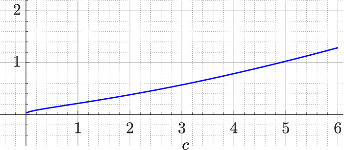
Figure 1 shows that for a fixed value of the hyperbolic perimeter $c>0\,,$ disks have larger capacity than very thin rectangles of the same hyperbolic perimeter, in other words $f_{1}(c)>f_{2}(c)$ for all $c>0\,.$ This conclusion led us to discover the following, apparently new, inequality for the special function $\mu$

In the following sections we will study variations of this theme for hyperbolic triangles and polygons.

Modulus of a curve family. For the reader’s convenience we summarize some basic facts about the moduli of curve families and their relation to capacities from the well-known sources [Ah, Du, GM, HKV, LV]. Let $\Gamma$ be a family of curves in $\mathbb{R}^{n}$. By ${\mathcal{A}}(\Gamma)$ we denote the family of admissible functions, i.e. non–negative Borel–measurable functions $\rho\,:\,\mathbb{R}^{n}\to\mathbb{R}\cup\{\infty\}$ such that

for each locally rectifiable curve $\gamma$ in $\Gamma$. For $p\geq 1$ the $p$–modulus of $\Gamma$ is defined by

where $m$ stands for the $n$–dimensional Lebesgue measure. If ${\mathcal{A}}(\Gamma)=\emptyset$, we set $\mathsf{M}_{p}(\Gamma)=\infty$. The case ${\mathcal{A}}(\Gamma)=\emptyset$ occurs only if there is a constant path in $\Gamma$ because otherwise the constant function $\infty$ is in ${\mathcal{A}}(\Gamma)$. Usually $p=n,n=2,$ and we denote $\mathsf{M}_{n}(\Gamma)$ also by $\mathsf{M}(\Gamma)$ and call it the modulus of $\Gamma$.

Numerical computing of the capacity. A numerical method for computing the capacity of condensers for doubly connected domains is presented in [NV]. The method is based on using the boundary integral equation with the generalized Neumann kernel [N1, WN]. A fast numerical method for solving the integral equation is presented in [N2] which makes use of the Fast Multipole Method toolbox [GG].

Let $G$ be a bounded simply connected domain and $E$ be a compact set in $G$ such that $D=G\setminus E$ is a doubly connected domain. Then, there exists a conformal mapping $w=f(z)$ which maps $D$ onto the annulus $\{w\,:\,q<|w|<1\}$ where $q$ is an undetermined real constant depending on $D$. The conformal mapping can be uniquely determined by assuming that $f(\alpha)>0$ for a given point $\alpha$ in $D$ (see Figure 2). Since capacity is invariant under conformal mapping, the formula (2.7) implies that

In this paper, we shall use the MATLAB function annq from [NV] to compute $\mathrm{cap}(G,E)$ where the boundary components of $D=G\setminus E$ are assumed to be piecewise smooth Jordan curves. We denote the external boundary component of $D$ by $\Gamma_{1}$ and the inner boundary component by $\Gamma_{2}$. These boundary components are oriented such that, when we proceed along the boundary $\Gamma_{1}\cup\Gamma_{2}$, the domain $D$ is always on the left side. To use the function annq, we parametrize each boundary component $\Gamma_{j}$ by a $2\pi$-periodic complex function $\eta_{j}(\delta_{j}(t))$, $t\in[0,2\pi]$, where $\delta_{j}\,:\,[0,2\pi]\to[0,2\pi]$ is a bijective strictly monotonically increasing function, $j=1,2$. When $\Gamma_{j}$ is smooth, we choose $\delta_{j}(t)=1$. For piecewise smooth boundary component $\Gamma_{j}$, the function $\delta_{j}$ is chosen as described in [LSN, p. 697]. We define $n$ equidistant nodes $s_{1},\ldots,s_{n}$ in the interval $[0,2\pi]$ by

where $n$ is an even integer. In MATLAB, we compute the vectors et and etp by

where ${\bf s}=[s_{1},\ldots,s_{n}]\in\mathbb{R}^{n}$. Then the capacity of the condenser $(G,E)$ is computed by calling

  [˜,cap] = annq(et,etp,n,alpha,z2,’b’),

where $z_{2}$ is an auxiliary point in $E$, i.e., $z_{2}$ is chosen in the domain bounded by $\Gamma_{2}$ (See Figure 2). For more details, we refer the reader to [NV]. The codes for all presented computations in this paper are available in the link https://github.com/mmsnasser/iso.

Hyperbolic triangle. First, we consider condensers of the form $(\mathbb{D},T)$ where $T$ is a closed hyperbolic triangle with vertices $s_{1},s_{2},s_{3}\in\mathbb{D}\,.$ The sides of $T$ are subarcs of circles orthogonal to $\partial\mathbb{D}\,,$ each subarc joining two vertices. Denote the the angles at vertices $s_{1},s_{2},s_{3}$ by $\sigma_{1},\sigma_{2},\sigma_{3}\,,$ respectively. Then the hyperbolic area of $T$ is given by [Be, p. 150, Thm 7.13.1]

It is a basic fact that $\mbox{h-area}(T)$ is invariant under Möbius transformations of $\mathbb{D}\,$ onto itself. Also the capacity of the condenser $(\mathbb{D},T)$ has the same invariance property.

Motivated by the simple fact that symmetry is often connected with extremal problems, we arrived at the following conjecture.

By Möbius invariance we may without loss of generality normalize $T_{0}$ as follows. Write $\omega=(\sigma_{1}+\sigma_{2}+\sigma_{3})/3\,.$ If $A,B,C$ are the lengths of the sides opposite to the angles $\sigma_{1},\sigma_{2},\sigma_{3}\,,$ resp., then by [Be, p.150, Ex. 7.12(2)] the triangle is equilateral iff $\sigma_{1}=\sigma_{2}=\sigma_{3}=\omega$ and

We may assume also that

By [Be, p. 40] we have

and solving this for $r^{2}$ we obtain

These observations show that given a hyperbolic triangle $T$ with angles $\sigma_{1},\sigma_{2},\sigma_{3}\,,$ there is a hyperbolic triangle $T_{0}$ with vertices

where $r^{2}$ is given by (3.7) with $\omega=(\sigma_{1}+\sigma_{2}+\sigma_{3})/3$. Both hyperbolic triangles $T$ and $T_{0}$ have the same hyperbolic area.

We compute $\mathrm{cap}(\mathbb{D},T)$ numerically using the MATLAB function annq with $n=3\times 10^{12}$ where the domain $D$ is the bounded doubly connected domain in the interior of the unit circle and in the exterior of the triangle (see Figure 3 where the auxiliary points $\alpha$ and $z_{2}$ in annq are shown as the star and the dot, respectively). The values of $\mathrm{cap}(\mathbb{D},T_{0})$ are computed similarly. The approximate values of the capacities $\mathrm{cap}(\mathbb{D},T)$ and $\mathrm{cap}(\mathbb{D},T_{0})$ for several values of $s_{1}$, $s_{2}$, and $s_{3}$ are presented in Table 2. The presented numerical results validate the conjectural inequality (3.5). Numerical experiments for several other values $s_{1}$, $s_{2}$, and $s_{3}$ (not presented here) also validate the conjectural inequality (3.5).

References

• [Ah] L.V. Ahlfors: Conformal invariants. McGraw-Hill, New York, 1973.
• [AVV] G. D. Anderson, M. K. Vamanamurthy, and M. Vuorinen: Conformal invariants, inequalities and quasiconformal maps. J. Wiley, 1997.
• [BAE] A. Baernstein: Symmetrization in analysis. With David Drasin and Richard S. Laugesen. With a foreword by Walter Hayman. New Mathematical Monographs, 36. Cambridge University Press, Cambridge, 2019. xviii+473 pp.
• [B] C. Bandle: Isoperimetric inequalities and applications. Monographs and Studies in Mathematics, 7. Pitman (Advanced Publishing Program), Boston, Mass.-London, 1980. x+228 pp.
• [Be] A. F. Beardon: The geometry of discrete groups. Graduate texts in Math., Vol. 91, Springer-Verlag, New York, 1983.
• [Bet] D. Betsakos: Geometric versions of Schwarz’s lemma for quasiregular mappings. Proc. Amer. Math. Soc. 139 (2011), no. 4, 1397–1407.
• [BSV] D. Betsakos, K. Samuelsson, and M. Vuorinen: The computation of capacity of planar condensers. Publ. Inst. Math. (Beograd) (N.S.) 75(89) (2004), 233–252.
• [BV] D. Betsakos and M. Vuorinen : Estimates for conformal capacity. Constr. Approx. 16 (2000), no. 4, 589–602.
• [BBG] S. Bezrodnykh, A. Bogatyrev, S. Goreinov, O. Grigoriev, H. Hakula, and M. Vuorinen: On capacity computation for symmetric polygonal condensers. J. Comput. Appl. Math. 361 (2019), 271–282.
• [BCH] C. Bianchini, G. Croce, and A. Henrot: On the quantitative isoperimetric inequality in the plane with the barycentric distance. arXiv 1904.02759
• [BS] F. Brock and A.Yu. Solynin: An approach to symmetrization via polarization. (English summary) Trans. Amer. Math. Soc. 352 (2000), no. 4, 1759–1796.
• [DMM] G.De Philippis, M. Marini, and E. Mukoseeva: The sharp quantitative isocapacitary inequality. arXiv 1901.11309
• [Du] V. N. Dubinin: Condenser Capacities and Symmetrization in Geometric Function Theory, Birkhäuser, 2014.
• [GM] J.B. Garnett and D.E. Marshall: Harmonic measure. Reprint of the 2005 original. New Mathematical Monographs, 2. Cambridge University Press, Cambridge, 2008. xvi+571 pp.
• [G] F.W. Gehring: Inequalities for condensers, hyperbolic capacity, and extremal lengths. Michigan Math. J. 18 (1971), 1–20.
• [GG] L. Greengard and Z. Gimbutas: FMMLIB2D: A MATLAB toolbox for fast multipole method in two dimensions. Version 1.2, http://www.cims.nyu.edu/cmcl/fmm2dlib/fmm2dlib.html. Accessed 1 Jan 2018.
• [HKV] P. Hariri, R. Klén and M. Vuorinen: Conformally invariant metrics and quasiconformal mappings. Springer Monographs in Mathematics, Springer, 2020.
• [J] J.A. Jenkins: Univalent functions and conformal mapping. Springer-Verlag Berlin Heidelberg, 1958.
• [KL] L. Keen and N. Lakic: Hyperbolic geometry from a local viewpoint. London Mathematical Society Student Texts, 68. Cambridge University Press, Cambridge, 2007. x+271 pp
• [KES] S. Kesavan: Symmetrization & applications. Series in Analysis, 3. World Scientific Publishing Co. Pte. Ltd., Hackensack, NJ, 2006. xii+148 pp.
• [LV] O. Lehto and K.I. Virtanen: Quasiconformal mappings in the plane, 2nd edition, Springer, Berlin, 1973.
• [LSN] J. Liesen, O. Séte and M.M.S. Nasser: Fast and accurate computation of the logarithmic capacity of compact sets. Comput. Methods Funct. Theory 17 (2017), 689–713.
• [N1] M.M.S. Nasser: Numerical conformal mapping via a boundary integral equation with the generalized Neumann kernel. SIAM J. Sci. Comput. 31 (2009), 1695–1715.
• [N2] M.M.S. Nasser: Fast solution of boundary integral equations with the generalized Neumann kernel. Electron. Trans. Numer. Anal. 44 (2015), 189–229.
• [NV] M.M.S. Nasser and M. Vuorinen: Computation of conformal invariants. Appl. Math. Comput. 389 (2021), 125617.
• [PS] G. Pólya and G. Szegö: Isoperimetric Inequalities in Mathematical Physics. Annals of Mathematics Studies, no. 27, Princeton University Press, Princeton, N. J., 1951. xvi+279 pp
• [SAR] J. Sarvas: Symmetrization of condensers in n-space. Ann. Acad. Sci. Fenn. Ser. A. I. 1972, no. 522, 44 pp.
• [SL] R. Schinzinger and P. A. A. Laura: Conformal mapping. Methods and applications. Revised edition of the 1991 original. Dover Publications, Inc., Mineola, NY, 2003. xxiv+583 pp.
• [SO1] A. Yu. Solynin: Solution of the Pólya-Szegö isoperimetric problem. (Russian) Zap. Nauchn. Sem. Leningrad. Otdel. Mat. Inst. Steklov. (LOMI) 168 (1988), Anal. Teor. Chisel i Teor. Funktsii. 9, 140–153, 190; translation in J. Soviet Math. 53 (1991), no. 3, 311–320.
• [SO2] A. Yu. Solynin: Some extremal problems on the hyperbolic polygons. Complex Variables Theory Appl. 36 (1998), no. 3, 207–231.
• [SOZ] A. Yu. Solynin and V.A. Zalgaller: An isoperimetric inequality for logarithmic capacity of polygons. Ann. of Math. (2) 159 (2004), no. 1, 277–303.
• [VA] A. Vasil’ev: Moduli of Families of Curves for Conformal and Quasiconformal Mappings. Springer-Verlag, Berlin, 2002.
• [V] M. Vuorinen: Conformal geometry and quasiregular mappings. Lecture Notes in Mathematics, 1319. Springer-Verlag, Berlin, 1988. xx+209 pp.
• [WN] R. Wegmann and M.M.S. Nasser: The Riemann-Hilbert problem and the generalized Neumann kernel on multiply connected regions. J. Comput. Appl. Math. 214 (2008), 36–57.