An Introduction to Electrocatalyst Design using Machine Learning
for Renewable Energy Storage
Abstract
Scalable and cost-effective solutions to renewable energy storage are essential to addressing the world’s rising energy needs while reducing climate change. As we increase our reliance on renewable energy sources such as wind and solar, which produce intermittent power, storage is needed to transfer power from times of peak generation to peak demand. This may require the storage of power for hours, days, or months. One solution that offers the potential of scaling to nation-sized grids is the conversion of renewable energy to other fuels, such as hydrogen or methane. To be widely adopted, this process requires cost-effective solutions to running electrochemical reactions. An open challenge is finding low-cost electrocatalysts to drive these reactions at high rates. Through the use of quantum mechanical simulations (density functional theory), new catalyst structures can be tested and evaluated. Unfortunately, the high computational cost of these simulations limits the number of structures that may be tested. The use of machine learning may provide a method to efficiently approximate these calculations, leading to new approaches in finding effective electrocatalysts. In this paper, we provide an introduction to the challenges in finding suitable electrocatalysts, how machine learning may be applied to the problem, and the use of the Open Catalyst Project OC20 dataset for model training.
1 Introduction
The increased use of renewable energy is essential for addressing the world’s rising energy needs while reducing climate change. Currently, renewable energy such as solar, wind and hydro generates of the US’s and of the world’s electricity EPM-US; IEO-Int. While hydro accounts for of this generation, it is limited in its ability to expand further due to resource availability and environmental concerns. Meanwhile, solar and wind are projected by 2050 to expand significantly and account for over of renewable energy generation IEO-Int. With this expansion, a unique and potentially limiting challenge arises. Unlike traditional power sources, such as coal, natural gas, and nuclear, power provided by solar and wind is intermittent.
The wind does not always blow, and the sun sets. During these periods, wind and solar plants do not generate any power. Notably, energy demand typically peaks in the early mornings (8am) and evenings (6-7pm) well outside the peak generating time (noon) for solar power power_monitor, Figure 1. On the other hand, during peak mid-day solar power generation, the power from other more conventional sources must be reduced to balance supply and demand. Adjustments in output from conventional plants may not always be able to match the variability of solar and wind power generation (e.g. due to the unpredictability of rapid weather fluctuations), resulting in an excess of supply and wasted energy cochran2014flexibility. Without further advances, it is estimated the overall penetration of solar power is capped at and costs start to rise after penetration Sivaram19. Currently, areas such as California that generate to of their power from solar CA_solar_CEC; CA_solar_SEIA are approaching these levels.

The challenges raised by intermittent power can be addressed through several means, including demand response Load_Flex; DR, improved power transmission Transmission_Madrigal, and energy storageamrouche2016overview; auer2012state; 2018iv; Renewable_Storage; ziegler2019storage. Demand response provides electricity consumers with the ability to shift power demand to time periods with high supply. The transmission of power across large distances can help both transmit power from renewable energy sites that are far away from cities, and smooth fluctuations in the generation of intermittent power by combining multiple sites. While both of these techniques are part of the solution, efficient storage of renewable energy is essential to unlocking the full potential of intermittent renewable energy.
Numerous storage techniques exist, including pumping water uphill (Pumped-Storage Hydroelectricity, PSH) Hydropower, batteries amrouche2016overview, and Hydrogen Energy Storage (HES) zhang2016survey; pickard2012addressing; Lohner2013. HES combines electricity from renewable sources with water to generate hydrogen through a process called electrolysis. The hydrogen is stored and used when needed to generate electricity through fuel cells. As described in greater detail in Section 2, each of these storage approaches has trade offs and the appropriate choice is based on the application. PSH and batteries both have high efficiency, but do not scale to the energy storage needs of large grids powered by intermittent renewable energy due to land restrictions (PSH) or cost (batteries). Hydrogen energy storage offers a unique combination of scalability, long-term storage and portability. Specifically, HES can store vast quantities of energy cheaply in the form of hydrogen using the existing gas storage infrastructure. However, other costs associated with HES has limited the adoption of this otherwise very promising technology.
Hydrogen energy storage’s high costs result from its relatively low efficiency and the capital costs associated with systems for power conversion (electricity to hydrogen and back to electricity) steward2009lifecycle; zakeri2015electrical. The efficiency of HES is estimated to be for round-trip AC to AC zakeri2015electrical, and unlikely to exceed . Compared to other systems such as PSH, which can achieve efficiency, the cost of the electricity used to feed the system is nearly double. Thus the relative overall cost of HES compared to other systems is highly dependent on fluctuations in electricity pricing. Assuming the cost of electricity from renewable energy sources continues to decline (solar costs have reduced 100-fold since 1976 owidrenewableenergy) and as the economic necessity of carbon neutral energy sources increases, the attractiveness of HES use should only improve.

The power conversion systems for HES involve splitting water into its constituent parts (hydrogen and oxygen) using an electrolyzer and converting the hydrogen back to electricity using fuel cells or other methods such as gas-fired turbines and engines (Figure 2). The electrolyzer and the fuel cell perform inverse reactions, and respectively. Both of these systems rely on materials called electrocatalyst s to increase the rate and efficiency of their respective electrochemical reactions. Unfortunately, common state-of-the-art electrocatalysts use expensive noble metals such as iridium and platinum sapountzi2017electrocatalysts. A major challenge is finding low-cost, efficient, and durable electrocatalysts for use in these reactions. If such catalysts can be found, earlier adoption of HES systems could be achieved due to significant cost reductions.
Modern design of catalyst s uses computational simulation to determine if a material is suitable for further exploration. The simulation models the interaction of a molecule with an catalyst’s surface in a process called adsorption. The adsorbed molecules—i.e., adsorbates—are typically the key chemical species involved in the chemical reactions of interest, such as OH, , or . The simulation is performed using Density Functional Theory (DFT) sholl2011density; parr1980density. While the foundations of DFT were first introduced in the 1960s hohenberg1964inhomogeneous; kohn1965self, it wasn’t until the 1990s that advances resulted in practical predictions for quantum chemistry becke2014perspective. Now DFT is commonly used to compute the interactions of atoms using a process colloquially called “relaxation”. In relaxations, DFT combines the locations of the atomic nuclei with quantum mechanics to predict the energy of the system and the forces acting on each atom. The locations of the atomic nuclei are then updated to minimize the energy, consequently changing the electronic distributions and energies. This iterative process continues until the energy of the system reaches a local minima. By examining the energy of the resulting relaxed system (system with lowest energy), we can gain insight into the overall efficiency of the reaction, i.e., how much energy results from or is needed to drive the reaction. Unfortunately, the DFT computation is extremely expensive and scales with the number of electrons in the system, which can range from O(100) to over O(5,000) electrons in practice. The result is computations that take hours or days per relaxation on O(10–100) core CPUs. Beyond DFT, alternative approaches to modeling quantum mechanics include the use of Coupled Cluster Single Double Triple (CCSDT)noga1987full that improves on the accuracy of DFT but is rarely used in practice due to its even higher computational cost, and force fields which are computationally very efficient but fall short in accuracy van2001reaxff; cornell1995second.
To enable large-scale exploration of new catalysts, efficient computational approximations to DFT are needed. One particularly promising approach is to use machine learning brockherde2017bypassing. Given a training dataset of DFT calculations, machine learning techniques, such as Deep Learning (DL), have shown the ability to learn good approximations for certain problems. These techniques take as input the state of the system, including the atom positions, element types, bond information, etc., and predict system properties such as their energy gilmer2017neural; schutt2017schnet; jorgensen2018neural; xie2018crystal. Popular datasets for this task include QM9 ramakrishnan2014quantum containing over 134k small organic molecules, the Material Project containing 70k inorganic compounds jain2013commentary, and ISO17 containing motion trajectories for 129 molecules from QM9 schutt2017schnet. Unfortunately, similar datasets relevant to our problem of interest remain limitedtran2018active; tran2019methods.
An ideal dataset containing catalysts for renewable energy storage would have two main properties. First, it would be large scale, containing DFT simulations of relevant catalysts and adsorbates. Second, the dataset would enable the training of models that take as input rough initial starting positions of the system’s atoms from which the relaxed geometries and energies could be computed. The large majority of DFT calculations are spent in the iterative computation of relaxed geometries, so efficient approximations of this process are needed. This paper provides an introduction to how the Open Catalyst Project OC20 OCD1M20 dataset addresses this task and how to apply it to training ML models.
If efficient approximations of DFT calculations can be performed, it opens the door to large scale exploration of new catalysts. Assuming catalysts are created from up to three of forty potential metals, over 10k combinations exist. Since each set of metals can be combined in various ratios and configurations, the total number of possibilities increases ad infinitum. As discussed in Section 3, determining whether a potential catalyst may be effective requires simulating its interaction with the set of potential adsorbates at all potential surfaces and binding sites. This results in O(1,000) potential simulations per catalyst. The result is a search space containing millions of possibilities requiring billions of simulations to explore! While this may seem overwhelming, with efficient DFT approximations it may be possible to compute all of them through brute force. The most promising candidates may then be verified through traditional DFT calculations before further exploration into their real-world feasibility.
While the discussion so far has focused on HES, efficient DFT approximations could be applied to numerous high-impact problems. Two notable examples include methanation and the production of ammonia fertilizer. Methanation refers to the reaction of carbon dioxide and hydrogen (generated as we described above using renewable energy) to form methane and water. Instead of storing renewable energy in the form of hydrogen this would allow storing it as methane, while having the beneficial side effect of reducing carbon dioxide (Figure 2). The potential end result could be a high density, carbon neutral fuel that fits into the current energy infrastructure sterner2009bioenergy. More complex hydrocarbon fuels beyond methane, such as ethanol, may also be created through the family of Fischer-Tropsch chemical reactions. The production of ammonia, a key ingredient in agricultural fertilizer, combines hydrogen and nitrogen to create ammonia. Currently this energy intensive process, called the Haber-Bosch process, accounts for approximately of the world’s emissions epa2016inventory. This could be greatly reduced by using renewable energy to produce the input hydrogen and by finding a more efficient reaction to Haber-Bosch.
1.1 Overview
We hope this paper serves as a gentle introduction for the machine learning community to opportunities presented by the problem of renewable energy storage, and the use of efficient ML models for atomic simulations. For researchers only interested in using the OC20 dataset for model training, Sections 2 and 3 may be skipped, and you may proceed directly to Section 4.
We begin by providing a brief overview of renewable energy storage technologies (Sec. 2) followed by an introduction to the design of catalysts using DFT (Sec. 3). We explore applications for deep learning starting in Section 4. This includes the OC20 dataset needed for training the relevant tasks (Sec. 4.1) and potential directions for ML models to addressing these tasks (Sec. ). Finally, future directions are explored in Section .
| US Power Grid 2018 | |||
| Source | Capacity (GW) | Generation (TWh) | |
| Natural Gas | 537 | 1,469 | 35.2 |
| Coal | 264 | 1,146 | 27.5 |
| Nuclear | 104 | 807 | 19.3 |
| Hydroelectric | 80 | 293 | 7.0 |
| Wind | 95 | 273 | 6.5 |
| Solar | 32 | 64 | 1.5 |
| Other | 84 | 122 | 3.0 |
| Total | 1,196 | 4,174 | – |
2 Renewable Energy Storage
In this section, we provide a brief overview of the two most popular renewable energy storage technologies—pumped-storage hydroelectricity and batteries—as well as the technologies relevant to this paper: hydrogen energy storage and methane synthesis. A summary of these technologies is provided in Table 2. For a more thorough discussion of the numerous technologies available please see amrouche2016overview; auer2012state; 2018iv; Renewable_Storage. Due to the readily available information provided by the US Energy Information Administration, we use the US as an example for our discussion below. However, results will vary by country based on geography, natural resources available, etc.
During this discussion we use the terms gigawatts (GW) and terawatt hours (TWh) (1 TW = 1,000 GW). A GW is a unit of measurement for electric capacity, i.e., how much electricity can flow at an instance in time. A TWh is a unit of electric energy, i.e., how much electricity was generated in one hour. A GW is equal to one billion watts and a TWh is equal to one trillion watt hours. For instance, a 50 GW plant operating for 1,000 hours at peak capacity would generate 50 TWh of energy. For reference, the largest nuclear power plant (Palo Verde) in the US has a capacity of 4 GW, while the average natural gas plant has 0.5 GW of capacity. In 2018, the US had a maximum capacity of 1,196 GW and generated 4,174 TWh of energy EPA-US. The percentage of actual energy produced compared to the maximum capacity (known as the capacity factor) is on average . A summary of US power generation by source is provided in Table 1.
2.1 Estimating Needed Storage Capacity
Estimating the total stored energy and capacity needed to move to renewable sources is difficult and depends on numerous factors ziegler2019storage; pump-up; nation_battery. For illustration, we consider a case where the US experiences a week of cloudy weather in the southwest and low winds in the plains. Let’s assume that during this period of the US energy would need to come from storage. In this case, 56 TWh of energy storage would be needed (4,174 TWh / year x 0.02 years x ) with a capacity of 420 GW (1.25 peak to mean ratio x 56 TWh / 168 hours per week). However, this assumes we’re only replacing energy that is currently being supplied through electricity. When including other energy sources such as gasoline powered engines and heating, the US actually uses TWh in total energy MER-US. Since electric motors are more efficient than internal combustion engines, we could potentially drop this amount by a third to 20,000 TWh. Therefore, to meet of our total energy needs over 7 days with storage, we would need roughly 250 TWh of storage and 2,000 GW of capacity. Note, these numbers should only be used as very rough guides, but provide an approximate “order of magnitude” estimate (Table 2) for our discussion below.
| Energy Storage Techniques | |||||
|---|---|---|---|---|---|
| Source | Capacity (GW) | Generation (TWh) | AC to AC Efficiency | Scale to Capacity? | Scale to Storage? |
| Pumped-Storage Hydroelectricity | 23 | 24 | No | No | |
| Batteries | 1 | 1 | Maybe | No | |
| Hydrogen Energy Storage | 0 | 0 | Maybe | Yes | |
| Methane Synthesis | 0 | 0 | Maybe | Yes | |
2.2 Pumped-Storage Hydroelectricity
Pumped-Storage Hydroelectric (PSH) refers to the conceptually simple technique of using renewable energy to pump water uphill. When additional energy is needed, the water flows back downhill through a hydroelectric plant to generate electricity. This mature technology has resulted in over 40 plants being built in the US, with most of their construction happening in the 1970s. No new plants have come online since 2012.
An advantage of PSH is their efficiency, which ranges between to for round trip AC to AC. Similar to hydroelectric plants, they are also highly responsive in that they can respond to power fluctuations in seconds. They are typically used for energy storage of 6 to 20 hours to help in system load balancing. For instance, a nuclear power plant can be kept at peak operating efficiency over 24 hours by diverting power to PSH in the night time and using hydroelectric power to meet peak demand during the daytime.
In 2018, the US PSH capacity was 23 GW EPA-US. On average, the PSH plants operated between and of full capacity depending on the time of year (more in the summer when natural water flow into reservoirs is reduced). Assuming an average of , the total energy produced by PSH is 24 TWh, or percent of the power (4,174 TWh) generated by the US in 2018.
The primary limitation of PSH is its scalability. There are not enough places to store water to meet the national energy storage needs. Current yearly generation using hydroelectric is 293 TWh with a capacity of 80 GW EPA-US, or only of the national total (Table 1). To meet the 2000 GW of capacity needed during a week of cloudy still weather, we would need to build 25 times more hydroelectric dams. This would be quite a feat, especially when all the easy to build areas are already taken. A study initiated by the US Department of Energy concluded that only 65 GW of undeveloped hydroelectric potential from streams exists in the US, which wouldn’t even double current capacity kao2014new. In another US study, it was found that if every non-hydroelectric dam was converted to hydroelectric an additional 12 GW ( of current capacity) of capacity could be created hadjerioua2012assessment. We’re also only considering capacity; this doesn’t include the infrastructure needed to pump and store the water necessary to generate 250 TWh of energy. By one estimate, the needed reservoirs’ area would be equivalent to the size of Lake Eriepump-up! Even though PSH may not grow to the scale needed for nation-sized grids, PSH remains the best option for areas that do have sufficient water storage capacity.
2.3 Batteries
When considering electricity storage technologies, batteries quickly come to mind. Battery types can vary significantly in cost, cycle life (how many times they can be discharged and recharged), energy density, and efficiency. Similar to PSH, batteries have high efficiency ( to ), which would seem to make them promising candidates for large scale energy storage. Of the numerous types that exist, the most popular include lead-acid, sodium-sulfur (NaS) and lithium-ion (Li-ion) batteries amrouche2016overview; Ogunniyi. Lead-acid batteries are relatively inexpensive and have high efficiency, but have decreased in popularity due to their lower power density and limited recharge cycles (). NaS is a promising solution for large scale systems with a greater cycle life () and low cost, but needs to operate at high temperatures (350 °C). Li-ion batteries offer a high cycle life (3,500) adachi2003development and high efficiency (). Due to the market for electric cars, the price of Li-ion batteries has decreased significantly, making them the lowest in per cycle cost. Currently, nearly all of the installed battery storage in the US uses Li-ion batteries for a combined capacity of 0.77 GW AEGR-US.
Would Li-ion batteries scale to the size of the US grid Temple; nation_battery? Recently Tesla installed a 100 MW (129 MWh) battery in Australia at a cost of $66 million. Doing the simple math, the cost of a system with 2,000 GW of capacity would be $1.23 trillion (other estimates put the cost at $2.5 trillion Temple). While this expense may be daunting, it could potentially be feasible to meet capacity demands. However, it becomes prohibitive if we consider the cost of storage. For 250 TWh of power (7 days worth of power in our cloudy low wind scenario), the costs rise to $128 trillion! Using another estimate, the US DOE set a goal of $100 per kWh for lithium-ion battery cells batteries2019. Ignoring the other costs associated with batteries, this would still cost $25 trillion. While the cost of Li-ion batteries have dropped significantly (in the last 10 years prices have dropped by 10x), it is unlikely their cost will drop by another order of magnitude over the next several decades Cole19. Even if cost was not an issue, there might not be enough lithium on the planet to build a battery of this magnitudenation_battery. Finally, the cost of other rare metals used in Li-ion batteries has already significantly increased due to high demand turcheniuk2018ten.
As we saw in the discussion above, batteries scale better as a function of capacity than energy storage. This makes them ideal for scenarios where energy only needs to be stored for short periods. For instance, power from solar can be stored during the middle of the day to be used in the evening. Similar to PSH, this is useful in keeping more conventional plants running steadily at peak operating efficiency. Batteries also have high energy density—i.e., they take up relatively little volume—which has led to their recent popularity in electric vehicles. Unfortunately, batteries also have low specific energy—i.e., they require a large amount of mass per energy. This has prevented their use in planes, where excess mass reduces the energy efficiency of flight.
2.4 Hydrogen Energy Storage
Hydrogen Energy Storage (HES) refers to the process where renewable energy is stored in the form of hydrogen. Hydrogen is generated using electrolyzers powered by renewable energy to split water into hydrogen and oxygen. The hydrogen is stored for later use in fuel cells or gas-fired turbines to generate electricity. While hydrogen has historically been viewed as one of the promising technologies for moving beyond fossil fuels crabtree2004hydrogen; marban2007towards, it is still in the early stages of adoption. When considered as an option for large scale energy storage, hydrogen offers significant potential.
Storing large scale reserves of hydrogen is feasible. Currently, there exists 4.3 trillion cubic feet of underground natural gas storage in the US using depleted gas reservoirs, salt caverns and aquifers UNG-US. Hydrogen could be stored in the same manner in place of the natural gas. Assuming hydrogen has 0.08 kWh of energy per cubic foot, 4 trillion cubic feet of stored hydrogen would contain 344 TWh of energy. Assuming a fuel cell efficiency of , this corresponds to 206 TWh of stored energy; an amount very close to our target of 250 TWh of energy needed to run the US when solar and wind generation lags for a week! Moreover, if the infrastructure used to store natural gas was converted to hydrogen storage, the capital costs would be negligible.
Hydrogen is portable. It can be compressed and transported in pipes similar to natural gas for local electricity generation or transportation uses. For transport, hydrogen has more than twice the specific energy (kWh per kg) of gasoline, but th the energy density (at 700 bar of pressure). In other words: hydrogen storage is less efficient than fossil fuels in terms of energy stored per volume/pressure, but hydrogen is more efficient in terms of mass. This means that HES could be suitable for aircrafts. Hydrogen automobiles already have shown ranges over 300 miles (500 km).
The difficulty with hydrogen is not storage. It is in its generation and conversion back to electricity. One significant limiting factor is the efficiency for round trip AC to AC of HES, which is much lower than batteries and PSH. If HES is to be adopted, it needs to be less expensive than energy generated through fossil fuels. At efficiency, the price of renewable energy feeding HES needs to be 2.85x less expensive than energy generated through other means. Currently, the 2023 cost projection for natural gas is $40–$42 per MWh LECO, which means renewable sources would need to cost $14 per MWh. 2023 projections for wind and solar fall short of this goal with prices of $43 and $48 per MWh, respectively LECO. However, the cost of renewable energy has been dropping at a high rate. For instance, the price of solar electricity has dropped from $280 per MWh in 2010 to $60 in 2017. The goal is to drop this to $30 per MWh by 2030 sunshot.
In considering HES systems, we need to consider their capital costs and not just the electricity feeding them. Using a fuel cell that is efficient, a kg of hydrogen will produce 20 kWh of power. Thus to generate a MWh of power we need 50 kg of hydrogen. The electrolyzer capital costs associated with producing a kg of hydrogen was estimated to be $1.33 in 2014 and projected to fall to $0.53 in 2025 HPC_US. This corresponds to an additional $26.5 per MWh in additional costs using the 2025 projections. A 250 kW fuel cell’s capital cost is approximately $300,000 battelle2016manufacturing. With a 5-year life-cycle, this corresponds to a cost of $27.3 per MWh, similar to the estimates of the electrolyzer. In summary, the total approximate costs for a HES system is $113 per MWh ($60 electricity, $26.5 electrolyzer and $27.3 fuel cell). For comparison, an estimate from 2009 put the total cost at $240-280 per MWh steward2009lifecycle. While this is still 2x to 3x the cost of electricity from natural gas, a combination of reductions in renewable energy costs and capital costs could lead to HES being price competitive.
Capital costs will begin to dominate as electricity prices decline. These costs are heavily dependent on the electrocatalysts used for both the electrolyzers and fuel cells. For instance, popular Polymer Electrolyte Membrane (PEM) fuel cell’s high costs are due in part to their use of platinum as their electrocatalystsholton2013role; HFCPR_US; HPC_US; manu_cost. A study of automotive fuel cell experts showed that believed the cost of platinum was the primary barrier to reducing costs whiston2019expert. The percentage of capital costs for material platinum alone is estimated to be for commercial scale electrolyzers manu_cost and for transportation fuel cells HFCPR_US. When taking into consideration the entire cost of the electrocatalyst, which includes support structures that are needed to increase the power density of platinum, the percentage of capital costs related to platinum for fuel cells jumps to over HFCPR_US.
Does there exist enough platinum to generate the needed hydrogen? We would need to generate approximately 35 TWh of power per day, assuming of the daily power would be generated through storage in our cloudy low wind scenario. This is equivalent to 1.75 million metric tons of hydrogen (assuming the use of a efficiency fuel cell). A 1 MW electrolyzer plant could produce 400 kg per day manu_cost, resulting in the need for 4.4 million plants. Each plant uses 420 grams of platinum, for a total of roughly 2,000 metric tons of platinum. For comparison, the known platinum reserves in the world are approximately 70,000 metric tons Plat_US. These amounts are pushing the boundaries of feasibility, especially when considering the world’s energy needs and not just the US’s. As we explore later in this paper, discovering new electrocatalysts that don’t use rare expensive metals could lead to a significant reduction in costs, and to the potentially wide-spread adoption of HES systems. Already, research has shown that a reduction in the amount of platinum may be feasible ayers2016pathways; pi2015high.
Other methods for hydrogen generation: Currently, the most economical process for generating hydrogen is called Steam Methane Reforming (SMR), which involves using high-temperature steam to produce hydrogen from methane. Unfortunately, a byproduct of SMR is the production of (9 kg of is produced for every kg of Sun19; greenhouse2009technical), partially defeating our goal of using hydrogen in the first place. Currently, of hydrogen generation in the US uses SMR eichman2016economic; usdrive2017hydrogen. Due to the low price of natural gas, the price per kg of hydrogen from SMR is currently below $1.50, making it competitive to gasoline usdrive2017hydrogen (1 kg of has roughly the same energy as 1 gallon of gas). Currently, 10 million metric tons of hydrogen is produced annually in the US, with of it used for petroleum refining and in fertilizer production (ammonia) CHP_US.
2.5 Methane synthesis
Methane synthesis is similar to HES except energy is stored in the form of methane instead of hydrogen. Methane is the primary ingredient of natural gas (). Methane offers two main advantages: nearly 4x higher energy density than hydrogen (by volume), and it can be used in existing natural gas infrastructure for power generation and transport. Higher energy density offers advantages in storage, especially for transportation uses.
Methane synthesis uses a process called methanation (also known as the Sabatier reactionsabatierreaction), to combine and to form methane . The input hydrogen is generated using the same electrolyzers as used in HES. The would ideally be captured from emissions from other sources, such as natural gas power plants. While capturing directly from the air is feasible, it adds significant cost due to the low concentration of in the air. The methanation process results in an additional energy loss zakeri2015electrical, resulting in AC to AC efficiency of approximately kloess2012electric.
While methanation offers a potentially carbon neutral solution to energy, it is unlikely to be adopted in the near term due to low natural gas prices. Estimated costs are approximately double that of HES kloess2012electric. Longer-term, methanation may become economically feasible if natural gas prices increase, renewable energy and hydrogen prices decrease, or carbon taxes are levied jentsch2014optimal. Meanwhile, methanation offers interesting challenges for research due to the more complex chemical reaction involved. Beyond methane, other even higher density and more desirable fuels may be generated, such as ethanol. Unlike methane which is a powerful greenhouse gas that is prone to leaks, ethanol is a liquid and easier to safely store. However, fuels such as ethanol have the same near-term adoption problems as methane while being even more complex to generate.
Returning to our earlier discussion on the current use of expensive, rare metals like platinum as catalysts, we next discuss the design of electrocatalysts.
3 Design of Electrocatalysts
Inexpensive and effective electrocatalysts are essential for the wide-scale adoption of renewable energy storage technologies such as HES and methane synthesis. In this section, we dive into what an electrocatalyst is and their desired properties. This section is meant as an introduction to electrocatalysis for the non-expert that may want to experiment with building machine learning models to predict various molecular proprieties. For those interested in a more detailed exposition, please refer to Norskov14.
3.1 Electrocatalyst Properties
An electrocatalyst is a catalyst used to increase the reaction rate and efficiency of an electrochemical reaction (a chemical reaction that generates electricity). As is true for all catalysts, an electrocatalyst is not consumed during the reaction. In the design of an catalyst, we must consider several properties to determine whether it will be useful in a practical scenario. These include:
- •
Efficiency - What fraction of energy is lost when driving the reaction?
- •
Reaction Rate - How fast does the reaction occur? Typically measured in moles per second.
- •
Stability - How durable is the catalyst, i.e., how long will it last?
- •
Selectivity - Does it generate only the desired products, or other byproducts?
- •
Cost - How expensive is it to manufacture the catalyst?
In this paper, we will primarily discuss the efficiency and reaction rate of an catalyst. The intent of focusing on these characteristics is to screen cheaper catalysts by their efficiency and reaction rates. However, the other factors are still very important. The stability of an catalyst determines whether it will degrade during prolonged use in a reaction. If an catalyst breaks down, its costs will significantly increase due to the need to replace it. Selectivity refers to the percentage of the desired product produced by the reaction. In many reactions, unwanted byproducts may be produced. While we don’t discuss selectivity specifically, similar tools to those used to determine a reaction’s efficiency and reaction rates can also be used to calculate its selectivity. Finally, the manufacturing cost of the catalyst must be taken into account. This is driven by two primary factors: the cost of the materials used in its construction, and the complexity of the structure. Ideally, an catalyst should be constructed from abundantly available inexpensive elements, and not platinum, iridium, etc.

3.2 Fuel Cells
To ground our discussion, we begin by describing fuel cells, which are a specific use case for catalysts. While we use this as an illustrative example, other electrochemical reactions behave in a similar manner, such as electrolyzers.
A fuel cell is a conceptually simple device that converts hydrogen and oxygen into water and electricity. A fuel cell contains three main parts; the anode, cathode, and membrane (Figure 3). In the popular Proton-Exchange Membrane (PEM) fuel cell, the anode breaks the hydrogen into protons and electrons :
The cathode combines oxygen with the protons and electrons from the anode reaction to create water :
Taken together, the overall chemical reaction is:
How does a chemical reaction that combines hydrogen and oxygen to create water also generate electricity? The secret is in the membrane. The membrane only allows protons to pass through it, which forces the electrons to take an alternative path through the electrical circuit generating electricity!
The amount of electricity generated is dependent on how fast the reactions on the anode and cathode occur. As we discuss next, the rate of these reactions is highly dependent on the type of catalysts used.
3.3 Electrocatalysis
A catalyst is a substance used to increase the rate of a chemical reaction that is not consumed in the process. A chemical reaction pathway typically has several intermediate steps. The catalyst works by providing an alternative reaction pathway that reduces the amount of energy, voltage, or pressure needed for the reaction to occur. There are three main types of catalysts: homogeneous catalysts that are in the same phase as the reactant (typically gas-gas or liquid-liquid), heterogeneous catalyst that are in a different phase (typically gas-solid), and enzymes that are biological catalysts. We focus on heterogeneous catalysts, since they allow for the easy separation of the catalyst (solid) from the reactants (gas) in practical applications.
An electrocatalyst is a catalyst used during a electrochemical reaction. In our fuel cell example, both the anode and cathode would use a catalyst to increase their reaction rates. To understand how this is done, let us consider the Oxygen Reduction Reaction (ORR) that occurs at the fuel cell’s cathode, which involves the splitting of to create water norskov2004origin; Khotseng18; kulkarni2018understanding:
| (1) |
Most reactions proceed along a pathway containing a series of smaller steps. For any given reaction there may even be multiple possible pathways, e.g., Figure for syngas. One potential reaction pathway (the dissociative pathway norskov2004origin) for (1) involves three intermediate steps11 1 The higher complexity associative pathway containing five steps is more likely to be important for platinum catalysts kulkarni2018understanding:
| (2) |
| (3) |
| (4) |
where * indicates a bonding site on the catalyst. In (2), oxygen gas comes in contact with the catalyst’s surface which splits apart the two oxygen atoms. While still on the surface of the catalyst, an oxygen atom O* combines with a proton and electron to form OH in (3). Finally in (4), another proton and electron combine with the OH to form a water molecule. The water molecule has a weaker bond with the catalyst, allowing it to float away. Why is the catalyst needed? Without the presence of a catalyst, breaking the bond between the pair of oxygen atoms and keeping them separated so that they can bond with the protons and electrons would require a significant amount of energy (heat). When it comes in contact with the catalyst, the bond between the oxygen atoms is weakened as they bond with the catalyst. This allows the rate of the reaction to increase with less energy.

To understand this process in more detail, we need to define a few terms. The amount of usable energy for a closed system with constant temperature and pressure is referred to as the Gibbs free energy, or Gibbs energy and is defined as:
| (5) |
where is the enthalpy (energy contained in the bonds between atoms) of the system, is the temperature (measured in Kelvin) and is the entropy. The entropy of a system increases when molecules break their bonds and decreases when they form new ones. The computation of involves the potential energy between atoms, which is illustrated for two atoms as a function of distance in Figure 4. When the two atoms are far apart, they are weakly attracted to each other. As they move closer together this attraction is maximized resulting in a minimum potential energy. If the atoms move even closer together, they begin to repel and the potential energy increases. If a bond is formed between two atoms (chemisorption), their attraction is stronger and the minimum potential energy is lower than if a bond is not formed (physisorption). The kinetic energy measures the energy due to the motion of the system, i.e., how fast are the atoms moving or simply the heat of the system.
An important property in determining whether a reaction is spontaneous (whether it will occur without energy input) is its change in Gibbs energy from the initial state to the final state. The change in Gibbs energy is referred to as the “free energy” for a reaction, and is defined as:
| (6) |
If the difference in Gibbs energy is negative the system is said to be exergonic, i.e., it will occur spontaneously (similar to a cart being pulled down a hill by gravity). Otherwise the reaction is endergonic with the Gibbs energy increasing. By its definition, an endergonic reaction requires energy to be added to the system for it to occur (the cart needs to be pushed up the hill). For scenarios in which the temperature is relatively low, the reaction’s free energy will be dominated by the change in enthalpy ( term). A negative means heat is released by the reaction (exothermic reaction), where as a reaction that absorbs heat has a positive (endothermic reaction).
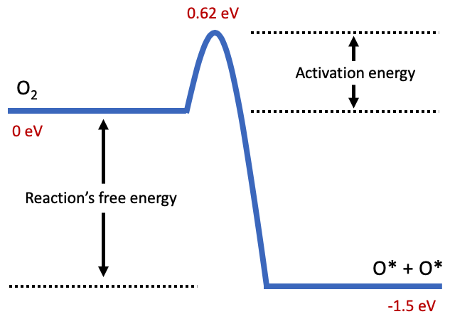
At first glance, it may be tempting to assume that all exergonic or exothermic reactions will spontaneously occur at a high rate. After all, any system will want to reduce its potential energy much like a cart let go on a hill. However, this isn’t always true. In many cases, a set of atoms will be bonded together, and be quite satisfied in their current state, such as the gas molecule in reaction (2). In terms of our analogy: The cart could have a wedge under one of its wheel to prevent it from rolling, even though it may “want to” roll downhill. In order for the oxygen atoms to bond with the catalyst, they first need to break their oxygen-oxygen bonds. Breaking this bond requires kinetic energy, and the amount of energy needed is referred to as the activation energy for the reaction, Figure 5. In our cart analogy: This is how much effort it takes to remove the wedge from under the cart’s wheel. As an extreme example, the decay of diamonds to graphite is a exergonic reaction, but due to its very high activation energy this process takes millions of years to occur!
We may think of each state in the reaction as a local minimum in the Gibbs energy with the activation energy being the height of the hills between the valleys. The primary goal of a catalyst is to reduce the activation energy, or the height of the hills between the valleys. As shown in Figure 5, the free energy between and 2 O* in (2) is -1.5eV with a platinum catalyst (eV is a unit of energy measurement that is commonly used for chemical reactions). Even though the reaction is clearly exothermic, the activation energy of reaction (2) is still 0.62 eV to break the bond. Therefore, energy (heat) needs to be added to the system in order for the reaction to occur, even though the final potential energy is lower than the initial energy. Note that in a real system, the activation energy does not act as an on/off switch. Instead, the rate of reaction gradually increases as the activation energy is approached.

The cathode’s oxygen reduction reaction (1) contains three intermediate steps. To get a complete picture of the overall reaction, we can string together Gibbs free energy plots for the three intermediate reactions to obtain Figure 6 (two steps are repeated twice to create two water molecules). The figure shows the reaction in the presence of two different catalysts, platinum and nickel. The overall reaction is exothermic using either catalyst. However, platinum has a much faster rate of reaction. Why is this? Note that the reaction’s overall free energy is independent of the catalyst used. The choice of catalyst only impacts the free energy and activation energies of the intermediate reactions. Using platinum, most of the intermediate reactions have lower activation energies. Using nickel, the oxygen atoms bind very strongly with the catalyst, resulting in a significantly lower free energy. In fact, no activation energy is needed to split in the first reaction. However due to the strong oxygen binding, the second two reactions have high activation energies, which slows the overall reaction rate.

Figure 7 shows the reaction rates of various metals as a function of the binding energy between oxygen and the catalyst. Note the reaction rate is like Goldilocks. If the binding energy is too low (strong bond) the oxygen has a hard time reacting and separating from the catalyst (nickel Ni, iron Fe). On the other hand, if the binding energy is too high (weak bond), the catalyst (silver Ag or gold Au) has a hard time attracting and holding onto oxygen atoms so that the desired reactions can take place. Platinum conveniently sits near the peak, with the “just right” bonding energy.

In the discussion above, we’ve considered the fuel cell system as if it was short-circuited, i.e., no resistance was placed on the electronic current. In practice, the circuit will have resistance, e.g., to turn on a light bulb. What effect does this have on the Gibbs free energy? Resistance in the circuit between the electrodes creates potential energy that can also be measured in volts. To find the resulting free energy given different electrode potentials, we can just subtract the potential energy per electron for each step in our reactions. As shown in Figure 8, the equilibrium potential (when the overall free energy is zero) is 1.23 eV, and the highest potential in which all reactions are exothermic is 0.78 eV. Thus the free energy of an electrochemical reaction not only helps determine its spontaneity, but also the electric potential that may be generated.
3.3.1 Reaction rate
The rate of a chemical reaction typically follows the form:
| (7) |
where is the rate of the reaction, is the “rate constant”, is the concentration of one reactant, and is the concentration of the other reactant. Thus the reaction rate is dependent on two types of quantities: the concentrations of the reactants (the inputs to the reaction) and the reaction’s rate constant. Intuitively if the concentration of the reactants is higher, the reaction rate will increase. The reaction rate constant , for which the reaction rate varies linearly, is computed using the Arrhenius equation that contains several terms:
| (8) |
where the constant encodes how frequently the reactant molecules collide and whether they have the correct orientation to react. The second term measures the probability of a collision having enough energy (velocity of the molecules) for a reaction to occur.
It is in this second term that the activation energy is needed. is divided by the temperature and the gas constant . Thus, the higher the activation energy, the higher the temperature needed to drive the reaction. If an catalyst lowers the activation energy, the reaction rate will increase for the same temperature, increasing the reaction rate.
3.3.2 Estimating reaction rates in practice
There are many factors that impact the overall rate, such as temperature, pressure, coverage (percentage of binding sites occupied), surface area of the catalyst, and the rate constant. However, there are some methods for changing the rate constant that extend beyond the relatively simple Arrhenius equation, such as changing the electrolytes used in the electrochemical cell or using promoters wang2018electrolyte; vayenas2001electrochemical (additional non-catalytic substances used to increase the reaction rate). Given all these factors it can be very difficult to directly compute the free and activation energies needed to compute the rate constant and reaction rate. However, it has been shown experimentally that the variation in the reaction rate can be approximated using only a small number of factors.
In most reactions there is a single reaction step that limits the rate of the reaction—i.e., a bottleneck reaction step. Thus only this intermediate reaction needs to be considered for determining the overall reaction rate. An intermediate reaction can be described using the change in Gibbs free energy (free energy) and the activation energy. The Gibbs free energies are computed in part (during the computation of ) based on the adsorption energy of the adsorbate on the catalyst, i.e., the change in energy of the system before and after the adsorbate bonds with the catalyst. Perhaps surprisingly, it has been shown that adsorption energies and activation energies are related by a linear function across a wide range of potential catalysts bronsted1928acid; norskov2002universality. For instance, consider reaction (2) in our oxygen reduction reaction. If a catalyst bonds more strongly to the individual oxygen atoms, it is also more likely to be able to pull apart the oxygen atoms in . The linear relation between energies results in the the ability to reasonably approximate the overall reaction rate using a linear function to predict activation energies from the adsorption energies of the intermediate adsorbates.

Depending on the catalyst, the rate limiting reaction will change. Using a technique called Sabatier Analysis sabatier1986top, the various linear relations for each rate limiting reaction can be combined by taking their minimum. The end result are plots, sometimes referred to as “volcano plots”, like those shown in Figures 7 and 9 from norskov2004origin and kulkarni2018understanding respectively. In Figure 7, the two lines signify two different rate limiting reactions: combining O and (left) and separating (right). The point indicates the transition between the two, and the optimal adsorption energy (eV) in reaction (2). A similar plot is shown in 9 for a different reaction pathway (associative vs. dissociative) for reaction (1), but in two dimensions using the energies for two intermediate adsorbates (OH and OOH). Using these approximations, the reaction rates of new catalysts can be optimized by searching for the appropriate adsorption energies per adsorbate.
It is interesting to note that for a wide range of different catalysts, they all lie roughly on a line in Figure 9. Why is this? The reason is the adsorption energies of OOH (vertical axis) and OH (horizontal axis) to a catalyst are highly correlated, since OH and OOH bond through their O atoms and not their H atoms kulkarni2018understanding. Essentially, the catalysts have a very difficult time distinguishing between these two molecules. This places limits on the types of catalyst that are likely to be found, since it is highly unlikely that a new catalyst will deviate from this trend. In order to differentiate between OH and OOH, research into more complex structures is needed kulkarni2018understanding.
Up until this point, we’ve assumed that the Gibbs, adsorption, and activation energies, which are important for determining a reaction’s spontaneity and rate, are known. How are these values computed in practice? Determining these values experimentally can be difficult, since most chemical reactions are comprised of multiple potentially unknown steps. Instead, these values are computed through numerical approximation from first principles. A popular technique for this is called Density Functional Theory (DFT) sholl2011density; parr1980density. As we explore next, DFT can produce accurate results for problems like those discussed above, but the computational cost of DFT is high. Which raises the central question of this paper: Can we train deep learning models to efficiently approximate DFT and enable the large-scale exploration of new catalysts?
3.4 Density Functional Theory
Density Functional Theory (DFT) is a popular quantum chemistry method for computing the electronic properties of an atomic structure including its energy and per-atom forces parr1980density. Here, a structure refers to a set of atoms and their 3D positions, which are input and assumed to be fixed. In our scenario, the structure includes the atoms of the adsorbate and the catalyst. Adsorbates are molecules that participate in the chemical reaction of interest, e.g., O, HO and in the oxygen reduction reaction (1).
Using the energies computed at multiple structures, we can determine the reaction’s free, adsorption, and activation energies. For instance, we can determine the adsorption energy by taking the energy difference between a structure where the adsorbate is in contact with the catalyst and a structure where the adsorbate is far away from the catalyst. A reaction’s free energy can be computed by taking the difference in energy between the final molecule and the initial molecule along with some additional corrections. Finally, if the transition state (the state corresponding to the peak in energy between two reaction steps) of a system is known, the activation energy can be computed by finding the energy difference between the reaction’s initial molecule structure and the transition structure.
DFT takes as input the positions of the structure’s atomic nuclei and computes its energy using the electron density sholl2011density. The energy of a structure, which is known as its electronic energy, refers to the potential energy, kinetic energy and other energies related to the interactions of the electrons baseden2014introduction. While we assume in our experiments that the atom nuclei are stationary (no kinetic energy), the electrons move and have both kinetic and potential energy. The energy is found using an approach that iteratively estimates the electron density of the structure until convergence. The electron density is represented using a set of spatially dependent functions, which may be either spatially localized for isolated molecules, or periodic functions for extended surfaces. This process is made possible using the Kohn-Sham equationskohn1965self. Note the term density functional theory comes from the use of functionals of the electron density, i.e., functions of the electron densities that are represented as functions.
3.4.1 Relaxations
When estimating the energy of an adsorbate interacting with a catalyst, the positions of the atoms’ nuclei are typically only roughly known. If we used DFT to calculate energies using these rough estimates, the predicted energies could be significantly overestimated, since real-world systems seek the state of lowest energy. Instead, the energy should be computed using the “relaxed” structure of the system. That is, the structure in which the atomic positions have been optimized to find the configuration with the lowest energy. The relaxation process is done iteratively using second order optimization methods. The initial atom positions are determined through heuristics based on the expected bonds. Assuming the nuclei positions are fixed, DFT is used to compute the electron densities and energy. Using derivatives of the structure’s energy, the forces on the nuclei are found and their positions updated. This process is repeated until the nuclei positions converge and the minimum energy is found. Typical relaxations require 50–400 iterations to converge. By making thermodynamic corrections (such as changes, which we don’t describe, from the term in Eqn.(5)) to the resulting energy, the structure’s Gibbs free energy can also be computed. For a more detailed explanation for how the energies and electron densities are computed, please refer to sholl2011density.
Unfortunately, there exist limitations to the use of DFT. Most importantly, it is computationally expensive and scales with respect to the number of electrons in the structure. In practice, this results in DFT relaxations taking hours–weeks per simulation using O(10–100) core CPUs on structures containing O(10–100) atoms. As a result, complete exploration of catalysts using DFT is infeasible. DFT relaxations also fail more often when the structures become large (number of atoms) and complex. It is not uncommon for relaxations to not converge, especially if the initial structure is not set properly. In practice, failure rates vary from to for the types of structures we consider in this paper. DFT would fail completely for large and more complex catalysts such as enzymes. The hope is that machine learned approximations to DFT can be both faster and potentially more stable enabling the exploration of more and larger structures.

3.4.2 Initial Structure
Before a relaxation is run, an initial structure needs to be defined. In this paper, we consider structures containing three attributes: a catalyst, an adsorbate, and a binding site. Other attributes, such as temperature and pressure, will be held constant. The catalyst is assumed to have a crystalline structure, i.e., a structure containing a repeating pattern called a “slab”. To make the DFT computations feasible, the catalyst is modeled using a single “slab” that is tiled to create the catalyst’s 2D surface. A typical slab is 6 atoms deep and 4-6 atoms across. The adsorbate is selected from the set of molecules in the reactions of interest and their intermediates.


The binding site refers to selecting the atoms that bond between the adsorbate and the catalyst. To improve the likelihood of convergence for DFT we want to select initial positions that are as close as possible to the potential binding sites. A 2D example of bonding sites is shown in Figure 10 between one, two and three atoms on the catalyst’s surface and an adsorbate with two atoms. If the adsorbate has multiple atoms, the atom of the adsorbate that bonds must also be selected. We discuss the specific set of catalysts, adsorbates and binding sites used for relaxations in Section 4.1.
3.5 Classes of Materials for Electrocatalysts
There exists an enormous space of potential materials for electrocatalysts alonso2019fundamentals. It would be overwhelming to catalog all the materials in one review. Instead, we provide some perspective on the space of materials to be considered. It is important to note that any materials dataset will necessarily contain limitations and bias.
Of the different types of materials, metal surfaces have received the greatest attention due to their reaction attributes, durability, and manufacture-ability. However, other materials are also possible, including (among many many others): surfaces with non-metallic elements, such as oxides (materials containing oxygen) seitz2016highly or nitrides (materials containing nitrogen)abghoui2017onset; metal-doped 2D materials such as graphene yang2016identification or boronitridesgrant2016selective; Perovskites (metallic oxide minerals) hwang2017perovskites that are more earth abundant and potentially less expensive; and other metal-free catalysts ma2019review. While these other material types show promise, we focus on metal surfaces in this paper given their potential for nearer term practical use and the clear applicability of DFT relaxations to their study. However, we hope the techniques developed for metal surfaces will also be useful for other material types.
Figure 11 illustrates several different types of metal structures. These include pure metals, multi-metallics (multiple unordered metal alloys), intermetallics (ordered multi-metallics), single-atom catalysts in host materials giannakakis2018single, and overlayers (surface layers of one or more metals). Alloys that contain more than three different metals are referred to as “high-entropy alloys”. Historically, the most thoroughly studied are the simplest structures containing pure metals. In contrast, the space of multi-metallics, intermetallics and overlays is significantly less well explored given the vastness of the space. For instance, choosing up to three metals from the roughly 40 possible, results in almost 10,000 combinations, and this does not even include all the possible combinations of different ratios and patterns!
Given the same underlying bulk structure, there are multiple different surfaces that may be enumerated based on which orientation you slice the material. As shown in Figure 12, the orientation of a crystalline surface or facet is typically indicated using coordinates on a unit cube. For instance, a diagonal facet is specified as (111) and results in the surface having a hexagonal pattern, whereas a (100) surface that cuts along a single dimension has a rectangular grid. In addition to flat surface types, surfaces may also contain steps, defects or other complications wang2019defect. All of these variables impact the number of different bonding sites available and how many atoms may bond to the catalyst at one time (Figure 10), which in turn impacts the overall reaction rate.
3.6 Other considerations
While we covered many of the basics for modeling catalysts, numerous improvements could be made to further improve the realism of DFT calculations. While we do not cover these items in detail, we want to make the reader aware of these topics. For those interested in a more in-depth discussion, we recommend Norskov14.
Coverage: The coverage of a catalyst refers to the percentage of surface sites that are occupied by adsorbates. As the coverage increases, the adsorbates move closer together and impact the system’s energy. For instance, the adsorption energy of the first oxygen placed on a Pt(111) surface is smaller than the adsorption energy of the 2nd, third, or fourth oxygen placed on the surfacefiorin2009microcalorimetry. Attractive and repulsive interactions between the adsorbates can also create ordered patterns of adsorbates on the surface mendez2005coadsorption.
Poisoning: Other species in the reacting mixture (even at trace levels) may poison the catalyst surface through a competitive adsorption process. Other adsorbates that do not participate directly in the reaction may adsorb strongly such that the coverage of the desired molecule and accompanying reaction rates are significantly reduced. Worse, they may bind so strongly that they never leave, thereby rendering the catalyst inert. These molecules occupy the potential bonding sites of the desired adsorbates, and essentially “poison” the catalyst. A common example is the poisoning of noble metal catalysts by lead, or poisoning of platinum catalysts by trace carbon monoxide.
Electrolytes: Most electrochemical reactions occur in the presence of an aqueous or solid electrolyte to conduct charged particles to the surface, e.g. they are submerged in water/electrolyte solution to increase the conductivity of the system and therefore improve reactivity. The precise solvent (water or otherwise) can affect adsorption energies, most notably for adsorbates that can form hydrogen bonds with the water layer. Further, electrolytes such as KOH or NaCl can be added to the water to further improve reaction performance. They do this by interacting with the adsorbates and catalyst to stabilize the transition states of particular reaction intermediates, thereby reducing the activation energy and accelerating the reaction rate. Sometimes these effects are modeled by making simple corrections to the energies found without electrolytes, but ideally the electrolytes would be modeled directly. There are major scientific challenges remaining in our understanding of these processes.
Catalyst Dynamics: In the real world, the atoms in the system are constantly moving. The more heat that is applied to a system, the faster the atoms move. Molecular dynamics models the movement of these atoms by integrating the standard equations of motion (). Since the atoms may be fast moving and visiting a wider range of potential surfaces and sites, modeling these systems can be more challenging than the relaxations (with zero kinetic energy) we describe in this paper. The real catalyst may re-arrange under reaction conditions or form an ensemble of different states that all contribute to the final activity. Modeling these processes requires molecular dynamics simulations, but accessing experimentally-relevant timescales (nanoseconds) requires approximately 106 force calls at the atomic (femtosecond) timescale and are thus vastly more expensive than standard DFT relaxations. Approaches to exploring this problem use both standard DFT rapaport2004art and learned models schutt2018schnet; li2015molecular; behler2016perspective; chmiela2017machine.

4 ML for Electrocatalysis
In this section, we begin by providing a short overview of the problem, followed by the dataset, tasks, and approaches for addressing it. For those interested in a more detailed discussion of the problem, please refer to Sections 2 and 3.
As intermittent renewable energy sources (solar and wind) become more prevalent, the storage of their energy from times of peak generation to peak demand will increase in importance. The use of renewable energy to generate other fuels that are easily stored provides a potential solution to this problem that can scale to nation-sized grids. For instance, renewable energy can be used to split water into hydrogen and oxygen gas. The stored hydrogen is then used to generate electricity at a later time using fuel cells. Currently, a major limiting factor is finding efficient, durable and cheap catalysts for driving the electrochemical reactions involved in this process.
A catalyst increases the rate of a chemical reaction while not being consumed in the process. During a chemical reaction the molecules involved in the reaction, called adsorbates, interact with the catalyst’s surface. The change in energy when the adsorbate comes in contact with the catalyst, called the adsorption energy, is the key factor is determining the overall reaction’s rate (Section 3.3.2). The adsorption energy must be neither too high (the catalyst holds on to the adsorbates too strongly) nor too low (the adsorbates float away from the catalyst). If the reaction’s rate is increased, the overall efficiency of the system increases and costs decrease. The challenge is finding catalysts that not only increase the reaction’s rate, but are also cheap to produce, e.g., are not made of expensive metals such as platinum.
The adsorption energy is computed by first finding the positions of the atoms when the adsorbate comes in contact with the catalyst’s surface. In the real-world, the atoms seek a configuration that reduces the overall energy of the system. The set of 3D atom positions at a local energy minimum is referred to as a “relaxed structure” and the corresponding system energy as the “relaxed energy”.
How is a relaxed structure estimated computationally? An iterative process is used that first roughly places the adsorbate near the catalyst to create an initial structure. For any given pair of adsorbate and catalyst, numerous initial structures may exist based on the binding site chosen, Figure 10. The selection of an adsorbate’s binding site and its initial positioning relative to it is heuristically determined. Next, the per-atom forces are computed, from which atom positions are updated using BFGS head1985broyden or conjugate gradient techniques. The forces are re-estimated and atom positions updated until the forces converge to zero at which point a local energy minimum has been found. Typically, hundreds of iterations are necessary to converge to a relaxed structure. While this process seems simple, the computation of the atom forces is highly complex and computationally very expensive.
Atom forces and a structure’s energy are computed using Density Functional Theory (DFT) sholl2011density; parr1980density, which is computationally expensive and can take hours to calculate for a single structure. How can we scale the simulation of new catalysts from hundreds or thousands to billions? A promising alternative to expensive DFT calculations is to train efficient machine learning models to approximate DFT. The model takes as input the set of atoms, including their atomic numbers and 3D positions, and computes the per-atom forces. Similar to DFT, the force estimates may be used to find relaxed structures. To eliminate the need for DFT entirely, models may be trained to also estimate a structure’s energy.
Machine learning models that employ deep learning require large datasets for training. We begin by describing the Open Catalyst Dataset (OC20) created for this purpose; followed by deep learning approaches that have been proposed for estimating DFT and metrics for evaluating the models. We strive to release all data and code in accordance with FAIR (Findable, Accessible, Interoperable, Reusable) principles wilkinson2016fair.

4.1 Open Catalyst Dataset (OC20)
An ideal dataset would enable the exploration of new techniques for estimating DFT calculations while also helping the catalysis community explore new materials and gain a deeper understanding of the physics underlying catalysts—overall accelerating progress towards discovering better alternatives to commonly used catalysts. This requires both a large (for learning) and diverse (for generalization and exploring new materials) dataset. For the dataset, priority is given to catalysts with relatively near-term practical potential, and adsorbates relevant to the reactions used in renewable energy storage. Specifically, we explore metallic surfaces, which are currently the most popular catalysts in use due to their durability, ease of manufacture, and efficiency.
Our OC20 dataset OCD1M20 contains over a million relaxations of randomly selected catalysts and adsorbates from a set of potential candidates. On average each relaxation contains approximately 200 structures in its trajectory from the initial structure to the relaxed structure, which results in over 130+ million structures for training with the rest used for validation and testing. Example adsorbate and catalyst pairs are shown in Figure13, and example initial and relaxed structures in Figure 14. All calculations are performed using VASP (Vienna Ab initio Simulation Package) kresse1993ab; kresse1994ab; kresse1996efficiency; kresse1996efficient, which is a popular package for performing the types of DFT calculations used in this paper.
A detailed description of the OC20 dataset and its various design choices are provided in OCD1M20. In this paper, we cover the necessary details to build and evaluate models with the dataset. We begin by describing the various tasks, followed by the inputs and data splits.

4.1.1 Tasks and Evaluation Metrics
We identify three tasks based on their practical applicability to cataylst design. Since structure relaxations are the primary tool for determining a catalyst’s utility, we focus on modeling this process and its outputs. As shown in Table , task outputs include per atom forces and positions, and the energy of a structure. The relationship of each of our tasks is shown in Figure 15. Per task evaluations may be performed on the validation set using the supplied code and ground truth data. Test set evaluations may be performed by uploading results to the Open Catalyst Project leaderboard. Our three tasks are as follows:
S2EF - Structure to Energy and Forces
task is given a structure as input, predict the per-atom forces and structure’s energy as output. This task mirrors the computationally expensive DFT calculation. An efficient approximation to DFT would be beneficial to numerous tasks, including relaxations. Evaluation is performed using the Mean Average Error (MAE) between the computed forces and energies and those computed using DFT. In addition, a third evaluation metric determines the percentage of predictions with Energy and Forces within a Threshold (EFwT) of the ground truth. By using tight thresholds, the EFwT metric provides an estimate for how often the predictions would be practically useful.
IS2RS - Initial Structure to Relaxed Structure
task estimates the relaxed structure given the initial structure as input. This task may be performed iteratively using S2EF calculations, similar to how traditional relaxations are computed, Figure 15(b). We refer to these calculations as ML relaxations, since ML models are used to compute the relaxations. An alternative is to compute the final 3D positions of the atoms directly from their initial structure, Figure 15(c).
Evaluations are performed using two techniques. The first measures the 3D positional differences between the ML computed relaxed structure and the structure computed using a traditional DFT relaxation. Since small changes in position can lead to significant changes in forces and energies, distance metrics by themselves are insufficient for determining whether a true relaxed structure is found. The second metric uses a single DFT calculation to determine the forces on the proposed relaxed structure. If a true local minimum was found, the forces as computed by DFT should be close to zero. The final metrics compute the percentage of ML relaxed structures with maximum force magnitudes below a threshold. Since DFT calculations are computationally expensive, IS2RS force metrics reported on the Open Catalyst Project test server are only evaluated on a subset of the test splits. The 3D distance metric is computed using the entire test set.

IS2RE - Initial Structure to Relaxed Energy
task computes the relaxed structure’s energy from the initial structure. The relaxed energy is used to compute the adsorption energy, i.e., the change in energy when the adsorbate comes in contact with the catalyst. As discussed in Section 3.3.2, the adsorption energy is informative in predicting the activation energies and ultimately the rate of the reaction in the presence of the catalyst. While we focus on the system’s energy, other system properties may also be estimated. For instance, the popular QM9 dataset ramakrishnan2014quantum containing small organic molecules, estimates 13 energetic, electronic, and thermodynamic properties.
Similar to IS2RS, IS2RE may be accomplished using two approaches: The first iteratively estimates the relaxed structure and its corresponding energy using S2EF, Figure 15(b). The second, directly computes the relaxed energy from the initial structure, Figure 15(d). Using the second approach, IS2RE does not require the estimation of the relaxed structure. Evaluation is performed using MAE between the estimated relaxed energies and those found using DFT relaxations, as well as, the percentage of energy estimates within a tight threshold of the ground truth.
4.1.2 Inputs
The inputs to the OC20 tasks include the atoms, catalyst and adsorbate information. We discuss each in turn.
Atoms
A structure contains catalyst and adsorbate atom information at a specific instance in time. This includes the atoms’ 3D positions, along with various per-atom and per-pair (of atoms) proprieties, as shown in Table . Per-atom information includes the atom’s group and period number, electronegativity, covalent radius, etc. The per-pair properties include the distance between the atoms and their predicted bond type.
Catalyst
Along with the atom information described above, additional information is provided for the catalyst. Each catalyst contains 1 to 3 types of elements, with , , and of the OC20 catalysts being unary, binary, and ternary materials respectively. Stable catalyst materials were randomly selected from those contained in the Materials Project jain2013commentary. A catalyst is modeled as an infinite 3D surface with a repeating 2D crystalline structure in the x and y dimensions. The adsorbate sits on top of the catalyst in the z dimension with the catalyst extending infinitely below the adsorbate. As input, only a single crystalline structure, known as a slab, is given that can be replicated or tiled in cells to create the full 3D surface. A 2D illustration of this process is shown in Figure 16. When computing atom interactions, the set of neighboring atoms needs to be determined. Since the slab is repeated in each cell, the atoms on the far right of a slab (atom in Fig. 16) may be neighbors to those on the far right of the next cell over (atom and in Fig. 16), and similarly for all other x and y directions. The atom positions can be transformed from one cell to the next using a matrix :
| (9) |
where is the 3D cell indicator vector, e.g., or , is the atom’s position in the slab, and is the position of the atom in the indicated cell.
Instead of tiling the slab in the z direction, it is assumed that only atoms near the surface of the catalyst will move. Each atom in the structure is given a variable that indicates whether it is assumed to be fixed or is free to move. All atoms in the adsorbate are free, and typically the top two layers of atoms in the catalyst are free and the rest fixed (dark and light blue atoms in Fig. 16). Note that DFT computes the forces assuming that the slab is not tiled in the z direction, so the forces of the bottom atom layers in the catalyst may be very large as they try to expand. Only free atoms are used when evaluating computed positions and forces. The forces of the fixed atoms may be used for training if desired.
| Reaction | Name | Purpose |