Neural Network Architectures for Location Estimation in the Internet of Things
Abstract
Artificial Intelligence (AI) solutions for wireless location estimation are likely to prevail in many real-world scenarios. In this work, we demonstrate for the first time how the Cramer-Rao upper bound on localization accuracy can facilitate efficient neural-network solutions for wireless location estimation. In particular, we demonstrate how the number of neurons for the network can be intelligently chosen, leading to AI location solutions that are not time-consuming to run and less likely to be plagued by over-fitting. Experimental verification of our approach is provided. Our new algorithms are directly applicable to location estimates in many scenarios including the Internet of Things, and vehicular networks where vehicular GPS coordinates are unreliable or need verifying. Our work represents the first successful AI solution for a communication problem whose neural-network design is based on fundamental information-theoretic constructs. We anticipate our approach will be useful for a wide range of communication problems beyond location estimation.
I Introduction
Several traditional localization algorithms have been developed to estimate the location of a vehicle in the past, e.g., [1, 2, 3, 4, 5]. The practical limitations with these algorithms may range from limited functionalities to a complete failure as the surrounding environment changes. Therefore, we need localization algorithms that are practically deployable, smart enough to adapt to the environmental changes, and that are realistic.
To address the challenges that traditional localization algorithms face, researchers in recent times have incorporated numerous neural-network and machine-learning algorithms for positioning users/devices [6, 7]. While neural-networks have been able to address the shallow learning capabilities of the classic machine-learning algorithms, a key question about neural-networks, that is yet to be answered, is how to design their internal architecture, i.e., the number of chosen hidden layers, the choice of activation function in the hidden layer(s), and the number of neurons in each hidden layer. While the research community follows hyperparameters search mechanisms to finalize the architecture for neural-network frameworks at large [8], numerous guidelines have also been provided in the recent literature to formulate an optimal neural-network architecture [9, 10]. However, to-date there has been no concrete solution on how to pre-determine a neural-network architecture for a given problem.
In this work, we develop a feedforward neural-network framework for location estimation and formulate an insight into its architecture. We use received signal strength (RSS) of the vehicles’ transmitted signals measured at multiple static road side units (RSUs). Through analysis based on the Cramer-Rao upper Bound (CRB) on the location accuracy of a vehicle, we identify an architecture for a neural-network-based location estimation framework (NNLEF). Detailed numerical analysis confirms our analysis.
Although the concepts discussed here are in the context of vehicular adhoc networks (VANETs), they are widely applicable to a range of location-centric applications within the domain of internet of things. Beyond the contribution stated above we summarize our additional contributions thus:
- 1.
We derive a value for the number of neurons needed in the hidden layer.
- 2.
Through simulated data, we show how the NNLEF (with the adopted architecture) outperforms when compared to other NNLEFs (that follow random architectures).
- 3.
We further show how the NNLEF (with the adopted architecture) performs more efficiently when compared to a traditional RSS-based algorithm.
- 4.
Finally, we experimentally validate our recommended architecture.
The remainder of this paper is organized as follows. Section II details the system model and the derivation of the CRB on location accuracy. Section III presents the NNLEF. Section IV provides numerical results based on simulated and experimental data, and Section V concludes this paper.
II System Model and RSS Location Estimation
We consider the following system model in our work:
- 1.
The true location of a random vehicle (which is unknown to the framework) is denoted by .
- 2.
The framework has number of RSUs with publicly known locations. The true location of the i-th RSU is where .
- 3.
All the RSUs are in the transmission range of the randomly located vehicle and independently measure RSS (all RSS in dBm) of the transmitted signal (from the random vehicle) every second. We adopt a log-normal shadowing model for the RSS observations. The measured RSS at the i-th RSU, i.e., , is given as
where is the transmit power of the vehicle and (the path loss at a distance ) is given by
where is the reference path loss at a reference distance , is the path loss exponent, is the vehicle-RSUi distance given by , and is a zero mean normal random variable with variance representing the shadowing noise. The RSS measurements made by the RSUs are independent of each other. They collectively form an RSS vector given by .
- 4.
We choose one of the RSUs as the processing center (PC). The PC accumulates its RSS measurements with the regularly collected RSS measurements from all surrounding RSUs. The PC further processes these measurements to estimate the location of the random vehicle. The estimated location of the vehicle is denoted by .
II-A Cramer-Rao Upper Bound Derivation
We now derive the CRB on the location accuracy of a vehicle. For a random transmitting vehicle, whose location is unknown, and whose RSS is measured at RSUs, the distribution of the RSS takes the form (with few constant elements ignored)
The covariance matrix (related to the position) can be written as the inverse of the Fisher information matrix, , i.e., . The elements of are given by
where
where denotes the expectation operation. The expressions in brackets are given as,
where .
We consider and extract the final expressions for the elements of as,
The final expression for CRB can be written as, . Here and are the diagonal elements of , and equals the standard deviation of the CRB.

To draw the ellipses representing the CRB on location accuracy in terms of confidence levels (CLs), the rotation matrix is required, and is given by
where , while and are the eigenvectors of . The range of is in between and . The probability of a vehicle’s location (returned by a positioning system) lying within a CL ellipse is given below [11]
where is a constant that sets the scaling of the confidence ellipse.
Using our derivation, we draw in Fig. 1 ellipses with different CLs for 2 sample test points. The locations of the RSUs are (50m, 50m), (50m, 200m), (125m, 125m), (200m, 50m), and (200m, 200m). The value of is fixed at 5dB, and the path loss exponent equals 3.
III Neural-network based Location Estimation
This section highlights the adopted NNLEF’s performance in relation to estimating a vehicle’s location. A feedforward neural-network forms the basis of this framework. This framework utilizes the measured RSS (influenced by the shadowing noise) at multiple RSUs. A feedforward network is a special type of neural-network that is known to manipulate and learn from the physical layer properties of the vehicles’ transmitted signals [12, 13, 14]. Neural-network frameworks with a single, or multiple hidden layers, have the capability to converge to a continuous target function. However, a single hidden layer neural-network framework has a more flexible learning rate and converges faster to the target function when compared to a multiple hidden layer neural-network framework [15]. The architecture for the neural-network framework in this work is thus limited to a single hidden layer.
We next focus on developing an intuition into the performance of the NNLEF with changing activation functions and with a varying number of neurons in the hidden layer. It is evident from the expressions of a logistic sigmoid activation function, i.e., , and a tangent sigmoid activation function, i.e., , that the gradient for both these activation functions at absolute high values is approximately zero. With complex data at the input, this phenomenon can minimize learning for the NNLEF. On the other hand, a steady gradient for the ReLu activation function, , keeps the framework’s learning consistent in the region where and there is a possibility of faster learning for the NNLEF [16, 17]. We have investigated and found that different transfer functions in the hidden layer of the NNLEF produce comparable results. In order to accommodate for future complex channel environments we take into account ReLu as the choice of transfer function for the hidden layer of the NNLEF.

The input to the NNLEF comprise r. The number of outputs is set to 2 (the location coordinates). A schematic of the NNLEF in this work is shown in Fig. 2. The number of neurons in the hidden layer, , is our focal point in this study. The text in the following paragraphs will provide an insight into a recommendation for . This recommendation for will allow for a promising performance of the NNLEF. Each neuron in the hidden layer of the NNLEF partially contributes towards the performance of the NNLEF. A very small is likely not sufficient to extract the hidden features/patterns in the input data. A reasonable is therefore required for the NNLEF to perform efficiently. Increasing is expected to produce good results (Figs. 3 and 5 highlights this phenomenon) but is not, in general, advised as this only adds to the framework’s overhead. That is, increasing can improve the NNLEF’s performance marginally, but at the cost of an unnecessary increase in the NNLEF’s overhead (e.g., the number of parameters, computational time, and memory resources). Additionally, with a very high , the NNLEF can lead to an over-fitting problem especially in conjunction when too much training data is supplied under one specific channel condition.
Two critical questions are faced in the design of any neural network algorithm. One is: How much training of the algorithm should occur? A second is: What should the architecture be (how many neurons)? Consider a channel that is perfectly described by some model, and this is used for training purposes. If we were to train a neural network under this model with unconstrained training samples (RSS values and all location information) and unconstrained (the number of neurons to be placed in the hidden layer) we would be identifying perfectly, in effect, the function that describes the models distance vs. RSS relation. Given this perfect channel identification any use of that network to determine an unknown location from noisy RSS values should achieve a location error at the CRB11 1 However, in real-world scenarios we could expect the location accuracy of such a network be substantially less than the CRB. The reason for this is that, in general, the real-world channel will never be exactly the training model..
In estimating , we would like to ensure that any loss in the network performance (distance accuracy) introduced by constraining that number is not too large. As we now show, the Universal Approximation Theorem (UAT) [18] can allow insight into that. Loosely speaking, the UAT states that there always exists a neural network that can approximate any input function, , with any output function, , to any arbitrary accuracy , i.e. . In our case RSS and maps to the distance, , between transmitter and receiver.
To make progress let us consider a single hidden layer neural network with transfer functions of the sigmoid form (our result will be independent of this choice). A neuron is modelled by , where . It is straightforward to show that values of and can be chosen to ‘force’ the transfer function into a step form where the step occurs at . Further, by using transfer functions ( neurons) connected in a single layer network, it is straightforward to show that a series of rectangles can be formed at the output [19]. That is, you can create a network that can model any input function as an output function consisting of a series of rectangles. If we simplify this further and make all the rectangles of equal width, we can easily determine such that , where now represents the standard deviation in the distance difference between the two functions. The CRB on the distance estimate for log-normal shadowing is . Therefore, a good estimate of our required would be one that ensures . Carrying out the calculation detailed above, taking a typical distance scale of order 100m we find the following: Adopting and we find that ; adopting and we find we find that ; and adopting and we find we find that ; This indicates in the range of 7-12 would be useful for the type of channels we investigate here.
IV Numerical Results
IV-A Analysis Using Simulated Data
We now present our numerical results by taking into account simulated data. The focus area is of size 200m200m. 5 RSUs are installed at (0m, 0m), (0m, 200m), (100m, 100m), (200m, 0m), and (200m, 200m). The focus area resembles a cross section of an expressway. The horizontal and vertical axes are partitioned into equidistant divisions. The RSUs measure RSS from the cross section of the divisions on both the axes at a frequency of 1Hz. The RSS measurements are under the influence of random shadowing noise. To mimic reality and to accommodate for the unique location of each RSU, this noise element is extracted from a random Gaussian distribution with a fixed . This means that at any given instant, the RSS measurements from a cross section of the divisions on all the RSUs will have unique and independent shadowing noise elements included in them. A value of 5dB is taken into account for . The path loss exponent is set to 3. After the RSS measurement campaign, the RSS database is randomized and further divided into two sets; a test set (with nearly 10% of the database samples), and a training set (with the remaining database samples). The training set has the horizontal and vertical coordinates for the cross section of the divisions, while the test set has no such information included.

In Fig. 3 we study the performance of the NNLEFs with changing . For uniformity, we use a ReLu activation function in the hidden layer of all the NNLEFs. Moreover, all the other neural-network training parameters are kept the same. We train all the NNLEFs with the same training set data. Once the training concludes, we subject the NNLEFs to estimate locations for the vehicles in the test set. To analyze the performance, we draw confidence ellipses with different CLs and plot the estimated locations by each NNLEF. To determine whether an NNLEF’s estimated location is within or outside a particular confidence ellipse, we use the equation below
where is the center of the ellipse, is the length of the semi-major axis, and is the length of the semi-minor axis for a particular confidence ellipse. In Fig. 3 we plot the percentage of the NNLEFs’ estimated test locations in each confidence ellipse (on the y-axis) against (on the x-axis). The changing on x-axis corresponds to different NNLEFs. We apply a polynomial fitting of order 7 for curve smoothing. The green, blue, and black curves represent the percentage of estimated locations by the NNLEFs in ellipses with CLs 39%, 66%, and 95%, respectively. The dashed colored lines represent the CRBs on location accuracy for the corresponding confidence ellipses (derived in section II-A). From the figure, we observe that the performance for the NNLEF becomes approximately consistent when 8. We do see negligible performance improvement for a few random NNLEFs with in the higher range. These NNELFs are not recommended as they will increase the number of training parameters and computational costs by many folds which do not justify the minimal performance improvement. For example, the number of training parameters for the NNLEF with 8, 30, 40, and 50 neurons in the hidden layer is 66, 242, 322, and 402, respectively.
Next, we compare the performance for the NNLEF (with in the recommended range, i.e., 8) with a state-of-the-art RSS based algorithm. The RSS based algorithm minimizes the root mean square error between the measured RSS values in the test and training set to estimate a vehicle’s location, i.e.,
where , and are the testing and training set RSS vectors, respectively, and represents the total number of samples in the training set. In Fig. 4 we plot the percentage of the estimated test locations in each confidence ellipse.

In order to further validate the performance for the NNLEF with the derived architecture, i.e., 8, in comparison to other NNLEFs with random architectures, i.e., with equal to 3, 20, 30, 40, and 50, we use a different performance metric as in [7], i.e., mean square error (MSE), which is defined as MSE = . Using the same parameter settings as used in Fig. 3, we plot the MSE for all the NNLEFs in Fig. 5. The x-axis indicates the MSE bin spacing in tens of meters, while the y-axis shows the number of samples in each MSE bin. The solid arrow pointing at the x-axis is the 1 CRB in meters. We see an equivalent performance for all the frameworks. This highlights the fact that a high does not always relate to the NNLEF’s performance improvement.

IV-B Analysis Using Real-world Data
We now present numerical results by taking into account real-world RSS measurements. These measurements have a multipath factor (from the ground) and noise elements in them. The RSS measurements from random vehicles were collected in a 150 X 150 square meters area by 3 RSUs (installed at (0m, 0m), (-25.5m, 47.6m), and (-8.6m, -46.9m)). 3 devices were used to mimic 3 RSUs. Each device independently measured RSS from the random vehicles at a frequency of 1 RSS measurement per second. Slowly moving Wi-Fi modems (802.11g) with a single antenna (at the same height as RSUs antennas), and a transmission frequency of 2.437 MHz were used to represent slow moving vehicles. These vehicles, equipped with GPS units, reported their GPS locations to the RSUs every second. The RSS measurements at the individual RSUs and the GPS locations of the vehicles were combined utilizing the time stamps (available with both the RSS measurements and the vehicles’ GPS locations).
At the end of the measurement campaign, the RSS measurement data was thoroughly randomized and divided into a training set (with 85% of the measurement data) and a test set (of the remaining 15% measurement data). The training set had the location information of the vehicles while the test set had no such information included. All the NNLEFs (with different ) were trained using the training set. The trained NNLEFs’ were then used to estimate the locations of the vehicles in the test set. In Fig. 6, we plot the percentage of the estimated test set locations for NNLEFs with changing in the ellipse with 95% CL (with polynomial fitting applied). From the figure we observe that performance for the NNLEFs becomes asymptotic once exceeds 8. This validates our earlier claim that a higher may not add much to the performance of the NNLEF, rather it would result in an increase in the computational overheads.

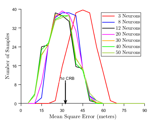
We, next compare the performance of an NNLEF with = 8 and 12 (in line with our recommended range for ) and other NNLEFs with random using MSE metric in Fig. 7. We notice that NNLEF with too low a , i.e., 3, performs poorly. We also see nearly equivalent performance for the NNLEF (with = 8 and 12 neurons) when compared to the other NNLEFs (with high ). Here, we observe that NNLEF with = 12 is performing slightly better than NNLEF with = 8.
V Conclusion
In this work we have shown, for the first time, how information-theoretic constructs can be used to decide the number of hidden-layer neurons within neural-network architectures for wireless location estimation. Our analysis is confirmed with both simulated data and real-world-data. Our work provides insight into pragmatic architecture design for a wide range of neural-network frameworks beyond location estimation.
VI Acknowledgment
The authors acknowledge support by the University of New South Wales, Australia, and Macquarie University, Australia. Ullah Ihsan acknowledges financial support from the Australian Government through its Research Training Program.
References
- [1] E. Lee, S. Yang, S. Oh, and M. Gerla, “RF-GPS: RFID assisted localization in VANETs,” in Proceedings of the IEEE Conference on Mobile Adhoc and Sensor Systems, Macau, China, Oct. 2009, pp. 621–626.
- [2] K. Golestan, S. Seifzadeh, M. Kamel, F. Karray, and F. Sattar, “Vehicle localization in VANETs using data fusion and V2V communication,” in Proceedings of the ACM International Symposium on Design and Analysis of Intelligent Vehicular Networks and Applications, Paphos, Cyprus, Oct. 2012, pp. 123–130.
- [3] N. Alam, A. Balaei, and A. Dempster, “Relative positioning enhancement in VANETs: A tight integration approach,” IEEE Transactions on Intelligent Transportation Systems, vol. 14, no. 1, pp. 47–55, Jul. 2012.
- [4] G. Hoang, B. Denis, J. Härri, and D. Slock, “Cooperative localization in GNSS-aided VANETs with accurate IR-UWB range measurements,” in Proceedings of the IEEE Workshop on Positioning, Navigation and Communications, Bremen, Germany, Oct. 2016, pp. 1–6.
- [5] S. Cruz, T. Abrudan, Z. Xiao, N. Trigoni, and J. Barros, “Neighbor-aided localization in vehicular networks,” IEEE Transactions on Intelligent Transportation Systems, vol. 18, no. 10, pp. 2693–2702, Feb. 2017.
- [6] H. Chen, Y. Zhang, W. Li, X. Tao, and P. Zhang, “ConFi: Convolutional neural networks based indoor Wi-Fi localization using channel state information,” IEEE Access, vol. 5, pp. 18 066–18 074, Sep. 2017.
- [7] A. Kumar and V. Jain, “Feed forward neural network-based sensor node localization in Internet of Things,” in Progress in Computing, Analytics and Networking. Springer, 2018, pp. 795–804.
- [8] J. Bergstra and Y. Bengio, “Random search for hyper-parameter optimization,” Journal of Machine Learning Research, vol. 13, no. 10, pp. 281–305, Feb. 2012.
- [9] I. Goodfellow, Y. Bengio, and A. Courville, Deep Learning. MIT Press, 2016, http://www.deeplearningbook.org.
- [10] J. Heaton, Artificial Intelligence for Humans, Volume 3: Deep Learning and Neural Networks. Heaton Research, Inc., Dec. 2015.
- [11] R. Malaney, “Securing Wi-Fi networks with position verification: extended version,” International Journal of Security and Networks, vol. 2, no. 1-2, pp. 27–36, 2007.
- [12] U. Ihsan, R. Malaney, and S. Yan, “Machine learning and location verification in vehicular networks,” in Proceedings of the 8th IEEE/CIC International Conference on Communications in China (ICCC2019), Changchun, China, Aug. 2019, pp. 91–95.
- [13] U. Ihsan, S. Yan, and R. Malaney, “Location verification for emerging wireless vehicular networks,” IEEE Internet of Things Journal, vol. 6, no. 6, pp. 10 261–10 272, Aug. 2019.
- [14] U. Ihsan et al., “Artificial intelligence and location verification in vehicular networks,” in Proceedings of the IEEE Globecom, Waikoloa, HI, USA, Dec. 2019, pp. 1–6.
- [15] T. Nakama, “Comparisons of single-and multiple-hidden-layer neural networks,” in Proceedings of the International Symposium on Neural Networks, Guilin, China, Jun. 2011, pp. 270–279.
- [16] A. Krizhevsky, I. Sutskever, and G. Hinton, “Imagenet classification with deep convolutional neural networks,” in Proceedings of the Neural Information Processing Systems, Lake Tahoe, NV, USA, Jan. 2012, pp. 1097–1105.
- [17] C. Bircanoğlu and N. Arıca, “A comparison of activation functions in artificial neural networks,” in Proceedings of the IEEE Signal Processing and Communications Applications Conference (SIU), Izmir, Turkey, May, 2018, pp. 1–4.
- [18] K. Hornik, M. Stinchcombe, and H. White, “Multilayer feedforward networks are universal approximators.” Neural networks, vol. 2, no. 5, pp. 359–366, Mar. 1989.
- [19] M. Nielson, in Neural Networks and Deep Learning. Determination Press, 2015.