Visibility Optimization for Surveillance-Evasion Games

Louis Ly Yen-Hsi Richard Tsai Affiliation: louisly@utexas.edu, ytsai@math.utexas.edu Affiliation: [3em] Oden Institute for Computational Engineering and Sciences Affiliation: The University of Texas at Austin

Abstract

We consider surveillance-evasion differential games, where a pursuer must try to constantly maintain visibility of a moving evader. The pursuer loses as soon as the evader becomes occluded. Optimal controls for game can be formulated as a Hamilton-Jacobi-Isaac equation. We use an upwind scheme to compute the feedback value function, corresponding to the end-game time of the differential game. Although the value function enables optimal controls, it is prohibitively expensive to compute, even for a single pursuer and single evader on a small grid. We consider a discrete variant of the surveillance-game. We propose two locally optimal strategies based on the static value function for the surveillance-evasion game with multiple pursuers and evaders. We show that Monte Carlo tree search and self-play reinforcement learning can train a deep neural network to generate reasonable strategies for on-line game play. Given enough computational resources and offline training time, the proposed model can continue to improve its policies and efficiently scale to higher resolutions.

1 Introduction

We consider a multiplayer surveillance-evasion game consisting of two teams, the pursuers and the evaders. The pursuers must maintain line-of-sight visibility of the evaders for as long as possible as they move through an environment with obstacles. Meanwhile, the evaders aim to hide from the pursuers as soon as possible. The game ends when the pursuers lose sight of the evaders. We assume all players have perfect knowledge of the obstacles and the game is closed-loop – each player employs a feedback strategy, reacting dynamically to the positions of all other players.

In section 3, we consider the game in the context of Hamilton-Jacobi-Isaacs (HJI) equations. We propose a scheme to compute the value function, which, informally, describes how ”good” it is for each player to be in a specific state. Then each player can pick the strategy that optimizes the value function locally. Due to the principal of optimality, local optimization with respect to the value function is globally optimal. This is because the value function encodes information from all possible trajectories. As a result, the value function is also very expensive to compute.

Section 4 discusses locally-optimal policies and section 5 presents search-based methods to learn policies for the multiplayer version of the game.

1.1 Related works

The surveillance-evasion game is related to a popular class of games called pursuit-evasion [15, 16], where the objective is for the pursuer to physically capture the evader. Classical problems take place in obstacle-free space with constraints on the players’ motion. Variants include the lion and man [18, 30], where both players have the same maneuverability, and the homicidal chauffeur [23], where one player drives a vehicle, which is faster, but has constrained mobility. Lewin et. al. [22] considered a game in an obstacle-free space, where the pursuer must keep the evader within a detection circle.

Bardi et. al. [2] proposed a semi-Lagrangian scheme for approximating the value function of the pursuit-evasion game as viscosity solution to the Hamilton-Jacobi-Isaacs equation, in a bounded domain with no obstacles. In general, these methods are very expensive, with complexity $\mathcal{O}(m^{kd})$ where $k$ is the number of players and $d$ is the dimension. This is because the value function, once computed, can provide the optimal controls for all possible player positions. A class of methods try to deal with the curse of dimensionality by solving for the solutions of Hamilton-Jacobi equations at individual points in space and time. These methods are causality-free; the solution at one point does not depend on solutions at other points, making them conveniently parallelizable. They are efficient, since one only solves for the value function locally, where it is needed, rather than globally. Chow et. al. [8, 9, 10] use the Hopf-Lax formula to efficiently solve Hamilton-Jacobi equations for a class of Hamiltonians. Sparse grid characteristics, due to Kang et. al. [17], is another causality-free method which finds the solution by solving a boundary value problem for each point. Unfortunately, these methods do not apply to domains with obstacles since they cannot handle boundary conditions.

The visibility-based pursuit-evasion game, introduced by Suzuki. et. al [34], is a version where the pursuer(s) must compute the shortest path to find all hidden evaders in a cluttered environment, or report it is not possible. The number of evaders is unknown and their speed is unbounded. Guibas et. al. [14] proposed a graph-based method for polygonal environments. Other settings include multiple pursuers [33], bounded speeds [37], unknown, piecewise-smooth planar environments [28], and simply-connected two-dimensional curved environments [21].

The surveillance-evasion game has been studied previously in the literature. LaValle et. al. [20] use dynamic programming to compute optimal trajectories for the pursuer, assuming a known evader trajectory. For the case of an unpredictable evader, they suggest a local heuristic: maximize the probably of visibility of the evader at the next time step. They also mention, but do not implement, an idea to locally maximize the evader’s time to occlusion.

Bhattacharya et. al. [4, 6] used geometric arguments to partition the environment into several regions based on the outcome of the game. In [5, 44], they use geometry and optimal control to compute optimal trajectories for a single pursuer and single evader near the corners of a polygon. The controls are then extended to the whole domain containing polygonal obstacles by partitioning based on the corners [45], for the finite-horizon tracking problem [43], and for multiple players by allocating a pursuer for each evader via the Hungrarian matching algorithm [42].

Takei et. al. [36] proposed an efficient algorithm for computing the static value function corresponding to the open loop game, where each player moves according to a fixed strategy determined at initial time. Their open loop game is conservative towards the pursuer, since the evader can optimally counter any of the pursuer’s strategies. As a consequence, the game is guaranteed to end in finite time, as long as the domain is not star-shaped. In contrast, a closed loop game allows players to react dynamically to each other’s actions.

In [7, 13, 35], the authors propose optimal paths for an evader to reach a target destination, while minimizing exposure to an observer. In [13], the observer is stationary. In [7], the observer moves according to a fixed trajectory. In [35], the evader can tolerate brief moments of exposure so long as the consecutive exposure time does not exceed a given threshold. In all three cases, the observer’s controls are restricted to choosing from a known distribution of trajectories; they are not allowed to move freely.

Bharadwaj et. al. [3] use reactive synthesis to determine the pursuer’s controls for the surveillance-evasion game on a discrete grid. They propose a method of belief abstraction to coarsen the state space and only refine as needed. The method is quadratic in the number of states: $\mathcal{O}(m^{2kd})$ for $k$ players. While it is more computationally expensive than the Hamilton-Jacobi based methods, it is more flexible in being able to handle a wider class of temporal surveillance objectives, such as maintaining visibility at all times, maintaining a bound on the spatial uncertainty of the evader, or guaranteeing visibility of the evader infinitely often.

Recently, Silver et. al developed the AlphaGoZero and AlphaZero programs that excel at playing Go, Chess, and Shogi, without using any prior knowledge of the games besides the rules [32, 31]. They use Monte Carlo tree search, deep neural networks and self-play reinforcement learning to become competitive with the world’s top professional players.

Contributions

We use a Godunov upwind scheme to compute the value function for the closed loop surveillance-evasion game with obstacles in two dimensions. The state space is four dimensional. The value function allows us to compute the optimal feedback controls for the pursuers and evaders. Unlike the static game [36], it is possible for the pursuer to win. However, the computation is $\mathcal{O}(m^{kd})$ where $k$ is the number of players and $d$ the dimensions.

As the number of players grows, computing the value function becomes infeasible. We propose locally optimal strategies for the multiplayer surveillance-evasion game, based on the value function for the static game. In addition, we propose a deep neural network trained via self play and Monte Carlo tree search to learn controls for the pursuer. Unlike Go, Chess, and Shogi, the surveillance-evasion game is not symmetric; the pursuers and evaders require different tactics. We use the local strategies to help improve the efficiency of self-play.

The neural network is trained offline on a class of environments. Then, during play time, the trained network can be used to play games efficiently on previously unseen environments. That is, at the expense of preprocessing time and optimality, we present an algorithm which can run efficiently. While the deviation from optimality may sound undesirable, it actually is reasonable. Optimality assumes perfect actions and instant reactions. It real applications, noise and delays will perturb the system away from optimal trajectories. We show promising examples in 2D.

2 Visibility level sets

We review our representation of geometry and visibility. All the functions described below can be computed efficiently in $\mathcal{O}(m^{d})$ , where $m$ is the number of grid points in each of $d$ dimensions.

Level set functions

Level set functions [25, 29, 24] are useful as an implicit representation of geometry. Let $\Omega_{\text{obs}}\subseteq\mathbb{R}^{d}$ be a closed set of a finite number of connected components representing the obstacle. Denote the occluder function $\phi$ with the following properties:

\displaystyle\begin{cases}\phi(x)<0&x\in\Omega_{\text{obs}}\\ \phi(x)=0&x\in\partial\Omega_{\text{obs}}\\ \phi(x)>0&x\notin\Omega_{\text{obs}}\\ \end{cases}

(1)

The occluder function is not unique; notice that for any constant $c>0$ , the function $c\phi$ also satisfies (1). We use the signed distance function as the occluder function:

\displaystyle\phi(x):=\begin{cases}-\inf_{y\in\partial\Omega_{\text{obs}}}\|x-y\|_{2}&x\in\Omega_{\text{obs}}\\ \inf_{y\in\partial\Omega_{\text{obs}}}\|x-y\|_{2}&x\notin\Omega_{\text{obs}}\end{cases}

(2)

The signed distance function is a viscosity solution to the Eikonal equation:

	$\displaystyle\|\nabla\phi\|$	$\displaystyle=1$		(3)
	$\displaystyle\phi(x)$	$\displaystyle=0\text{ for }x\in\partial\Omega_{\text{obs}}$		(3)

It can be computed, for example, using the fast sweeping method [38] or the fast marching method [41].

Visibility function

Let $\Omega_{\text{free}}$ be the open set representing free space. Let $\mathcal{V}_{x_{0}}$ be the set of points in $\Omega_{\text{free}}$ visible from $x_{0}\in\Omega_{\text{free}}$ . We seek a function $\psi(x,x_{0})$ with properties

\displaystyle\begin{cases}\psi(x,y)>0&x\in\mathcal{V}_{x_{0}}\\ \psi(x,y)=0&x\in\partial\mathcal{V}_{x_{0}}\\ \psi(x,y)<0&x\notin\mathcal{V}_{x_{0}}\\ \end{cases}

(4)

Define the visibility level set function $\psi$ :

\displaystyle\psi(x,{x_{0}})=\min_{r\in[0,1]}\phi(x_{0}+r(x-{x_{0}}))

(5)

It can be computed efficiently using the fast sweeping method based on the PDE formulation described in [39]:

	$\displaystyle\nabla\psi\cdot\frac{x-{x_{0}}}{\|x-{x_{0}}\|}$	$\displaystyle=\min\Big\{H(\psi-\phi)\nabla\psi\cdot\frac{x-{x_{0}}}{\|x-{x_{0}}\|},0\Big\}$		(6)
	$\displaystyle\psi({x_{0}},{x_{0}})$	$\displaystyle=\phi({x_{0}})$		(6)

where $H$ is the characteristic function of $[0,\infty)$ .

Shadow function

When dealing with visibility, it is useful to represent the shadow regions. The gradient of the occluder function $\nabla\phi$ is perpendicular to the level sets $\phi$ . The dot product of $\nabla\phi$ and the viewing direction $(x_{0}-x)$ characterizes the cosine of the grazing angle $\theta$ between obstacles and viewing direction. In particular, $|\theta|<\pi/4$ for the portion of obstacles that are directly visible to $x_{0}$ .

Define the grazing function:

\displaystyle\gamma(x,x_{0})

\displaystyle=(x_{0}-x)^{T}\cdot\nabla\phi(x)

(7)

By masking with the occluder function, we can characterize the portion of the obstacle boundary that is not visible from the vantage point $x_{0}$ . Define the auxiliary and auxiliary visibility functions:

	$\displaystyle\alpha(x,x_{0})$	$\displaystyle=\max\{\phi(x,x_{0}),\gamma(x,x_{0})\}$		(8)
	$\displaystyle\tilde{\alpha}(x,x_{0})$	$\displaystyle=\min_{r\in[0,1]}\alpha(x+r(x_{0}-x),x_{0})$		(8)

By masking the auxilary visibility function with the obstacle, we arrive at the desired shadow function [36]:

\displaystyle\xi(x,x_{0})

\displaystyle=\max\{\tilde{\alpha}(x,x_{0}),-\phi(x)\}

(9)

Refer to caption — (a) Occluder function $\phi(\cdot)$

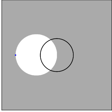
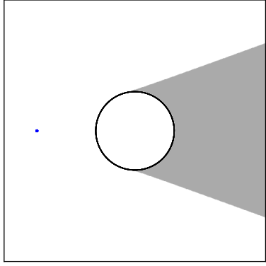
The difference between the shadow function and the visibility function is that the shadow function excludes the obstacles. Although

\tilde{\xi}(x,x_{0})=\max\{-\phi(x),\psi(x,x_{0})\}

looks like a candidate shadow function, it is not correct. In particular

\{x|\tilde{\xi}(x,x_{0})=0\}

includes the portion of the obstacle boundary visible to $x_{0}$ .

Figure 1 summarizes the relevant level set functions used in this work.

3 Value function from HJI equation

Without loss of generality, we formulate the two player game, with a single pursuer and single evader. The domain $\Omega\subseteq\mathbb{R}^{d}$ consists of obstacles and free space: $\Omega=\Omega_{\text{obs}}\cup\Omega_{\text{free}}$ . Consider a pursuer and evader whose positions at a particular time instance are given by ${P},{E}:[0,\infty)\to\Omega_{\text{free}}$ , respectively. Let $A:=S^{d-1}\cup\{{\bf 0}\}$ be the compact set of control values. The feedback controls map the players’ positions to a control value:

\displaystyle{\sigma_{P}},{\sigma_{E}}\in{\mathcal{A}}:=\{\sigma:\Omega_{\text{free}}\times\Omega_{\text{free}}\to A\ |\ \sigma\text{ measurable}\},

(10)

where ${\mathcal{A}}$ is the set of admissible controls. The players move with velocities ${f_{P}},{f_{E}}:\Omega\to[0,\infty)$ according to the dynamics

	$\displaystyle\dot{{P}}(t)$	$\displaystyle={f_{P}}({P}(t)){\sigma_{P}}({P}(t),{E}(t))\qquad$	$\displaystyle\dot{{E}}(t)$	$\displaystyle={f_{E}}({E}(t)){\sigma_{E}}({P}(t),{E}(t))$		(11)
	$\displaystyle{P}(0)$	$\displaystyle={{P}^{0}}\qquad$	$\displaystyle{E}(0)$	$\displaystyle={{E}^{0}}$		(11)

For clarity of notation, we will omit the dependence of the controls on the players’ positions. For simplicity, we assume velocities are isotropic, meaning they do not depend on the controls. In real-world scenarios, this may not be the case. For example, an airplane’s dynamics might be constrained by its momentum and turning radius.

As a slight relaxation, we consider the finite-horizon version of the game, where the pursuers win if they can prolong the game past a time threshold $T$ . Let $\mathcal{T_{\text{end}}}:=\{({P}(\cdot),{E}(\cdot))|\xi({P}(\cdot),{E}(\cdot))\leq 0\}$ be the end-game set of losing positions, where $\xi$ is the shadow function defined in section 2. Define the payoff function

\displaystyle\mathcal{J}[{{P}^{0}},{{E}^{0}},t,{\sigma_{P}},{\sigma_{E}}]:=\inf\{0\leq\tau\leq t|({P}(\tau),{E}(\tau))\in\mathcal{T_{\text{end}}}\},

(12)

where $\mathcal{J}[{{P}^{0}},{{E}^{0}},t,{\sigma_{P}},{\sigma_{E}}]:=t$ if the set $({P}(\tau),{E}(\tau))\in\mathcal{T_{\text{end}}}$ is empty. The payoff is the minimum time-to-occlusion for given set initial positions and controls. Define the finite-horizon value function as:

\displaystyle V({{P}^{0}},{{E}^{0}},t)=\sup_{{\sigma_{P}}\in{\mathcal{A}}}\inf_{{\sigma_{E}}\in{\mathcal{A}}}\mathcal{J}[{{P}^{0}},{{E}^{0}},t,{\sigma_{P}},{\sigma_{E}}]

(13)

The value function describes the length of the game played to time $t$ , starting from all pairs of initial positions, and assuming optimal controls. We are interested in $V({{P}^{0}},{{E}^{0}},T)$ for a sufficiently large $T$ , which characterizes the set of initial positions from which the pursuers can maintain visibility of the evaders for at least $T$ time units. As $T\to\infty$ , we recover the infinite-horizon value function.

By using the principle of optimality and Taylor expansion, one can derive the Hamilton-Jacobi-Isaacs equation [1, 11, 12]:

$\displaystyle V_{t}+\inf_{{\sigma_{E}}\in A}\sup_{{\sigma_{P}}\in A}\{-\nabla_{P}V\cdot{\sigma_{P}}-\nabla_{E}V\cdot{\sigma_{E}}\}$	$\displaystyle=1\ ,$	$\displaystyle\text{ on }\Omega_{\text{free}}\setminus\mathcal{T_{\text{end}}}$	(14)
$\displaystyle V({P},{E},0)$	$\displaystyle=0$
$\displaystyle V({P},{E},t)$	$\displaystyle=0\ ,$	$\displaystyle({P},{E})\in\mathcal{T_{\text{end}}}$
$\displaystyle V({P},{E},t)$	$\displaystyle=\infty\ ,$	$\displaystyle{P}\text{ or }{E}\in\Omega_{\text{obs}}$

It has been shown the value function is the viscosity solution [1, 11, 12] to (14). For isotropic controls, this simplifies to the following Eikonal equation:

$\displaystyle V_{t}-{f_{P}}\|\nabla_{P}V\|+{f_{E}}\|\nabla_{E}V\|$	$\displaystyle=1\ ,$	$\displaystyle\text{ on }\Omega_{\text{free}}\setminus\mathcal{T_{\text{end}}}$	(15)
$\displaystyle V({P},{E},0)$	$\displaystyle=0$
$\displaystyle V({P},{E},t)$	$\displaystyle=0\ ,$	$\displaystyle({P},{E})\in\mathcal{T_{\text{end}}}$
$\displaystyle V({P},{E},t)$	$\displaystyle=\infty\ ,$	$\displaystyle{P}\text{ or }{E}\in\Omega_{\text{obs}}$

The optimal controls can be recovered by computing the gradient of the value function:

\displaystyle{\sigma_{P}}

\displaystyle=\frac{\nabla_{P}V}{|\nabla_{P}V|}\ ,\qquad{\sigma_{E}}=-\frac{\nabla_{E}V}{|\nabla_{E}V|}\ .

(16)

3.1 Algorithm

Following the ideas in [40], we discretize the gradient using upwind scheme as follows. Let ${P}_{i,j},{E}_{k,l}\in\Omega_{\text{free}}$ be the discretized positions with grid spacing $h$ . Denote $V_{i,j,k,l}$ as the numerical solution to (15) for initial positions ${P}_{i,j},{E}_{k,l}$ . We estimate the gradient using finite difference. For clarity, we will only mark the relevant subscripts, e.g. $V_{i+1}:=V_{i+1,j,k,l}$ .

$\displaystyle{P}_{x^{-}}$	$\displaystyle:=\frac{1}{h}\Big(V_{i}-V_{i-1}\Big),\qquad$	$\displaystyle{E}_{x^{-}}$	$\displaystyle:=\frac{1}{h}\Big(V_{k}-V_{k-1}\Big),$	(17)
$\displaystyle{P}_{x^{+}}$	$\displaystyle:=\frac{1}{h}\Big(V_{i+1}-V_{i}\Big),\qquad$	$\displaystyle{E}_{x^{+}}$	$\displaystyle:=\frac{1}{h}\Big(V_{k+1}-V_{k}\Big),$
$\displaystyle{P}_{y^{-}}$	$\displaystyle:=\frac{1}{h}\Big(V_{j}-V_{j-1}\Big),\qquad$	$\displaystyle{E}_{y^{-}}$	$\displaystyle:=\frac{1}{h}\Big(V_{l}-V_{l-1}\Big),$
$\displaystyle{P}_{y^{+}}$	$\displaystyle:=\frac{1}{h}\Big(V_{j+1}-V_{j}\Big),\qquad$	$\displaystyle{E}_{y^{+}}$	$\displaystyle:=\frac{1}{h}\Big(V_{l+1}-V_{l}\Big).$

Let $a^{-}:=-\min(0,a)$ and $a^{+}:=\max(0,a)$ . Define

\displaystyle{\text{sgn}}\max(a,b)

\displaystyle:=\begin{cases}a^{+}&\text{ if }\max(a^{+},b^{-})=a^{+}\\ -b^{-}&\text{ if }\max(a^{+},b^{-})=b^{-}\\ \end{cases}

(18)

and

$\displaystyle\partial{P}_{x}V$	$\displaystyle={\text{sgn}}\max({P}_{x^{+}},{P}_{x^{-}})$	(19)
$\displaystyle\partial{P}_{y}V$	$\displaystyle={\text{sgn}}\max({P}_{y^{+}},{P}_{y^{-}})$
$\displaystyle\partial{E}_{x}V$	$\displaystyle={\text{sgn}}\max({E}_{x^{-}},{E}_{x^{+}})$
$\displaystyle\partial{E}_{y}V$	$\displaystyle={\text{sgn}}\max({E}_{y^{-}},{E}_{y^{+}})$

Finally, the desired numerical gradients are

	$\displaystyle\|\nabla_{P}V\|$	$\displaystyle=\Big((\partial{P}_{x}V)^{2}+(\partial{P}_{y}V)^{2}\Big)^{1/2}$		(20)
	$\displaystyle\|\nabla_{E}V\|$	$\displaystyle=\Big((\partial{E}_{x}V)^{2}+(\partial{E}_{y}V)^{2}\Big)^{1/2}$		(20)

Then we have a simple explicit scheme.

\displaystyle V^{n+1}=V^{n}+\Delta t(1+{f_{P}}|\nabla_{P}V|-{f_{E}}|\nabla_{E}V|)

(21)

The CFL conditions dictate that the time step $\Delta t$ should be

\displaystyle\Delta t\leq\frac{h}{16\max({f_{P}},{f_{E}})}

(22)

For a given environment, we precompute the value function by iteration until convergence. During play time, we initialize ${{P}^{0}},{{E}^{0}}$ and compute the optimal trajectories according to (16) using $\Delta t$ time increments.

3.1.1 Boundary conditions

The obstacles appear in the HJI equation as boundary conditions. However, direct numerical implementation leads to artifacts near the obstacles. Instead, we model the obstacles by setting the velocities to be small inside obstacles. We regularize the velocities by adding a smooth transition [36]:

\displaystyle v_{\epsilon}(x)

\displaystyle=\begin{cases}v(x)&\phi(x)>0\\ v_{\text{min}}+\frac{v(x)-v_{\text{min}}}{2}\Big[\cos\Big(\frac{\phi(x)\pi}{2\epsilon}\Big)+1\Big]&\phi(x)\in[-2\epsilon,0]\\ v_{\text{min}}&\phi(x)<-2\epsilon\end{cases}

(23)

where $\phi$ is the signed distance function to the obstacle boundaries. In the numerical experiments, we use $\epsilon=16\Delta x$ and $v_{\text{min}}=1/100$ .

3.2 Numerical results

Stationary pursuer

We verify that the scheme converges numerically for the case in which the pursuer is stationary. When ${f_{P}}=0$ , the HJI equation (15) becomes the time-dependent Eikonal equation:

$\displaystyle V_{t}+{f_{E}}\|\nabla_{E}V\|$	$\displaystyle=1\qquad$	$\displaystyle\text{ on }\Omega_{\text{free}}\setminus\mathcal{T_{\text{end}}}$	(24)
$\displaystyle V({P},{E},0)$	$\displaystyle=0$
$\displaystyle V({P},{E},t)$	$\displaystyle=0$	$\displaystyle\qquad({P},{E})\in\mathcal{T_{\text{end}}}$

In particular, for sufficiently large $t$ , the value function reaches a steady state, and satisfies the Eikonal equation:

	$\displaystyle{f_{E}}\|\nabla_{E}V\|$	$\displaystyle=1\qquad$	$\displaystyle\text{ on }\Omega_{\text{free}}\setminus\mathcal{T_{\text{end}}}$		(25)
	$\displaystyle V({P},{E})$	$\displaystyle=0$	$\displaystyle\qquad({P},{E})\in\mathcal{T_{\text{end}}}$		(25)

For this special case, the exact solution is known; the solution corresponds to the evader’s travel time to the end-game set $\mathcal{T_{\text{end}}}$ . Also, this case effectively reduces the computational cost from $\mathcal{O}(m^{4})$ to $\mathcal{O}(m^{2})$ , so that we can reasonably compute solutions at higher resolutions.

We consider a $\Omega=[0,1)\times[0,1)$ with a single circular obstacle of radius $0.15$ centered at $(1/2,1/2)$ . The pursuer is stationary at ${P}_{0}=(1/8,1/2)$ . We use $\Delta t=\Delta x/20$ and iterate until the solution no longer changes in the $L_{1}$ sense, using a tolerance of $10^{-5}$ .

We compute the “exact” solution using fast marching method on high resolution grid $M=2048$ . We vary $m$ from $16$ to $1024$ and observe convergence in the $L_{1}$ and $L_{2}$ sense, as seen in Table 1. In Figure 2, we plot the level curves comparing the computed solution at $m=512,1024$ to the “exact” solution. Notice the discrepancies are a result of the difficulty in dealing with boundary conditions. However, these errors decay as the grid is refined.

The case where the evader is stationary is not interesting.

Table 1: Error for the stationary pursuer case, compared to the known solution computed using fast marching method at resolution

M=2048

$m$	$L_{1}$ error	$L_{2}$ error
$16$	$0.08972215$	$0.01288563$
$32$	$0.03177683$	$0.00159669$
$64$	$0.02442984$	$0.00111537$
$128$	$0.01059728$	$0.00021345$
$256$	$0.00515584$	$0.00005214$
$512$	$0.00304322$	$0.00001961$
$1024$	$0.00086068$	$0.00000142$

A circular obstacle

The evader has the advantage in the surveillance-evasion game. It is difficult for the pursuer to win unless it is sufficiently fast. But once it is fast enough, it can almost always win. Define the winning regions for the pursuer and evader, respectively:

	$\displaystyle\mathcal{W}_{P}$	$\displaystyle=\{({P},{E})\|V({P},{E})>T_{\text{max}}\}$		(26)
	$\displaystyle\mathcal{W}_{E}$	$\displaystyle=\{({P},{E})\|V({P},{E})\leq T_{\text{max}}\}$		(27)

Here, we use $T_{\text{max}}=.9T$ to tolerate numerical artifacts due to boundary conditions. In Figure 3, we show how the winning region for a fixed evader/pursuer position changes as the pursuer’s speed increases. Since it is difficult to visualize data in 4D, we plot the slices $V({{P}^{0}},\cdot)$ and $V(\cdot,{{E}^{0}})$ where ${{P}^{0}}={{E}^{0}}=(1/8,1/2)$ . We use $m=64$ , $\Delta t=\Delta x/20$ and iterate until $T=10$ . We fix ${f_{P}}=1$ and compute $V$ for each ${f_{E}}\in\{\frac{1}{3},\frac{1}{2},\frac{2}{3}\}$ . The computation for each value function takes 16 hours.

Figure 4 shows trajectories from several initial positions with various speeds. Interestingly, once the evader is cornered, the optimal controls dictate that it is futile to move. That is, the value function is locally constant.

More obstacles

In Figure 5 we consider a more complicated environment with multiple obstacles. Here, the pursuer is twice as fast as the evader. Although there are many obstacles, the dynamics are not so interesting in the sense that the evader will generally navigate towards a single obstacle. Again, the evader tends to give up once the game has been decided.

Finally, in Figure 6 we show suboptimal controls for the evader. In particular, the evader is controlled manually. Although manual controls do not help the evader win, they lead to more interesting trajectories.

3.3 Discussion

Notice that an optimal trajectory for the pursuer balances distance and visibility. While moving closer to the evader will guarantee that it can’t “get away”, it is not sufficient, since being close leads to more occlussions. On the other hand, moving far away gives better visibility of the environment, but may make it impossible to catch up once E turns the corner.

Although we described the formulation for a single pursuer and evader, the same scheme holds for multiple pursuers and evaders. The end-game set just needs to be modified to take into account the multiple players. That is, the game ends as soon as any evader is occluded from all pursuers. However, the computational complexity of the scheme is $\mathcal{O}(m^{kd})$ which quickly becomes unfeasible even on small grid sizes. At the expense of offline compute time, the game can be played efficiently online. The caveat is that, the value function is only valid for the specific map and velocities computed offline.

4 Locally optimal strategies

As the number of players increases, computing the value function from the HJI equations is no longer tractable. We consider a discrete version of the game, with the aim of feasibly computing controls for games with multiple pursuers and multiple evaders. Each player’s position is now restricted on a grid, and at each turn, the player can move to a new position within a neighborhood determined by its velocity. Players cannot move through obstacles. Formally, define the arrival time function

	$\displaystyle d_{{P}}(x,y)$	$\displaystyle:=\min_{{\sigma_{P}}\in{\mathcal{A}}}\min\{t\|{P}(0)=x,{P}(t)=y\}$		(28)
	$\displaystyle d_{{E}}(x,y)$	$\displaystyle:=\min_{{\sigma_{E}}\in{\mathcal{A}}}\min\{t\|{E}(0)=x,{E}(t)=y\}.$		(28)

The set of valid actions are the positions $y$ which can be reached from $x$ within a $\Delta t$ time increment:

	$\displaystyle A_{{P}}(t)$	$\displaystyle:=\{y\in\Omega_{\text{free}}\|d_{{P}}({P}(t),y)\leq\Delta t\}$		(29)
	$\displaystyle A_{{E}}(t)$	$\displaystyle:=\{y\in\Omega_{\text{free}}\|d_{{E}}({E}(t),y)\leq\Delta t\}.$		(29)

In a $\Delta t$ time step, each player can move to a position

	$\displaystyle{P}(t+\Delta t)\in A_{{P}}(t)$		(30)
	$\displaystyle{E}(t+\Delta t)\in A_{{E}}(t).$		(30)

Analogously, for multiple players, denote the number of pursuers and evaders as $k_{P}$ and $k_{E}$ , respectively. Define

$\displaystyle{{\bf P}}$	$\displaystyle=({P}_{1},\dots,{P}_{k_{P}})$	(31)
$\displaystyle{{\bf E}}$	$\displaystyle=({E}_{1},\dots,{E}_{k_{E}})$
$\displaystyle{\bf A_{{P}}}(t)$	$\displaystyle=\{{{\bf P}}\|{P}_{i}\in A_{{P}}(t)\ ,\ i=1,\dots,k_{P}\}$
$\displaystyle{\bf A_{{E}}}(t)$	$\displaystyle=\{{{\bf E}}\|{E}_{j}\in A_{{E}}(t)\ ,\ j=1,\dots,k_{E}\}$

so that in $\Delta t$ time, each team can move to

	$\displaystyle{{\bf P}}(t+\Delta t)\in{\bf A_{{P}}}(t)$		(32)
	$\displaystyle{{\bf E}}(t+\Delta t)\in{\bf A_{{E}}}(t)$		(32)

The game ends as soon as one evader is occluded from all pursuers. The end-game set is

\displaystyle\mathcal{T_{\text{end}}}=\{({{\bf P}},{{\bf E}})\ |\ \exists\ j:\xi({P}_{i},{E}_{j})\leq 0\text{ for }i=1,\dots,k_{P}\},

(33)

We propose two locally optimal strategies for the pursuer.

4.1 Distance strategy

The trajectories from the section 3 suggest that the pursuer must generally remain close to the evader. Otherwise, the evader can quickly hide behind obstacles. A simple strategy for the pursuer is to move towards the evader:

\displaystyle{P}(t+\Delta t)

\displaystyle=\argmin_{x\in A_{{P}}(t)}d_{{P}}\Big(x,{E}(t)\Big).

(34)

That is, in the time increment $\Delta t$ , the pursuer should pick the action that minimizes its travel time to the evader’s current position at time $t$ .

For the multiplayer game, we propose a variant of the Hausdorff distance, where max is replaced by a sum:

\displaystyle{\bf d_{{P}}}({\bf x,{E}}(t)):=\frac{1}{2}\Big[\sum_{i=1}^{k_{P}}\min_{j}d_{{P}_{i}}\Big(x_{i},{E}_{j}(t)\Big)^{2}\ \Big]^{1/2}+\frac{1}{2}\Big[\sum_{j=1}^{k_{E}}\min_{i}d_{{P}_{i}}\Big(x_{i},{E}_{j}(t)\Big)^{2}\ \Big]^{1/2}.

Informally, the first term encourages each pursuer to be close to an evader, while the second term encourages a pursuer to be close to each evader. The sum helps to prevent ties. The optimal action according to the distance strategy is

\displaystyle{{{\bf P}}(t+\Delta t)}=\argmin_{{\bf x}\in{\bf A_{{P}}}(t)}{\bf d_{{P}}}({\bf x,{E}}(t))

(35)

In the next section, we will use search algorithms to refine policies. Rather than determining the best action, it is useful to quantify the utility of each action. To do so, define $p_{\text{distance}}:\Omega\times\Omega_{\text{free}}\times\dots\times\Omega_{\text{free}}\to\mathbb{R}$ as the policy, which outputs a probability the agent should take an action, conditioned on the current player positions. We normalize using the softmax function to generate the policy:

	$\displaystyle\alpha$	$\displaystyle=\Big[\displaystyle{\sum_{{\bf x}\in{\bf A_{{P}}}(t)}}e^{-{\bf d_{{P}}}({\bf x},{\bf{E}}(t))}\Big]^{-1}$		(36)
	$\displaystyle p_{\text{distance}}\big({\bf x}\|({\bf{P}}(t),{\bf{E}}(t))\big)$	$\displaystyle=\begin{cases}\alpha e^{-{\bf d_{{P}}}({\bf x},{\bf{E}}(t))}&{\bf x}\in{\bf A_{{P}}}(t)\\ 0&\text{otherwise}\end{cases}$		(36)

For the discrete game with $\Delta t$ time increments, one can enumerate the possible positions for each ${P}_{i}$ and evaluate the travel time to find the optimal control. The arrival time function $d_{{P}_{i}}(\cdot,{E}_{j}(t))$ to each ${E}_{j}$ at the current time $t$ can be precomputed in $\mathcal{O}(m^{d})$ time. In the general case, where each pursuer may have a different velocity field ${f_{P}}_{i}$ , one would need to compute $k_{P}$ arrival time functions. If $a_{\Delta t}(P_{i})$ is the max number of possible actions each pursuer can make in $\Delta t$ increment, then the total computational complexity for one move is

O\Big(k_{P}k_{E}m^{d}+\prod_{i=1}^{k_{P}}a_{\Delta_{t}}(P_{i})\Big).

For the special case when the pursuers have the same ${f_{P}}$ , the complexity reduces to

O\Big(k_{E}m^{d}+\prod_{i=1}^{k_{P}}a_{\Delta_{t}}(P_{i})\Big).

4.2 Shadow strategy

Recall that, for a stationary pursuer, the value function for the evader becomes the Eikonal equation:

	$\displaystyle{f_{E}}\|\nabla_{E}V\|$	$\displaystyle=1\qquad$	$\displaystyle\text{ on }\Omega_{\text{free}}\setminus\mathcal{T_{\text{end}}}$		(37)
	$\displaystyle V({P},{E})$	$\displaystyle=0$	$\displaystyle\qquad({P},{E})\in\mathcal{T_{\text{end}}},$		(37)

whose solution is the travel time to the shadow set. Define the time-to-occlusion as

\displaystyle\tau_{{E}}({P},{E}^{0}):=\min_{{\sigma_{E}}\in{\mathcal{A}}}\min\{t\geq 0\ |\ {E}(0)={E}^{0}\ ,\ ({P},{E}(t))\in\mathcal{T_{\text{end}}}\ \}.

(38)

It is the shortest time in which an evader at ${E}^{0}$ can be occluded from a stationary pursuer at ${P}$ . Thus, a reasonable strategy for the evader is to pick the action which brings it closest to the shadow formed by the pursuer’s position:

\displaystyle{E}(t+\Delta t)=\argmin_{y\in A_{{E}}(t)}\tau_{{E}}({P}(t),y).

(39)

A conservative strategy for the pursuer, then, is to maximize time-to-occlusion, assuming that the evader can anticipate its actions:

	$\displaystyle\tau_{{E}}^{\ast}(x,{E}(t))$	$\displaystyle=\min_{y\in A_{{E}}(t)}\tau_{{E}}(x,y)$		(40)
	$\displaystyle{P}(t+\Delta t)$	$\displaystyle=\argmax_{x\in A_{{P}}(t)}\tau_{{E}}^{\ast}(x).$		(41)

Remark: The strategy (41) is a local variant of the static value function proposed in [36]. In that paper, they suggest using the static value function for feedback controls by moving towards the globally optimal destination, and then recomputing at $\Delta t$ time intervals. Here, we use the locally optimal action.

For multiple players, the game ends as soon as any evader is hidden from all pursuers. Define the time-to-occlusion for multiple players:

\displaystyle{\bf\uptau_{{E}}}({{{\bf P}}},{{\bf E}}^{0}):=\min_{{\sigma_{E}}_{i}\in{\mathcal{A}}}\min\{t\geq 0\ |\ {{\bf E}}(0)={{\bf E}}^{0}\ ,\ ({{\bf P}},{{\bf E}}(t))\in\mathcal{T_{\text{end}}}\ \}.

(42)

Then, the strategy should consider the shortest time-to-occlusion among all possible evaders’ actions in the $\Delta t$ time increment:

	$\displaystyle{\bf\uptau_{{E}}}^{\ast}({\bf x},{\bf{E}}(t))$	$\displaystyle:=\min_{{\bf y}\in{\bf A_{{E}}}(t)}{\bf\uptau_{{E}}}({\bf x},{\bf y})$		(43)
	$\displaystyle{{\bf P}}(t+\Delta t)$	$\displaystyle=\argmax_{{\bf x}\in{\bf A_{{P}}}(t)}{\bf\uptau_{{E}}}^{\ast}({\bf x},{\bf{E}}(t)).$		(43)

The corresponding shadow policy is:

	$\displaystyle\alpha$	$\displaystyle=\Big[\displaystyle{\sum_{x\in{\bf A_{{P}}}(t)}}e^{{\bf\uptau_{{E}}}^{\ast}({\bf x},{\bf{E}}(t))}\Big]^{-1}$		(44)
	$\displaystyle p_{\text{shadow}}\big({\bf x}\|({\bf{P}}(t),{\bf{E}}(t))\big)$	$\displaystyle=\begin{cases}\alpha e^{{\bf\uptau_{{E}}}^{\ast}({\bf x},{\bf{E}}(t))}&{\bf x}\in{\bf A_{{P}}}(t)\\ 0&\text{otherwise}\end{cases}$		(44)

This strategy is computationally expensive. One can precompute the arrival time to each evader by solving an Eikonal equation $\mathcal{O}(m^{d})$ . For each combination of pursuer positions, one must compute the joint visibility function and corresponding shadow function $\mathcal{O}(m^{d})$ . Then the time-to-occlusion can be found by evaluating the precomputed arrival times to find the minimum within the shadow set $\mathcal{O}(m^{d})$ . The computational complexity for one move is

\displaystyle O\Big(k_{E}m^{d}+m^{d}\cdot\prod_{i=1}^{k_{P}}a_{\Delta t}(P_{i})\Big).

(45)

One may also consider alternating minimization strategies to achieve

\displaystyle O\Big(k_{E}m^{d}+m^{d}\cdot\sum_{i=1}^{k_{P}}a_{\Delta t}(P_{i})\Big),

(46)

though we leave that for future work.

Blend strategy

We have seen from 3 that optimal controls for the pursuer balance the distance to, and visibility of, the evader. Thus a reasonable approach would be to combine the distance and shadow strategies. However, it is not clear how they should be integrated. One may consider a linear combination, but the appropriate weighting depends on the game settings and environment. Empirically, we observe that the product of the policies provides promising results across a range of scenarios. Specifically,

\displaystyle p_{\text{blend}}\propto p_{\text{shadow}}\cdot p_{\text{distance}}

(47)

4.3 Numerical results

We present some representative examples of the local policies. First, we consider the game with a circular obstacle, a single purser and single evader whose speeds are ${f_{P}}=3$ and ${f_{E}}=2$ , respectively. Figure 7 illustrates the typical trajectories for each policy. In general, the distance strategy leads the pursuer into a cat-and-mouse game the with evader; the pursuer, when close enough, will jump to the evader’s position at the previous time step. The shadow strategy keeps the pursuer far away from obstacles, since this allows it to steer the shadows in the fastest way. The blend strategy balances the two approaches and resembles the optimal trajectories based on the HJI equation in section 3.

Next, we highlight the advantages of the shadow strategy with a 2 pursuer, 2 evader game on a map with two crescent-shaped obstacles. The pursuer and evader speeds are ${f_{P}}=4$ and ${f_{E}}=2$ , respectively. The openness of the environment creates large occlusions. The pursuers use the shadow strategy to cooperate and essentially corner the evaders. Figure 8 shows snapshots of the game. The distance strategy loses immediately since the green purser does not properly track the orange evader.

We present cases where the distance and shadow strategy fail in Figure 9. The evader tends to stay close to the obstacle, since that enables the shortest path around the obstacle. Using the distance strategy, the pursuer agressively follows the evader. The evader is able to counter by quickly jumping behind sharp corners. On the other hand, the shadow strategy moves the pursuer away from obstacles to reduce the size of shadows. As a consequence, the pursuer will generally be too far away from the evader and eventually lose. In environments with many nonconvex obstacles, both strategies will fail.

Finally, we show that blending the shadow and distance strategies is very effective in compensating for the shortcomings of each individual policy. The pursuers are able to efficiently track the evaders while maintain a safe distance. Figure 10 shows an example with 2 pursuers and 2 evaders on a map with multiple obstacles, where ${f_{P}}=3$ and ${f_{E}}=2$ .

5 Learning the pursuer policy

We propose a method for learning optimal controls for the pursuer, though our methods can be applied to find controls for the evader as well. Again, we consider a discrete game, where each player’s position is restricted on a grid, and at each turn, the player can move to a new position within a neighborhood determined by their velocity. All players move simultaneously. The game termination conditions are checked at the end of each turn.

We initialize a neural network which takes as input any game state, and produces a policy and value pair. The policy is probability distribution over actions. Unlike in section 3, the value, in this context, is an estimate of the likely winner given the input state.

Initially the policy and value estimates are random. We use Monte Carlo tree search to compute refined policies. We play the game using the refined policies, and train the neural network to learn the refined policies. By iterating in this feedback loop, the neural network continually learns to improve its policy and value estimates. We train on games in various environments and play games on-line on maps that were were not seen during the training phase.

5.1 Monte Carlo tree search

In this section, we review the Monte Carlo tree search algorithm, which allows the agent to plan ahead and refine policies. For clarity of notation, we describe the single pursuer, single evader scenario, but the method applies to arbitrary number of players.

Define the set of game states $\mathcal{S}:=\{({P},{E})\in\Omega_{\text{free}}\times\Omega_{\text{free}}\}$ so that each state $s\in\mathcal{S}$ characterizes the position of the players. Let $\mathcal{A}\subseteq\Omega_{\text{free}}$ be the set of actions. Let $T(s,a):\mathcal{S}\times\mathcal{A}\to\mathcal{S}$ be the transition function which outputs the state resulting from taking action $a$ at state $s$ . Let ${f}:\mathcal{S}\to\mathbb{R}^{m^{d}}\times[-1,1]$ be an evaluator function which takes the current state as input and provides a policy and value estimate: ${f}(s)=(\vec{p},v)$ . Formally, Monte Carlo tree search is mapping takes as input the current state $s_{0}$ , the evaluator function ${f}$ , and a parameter $M$ indicating the number of search iterations: $\text{MCTS}(s_{0},{f};M)$ . It outputs a refined policy $\vec{\pi}^{\ast}$ .

Algorithm 1 summarizes the MCTS algorithm. At a high level, MCTS simulates game play starting from the current state, keeping track of nodes it has visited during the search. Each action is chosen according to a formula $U(s,a)$ which balances exploration and exploitation. Simulation continues until the algorithm reaches a leaf node $s_{n}$ , a state which has not previously been visited. At this point, we use the evaluator function ${f}(s_{n})=(\vec{p},v)$ to estimate a policy and value for that leaf node. The value $v$ is propagated to all parent nodes. One iteration of MCTS ends when it reaches a leaf node. MCTS keeps track of statistics that help guide the search. In particular

•

$N(s,a)$ : the number of times the action $a$ has been selected from state $s$
•

$W(s,a)$ : the cumulative value estimate for each state-action pair
•

$Q(s,a)$ : the mean value estimate for each state-action pair
•

$P(s,a)=(1-\varepsilon)p(a|s)+\varepsilon\eta$ : the prior policy, computed by evaluating ${f}$ . Dirichlet noise $\eta$ is added to allow a chance for each move to be chosen.
•

$U(s,a)=Q(s,a)+P(s,a)\frac{\sqrt{\sum_{b}N(s,b)}}{1+N(s,a)}$ is the upper confidence bound [27]. The first term exploits moves with high value, while the second term encourages moves that have not selected.

When all $M$ iterations are completed, the desired refined policy is proportional to $N(s_{0},a)^{1/\tau}$ , where $\tau$ is a smoothing term.

Algorithm 1 Monte Carlo tree search:

\text{MCTS}(s_{0},{f},M)

N(s,a)\leftarrow 0

Q(s,a)\leftarrow 0

W(s,a)\leftarrow 0

visited =

\{\emptyset\}

for

i=1,\dots,M

n\leftarrow 0

while

s_{n}\notin

visited do

\sum_{b}N(s_{n},b)>0

then

a_{n}^{\ast}=\arg\max_{a}Q(s_{n},a)+P(s_{n},a)\frac{\sqrt{\sum_{b}N(s_{n},b)}}{1+N(s_{n},a)}

else

a_{n}^{\ast}=\arg\max_{a}P(s_{n},a)

end if

s_{n+1}=T(s_{n},a_{n}^{\ast})

n\leftarrow n+1

end while

(p,v)={f}(s_{n})

P(s_{n},a)=(1-\varepsilon)p(a|s_{n})+\varepsilon\eta

visited.append(

s_{n}

)

for

j=0,\dots,n-1

N(s_{j},a)\leftarrow N(s_{j},a_{j}^{\ast})+1

W(s_{j},a)\leftarrow W(s_{j},a_{j}^{\ast})+v

Q(s_{j},a)\leftarrow Q(s_{j},a_{j}^{\ast})/N(s_{j},a_{j}^{\ast})

end for

\pi^{\ast}(a|s_{0})=N(s_{0},a)^{1/\tau}/\sum_{b}N(s_{0},b)^{1/\tau}

return

\pi^{\ast}

5.2 Policy and value network

We use a convolutional neural network which takes in the game state and produces a policy and value estimate. Although the state can be completely characterized by the positions of the players and the obstacles, the neural network requires more context in order to be able to generalize to new environments. We provide the following features as input to the neural network, each of which is an $m\times m$ image:

•

Obstacles as binary image
•

Player positions, a separate binary image for each player
•

Joint visibility of all pursuers, as a binary image
•

Joint shadow boundaries of all pursuers
•

Visibility from each pursuer’s perspective, as a binary image
•

Shadow boundary from each pursuer’s perspective
•

Valid actions for each player, as a binary image
•

Each evader’s policy according to (39)

AlphaZero [31] suggests that training the policy and value networks jointly improves performance. We use a single network based on U-Net [26], which splits off to give output policy and value.

The input is $m\times m\times C_{\text{in}}$ , where $C_{\text{in}}=2+4k_{P}+2k_{E}$ and $k_{P},k_{E}$ are the number of pursuers and evaders, respectively. The U-Net consists of $\log_{2}(m)+1$ down-blocks, followed by the same number of up-blocks. All convolution layers in the down-blocks and up-blocks use size 3 kernels. Each down-block consists of input, conv, batch norm, relu, conv, batch norm, residual connection from input, relu, followed by downsampling with stride 2 conv, batch norm, and relu. A residual connection links the beginning and end of each block, before downsampling. The width of each conv layer in the $l^{th}$ down-block is $l\cdot C_{\text{in}}$ . Each up-block is the same as the down-block, except instead of downsampling, we use bilinear interpolation to upsample the image by a factor of 2. The upsampled result is concatenated with the predownsampled output from the corresponding (same size) down-block, followed by conv, batch norm, relu. The width of each conv layer in the up-block is same as those in the down-block of corresponding size.

Then, the network splits into a policy and value head. The policy head consists of $1\times 1$ conv with width 8, batch norm, relu, and $1\times 1$ conv with width $k_{P}$ . The final activation layer is a softmax to output $p\in\mathbb{R}^{m\times m\times k_{P}}$ , a policy for each pursuer. The value head is similar, with $1\times 1$ conv with width 8, batch norm, relu, and $1\times 1$ conv with width 1. The result passes through a tanh activation and average pooling to output a scalar $v\in[-1,1]$ .

5.3 Training procedure

Since we do not have the true value and policy, we cannot train the networks in the usual supervised fashion. Instead, we use MCTS to generate refined policies, which serve as the training label for the policy network. Multiple games are played with actions selected according to MCTS refined policies. The game outcomes act as the label for the value for each state in the game. We train over various maps consisting of 2-7 obstacles, including circles, ellipses, squares, and tetrahedrons.

More specifically, let ${f}_{\theta}(s)$ be the neural network parameterized by $\theta$ , which takes a state $s$ as input, and outputs a policy $\vec{\pi}_{\theta}(s)$ and value $v_{\theta}(s)$ . Let $s_{j}(0)$ be the initial positions. For $j=1,\dots,J$ , play the game using MCTS:

	$\displaystyle\vec{\pi}_{j}(a\|s_{j}(k))$	$\displaystyle=\text{MCTS}(s_{j}(k),f_{\theta};M)$		(48)
	$\displaystyle s_{j}(k+1)$	$\displaystyle=\arg\max_{a}\vec{\pi}_{j}^{\ast}(a\|s_{j}(k))$		(49)

for $k=0,\dots,K_{j}$ . The game ends at

\displaystyle K_{j}=\inf\{k|s_{j}(k)\in\mathcal{T}_{\text{end}}\}

(50)

Then the ”true” policy and value are

	$\displaystyle\vec{\pi}_{j}^{\ast}(k)$	$\displaystyle=\vec{\pi}_{j}(\cdot\|s_{j}(k))$		(51)
	$\displaystyle v^{\ast}_{j}(k)$	$\displaystyle=\begin{cases}1&K_{j}>K_{\text{max}}\\ -1&\text{otherwise}\end{cases}$		(52)

The parameters $\theta$ of the neural network are updated by stochastic gradient descent (SGD) on the loss function:

$\displaystyle\min_{\theta}\sum_{j=1}^{J}\sum_{k=0}^{K_{j}}L_{\text{policy}}$	$\displaystyle\Big(\vec{\pi}_{\theta}(s_{j}(k)),\vec{\pi}_{j}^{\ast}(k)\Big)+L_{\text{value}}\Big(v_{\theta}(s_{j}(k)),v_{j}^{\ast}(k)\Big)$	(53)
$\displaystyle L_{\text{policy}}(\vec{p},\vec{q})$	$\displaystyle=-\vec{p}\cdot\log\vec{q}$
$\displaystyle L_{\text{value}}(p,q)$	$\displaystyle=(p-q)^{2}$

We use a learning rate of $0.001$ and the Adam optimizer [19].

5.4 Numerical results

A key difficulty in learning a good policy for the pursuer is that it requires a good evader. If the evader is static, then the pursuer can win with any random policy.

During training and evaluation, the game is played with the evader moving according to (39). Although all players move simultaneously, our MCTS models each team’s actions sequentially, with the pursuers moving first. This is conservative towards the pursuers, since the evaders can counter.

We train using a single workstation with 2 Intel Xeon CPU E5-2620 v4 2.10GHz processors and a single NVidia 1080-TI GPU. For simplicity, ${f_{P}}$ and ${f_{E}}$ are constant, though it is straightforward to have spatially varying velocity fields. We use a gridsize of $m=16$ . We set $K_{\text{max}}=100$ and $M=1000$ MCTS iterations per move. One step of training consists of playing $J=64$ games and then training the neural network for 1 epoch based on training data for the last 10 steps of training. Self-play game data is generated in parallel, while network training is done using the GPU with batch size 128. The total training time is 1 day.

The training environments consist of between 2 to 6 randomly oriented obstacles, each uniformly chosen from the set of ellipses, diamonds, and rectangles. We emphasize that the environments shown in the experiments are not in the training set.

We compare our trained neural network against uniform random and dirichlet noise-based policies, as well as the local policies from section 4. In order to draw a fair comparison, we make sure each action requires the same amount of compute time. Each MCTS-based move in the 2 player game takes 4 secs while the multiplayer game takes about 10 secs per move, on average. Since the noise-based policies require less overhead, they are able to use more MCTS iterations. The shadow strategies become very expensive as more players are added. For the 1v1 game, we use $\hat{M}=1000$ , while the 2v2 game can only run for $\hat{M}=250$ in the same amount of time as the Neural Net. Specifically,

•

Distance strategy
•

Shadow strategy
•

Blend strategy
•

$\text{MCTS}(\cdot,{f}_{\text{distance}},1000)$ where ${f}_{\text{distance}}(s)=(p_{\text{distance}},0)$ .
•

$\text{MCTS}(\cdot,{f}_{\text{shadow}},\hat{M})$ where ${f}_{\text{shadow}}(s)=(p_{\text{shadow}},0)$ .
•

$\text{MCTS}(\cdot,{f}_{\text{blend}},\hat{M})$ where ${f}_{\text{blend}}(s)=(p_{\text{blend}},0)$ .
•

$\text{MCTS}(\cdot,{f}_{\mu},2000)$ where ${f}_{\nu}(s)=(\text{Uniform},0)$ .
•

$\text{MCTS}(\cdot,{f}_{\eta},2000)$ where ${f}_{\eta}(s)=(\text{Dir}(0.3),0)$ .
•

$\text{MCTS}(\cdot,{f}_{\theta},1000)$ where ${f}_{\theta}$ is the trained Neural Network

Two players

As a sanity check, we show an example on a single circular obstacle with a single pursuer and single evader. As we saw from the previous section, the pursuer needs to be faster in order to have a chance at winning. We let ${f_{P}}=2$ and ${f_{E}}=1$ . Figure 11 shows an example trajectory using Neural Net. The neural network model gives reasonable policies. Figure 12 shows an adversarial human evader playing against the Neural Net pursuer, on a map with two obstacles. The pursuer changes strategies depending on the shape of the obstacle. In particular, near the corners of the ”V” shape, it maintains a safe distance rather than blindly following the evader.

In order to do a more systematic comparison, we run multiple games over the same map and report the game time statistics for each method. We fix the pursuer’s position at $(1/2,1/4)$ and vary the evader’s initial location within the free space. Figure 13 shows the setup for the two maps considered for the statistical studies in this section. One contains a single circle in the center, as we have seen previously. The other one contain 5 circular obstacles, though the one in the center has some extra protrusions.

Figure 14 shows an image corresponding the the length of the game for each evader position; essentially, it is a single slice of the value function for each method. Table 2 shows the number of games won. Shadow strategy particularly benefits from using MCTS for policy improvements, going from 16% to 67.15% win rate. Our neural network model outperforms the rest with a 70.8% win rate.

Table 2: Game statistics for the 1 pursuer vs 1 evader game with 5 circular obstacles, where

{f_{P}}=2

and

{f_{E}}=1

Method	Win % (137 games)	Average game time
Distance	52.55	53.56
Shadow	16.06	22.36
Blend	63.50	64.45
MCTS( $\cdot$ , Distance; 1000)	55.47	62.40
MCTS( $\cdot$ , Shadow; 1000)	67.15	69.45
MCTS( $\cdot$ , Blend; 1000)	58.39	63.27
MCTS( $\cdot$ , Uniform; 2000)	60.58	65.84
MCTS( $\cdot$ , Dirichlet; 2000)	65.69	69.02
MCTS( $\cdot$ , Neural Net; 1000)	70.80	71.61

Multiple players

Next, we consider the multiplayer case with 2 pursuers and 2 evaders on a circular obstacle map where ${f_{P}}=2$ and ${f_{E}}=2$ . Even on a $16\times 16$ grid, the computation of the corresponding feedback value function would take several days. Figure 15 shows a sample trajectory. Surprisingly, the neural network has learned a smart strategy. Since there is only a single obstacle, it is sufficient for each pursuer to guard one opposing corner of the map. Although all players have the same speed, it is possible to win.

Figure 16 shows a slice of the value function, where 3 players’ positions are fixed, and one evader’s position varies. Table 3 shows the game statistics. Here, we see some deviation from the baseline. As the number of players increase, the number of actions increases. It is no longer sufficient to use random sampling. The neural network is learning useful strategies to help guide the Monte Carlo tree search to more significant paths. The distance and blend strategies are effective by themselves. MCTS helps improve performance for Distance. However, 250 iterations is not enough to search the action space, and actually lead to poor performance for Blend and Shadow. For this game setup, MCTS(Distance,1000) performs the best with a 73.5% win rate, followed by Blend with 65.4% and Neural Net with 59.9%. Although the trained network is not the best in this case, the results are very promising. We want to emphasize that the model was trained with no prior knowledge. Given enough offline time and resources, we believe the proposed approach can scale to larger grids and learn more optimal policies than the local heuristics.

Table 3: Game statistics for the 2 pursuer vs 2 evader game with a circular obstacle.

Method	Win % (162 games)	Average game time
Distance	56.8	58.8
Shadow	46.3	50.1
Blend	65.4	67.9
MCTS( $\cdot$ , Distance; 1000)	73.5	76.6
MCTS( $\cdot$ , Shadow; 250)	40.7	44.5
MCTS( $\cdot$ , Blend; 250)	00.0	4.4
MCTS( $\cdot$ , Uniform; 2000)	00.0	5.3
MCTS( $\cdot$ , Dirichlet; 2000)	27.8	32.8
MCTS( $\cdot$ , Neural Net; 1000)	59.9	61.7

Figure 17 shows a comparison of the depth of search for $M=1000$ MCTS iterations. Specifically, we report depth of each leaf node, as measured by game time. To be fair, we allow the uniform and dirichlet baselines to run for 2000 MCTS iterations to match the runtime needed for 1 move. Also, the shadow strategies are extremely costly, and can only run 250 MCTS iterations in the same amount of time. However, we show the statistics for $M=1000$ to gain better insights. Ideally, a good search would balance breadth and depth. The neural network appears to search further than the baselines. Of course, this alone is not sufficient to draw any conclusions. For example, a naive approach could be a depth-first search.

In Figure 18, we show a similar chart for the single pursuer, single evader game with a circular obstacle. In this case, the game is relatively easy, and all evaluator functions are comparable.

Figure 17: Histogram of leaf node depth for MCTS using various evaluator functions for the multiplayer game around a circular obstacle. The colors show increments of 100 iterations. The multiplayer game has a much larger action space, making tree search difficult. The neural network appears to search deeper into the tree.

Figure 18: Histogram of leaf node depth for MCTS using various evaluator functions for the single pursuer vs single evader game around a circular obstacle. The colors show increments of 100 iterations. The game is relatively easy and thus all algorithms appear comparable. Note that Uniform and Dirichlet are allowed 2000 MCTS iterations, since they require less overhead to run.

6 Conclusion and future work

We proposed three approaches for approximating optimal controls for the surveillance-evasion game. When there are few players and the grid size is small, one may compute the value function via the Hamilton-Jacobi-Isaacs equations. The offline cost is immense, but on-line game play is very efficient. The game can be played on the continuously in time and space, since the controls can be interpolated from the value function. However, the value function must be recomputed if the game settings, such as the obstacles or player velocities, change.

When there are many players, we proposed locally optimal strategies for the pursuer and evader. There is no offline preprocessing. All computation is done on-line, though the computation does not scale well as the velocities or number of pursuers increases. The game is discrete in time and space.

Lastly, we proposed a reinforcement learning approach for the multiplayer game. The offline training time can be enormous, but on-line game play is very efficient and scales linearly with the number of players. The game is played in discrete time and space, but the neural network model generalizes to maps not seen during training. Given enough computational resources, the neural network has the potential to approach the optimal controls afforded by the HJI equations, while being more efficient than the local strategies.

There are many avenues to explore for future research. We are working on the extension of our reinforcement learning approach to 3D, which is straight-forward, but requires more computational resources. Figure 19 shows an example surveillance-evasion game in 3D. Along those lines, a multi-resolution scheme is imperative for scaling to higher dimensions and resolutions. One may also consider different game objectives, such as seeking out an intially hidden evader, or allowing brief moments of occlusion.

Acknowledgment

This work was partially supported by NSF grant DMS-1913209.

References

[1] Martino Bardi and Italo Capuzzo-Dolcetta. Optimal control and viscosity solutions of Hamilton-Jacobi-Bellman equations. Springer Science & Business Media, 2008.
[2] Martino Bardi, Maurizio Falcone, and Pierpaolo Soravia. Numerical methods for pursuit-evasion games via viscosity solutions. In Stochastic and differential games, pages 105–175. Springer, 1999.
[3] Suda Bharadwaj, Rayna Dimitrova, and Ufuk Topcu. Synthesis of surveillance strategies via belief abstraction. In 2018 IEEE Conference on Decision and Control (CDC), pages 4159–4166. IEEE, 2018.
[4] Sourabh Bhattacharya and Seth Hutchinson. Approximation schemes for two-player pursuit evasion games with visibility constraints. In Robotics: Science and Systems, 2008.
[5] Sourabh Bhattacharya and Seth Hutchinson. On the existence of nash equilibrium for a two player pursuit-evasion game with visibility constraints. In Algorithmic Foundation of Robotics VIII, pages 251–265. Springer, 2009.
[6] Sourabh Bhattacharya and Seth Hutchinson. A cell decomposition approach to visibility-based pursuit evasion among obstacles. The International Journal of Robotics Research, 30(14):1709–1727, 2011.
[7] Elliot Cartee, Lexiao Lai, Qianli Song, and Alexander Vladimirsky. Time-dependent surveillance-evasion games. In 2019 IEEE 58th Conference on Decision and Control (CDC), pages 7128–7133, 2019.
[8] Yat Tin Chow, Jérôme Darbon, Stanley Osher, and Wotao Yin. Algorithm for overcoming the curse of dimensionality for time-dependent non-convex hamilton–jacobi equations arising from optimal control and differential games problems. Journal of Scientific Computing, 73(2-3):617–643, 2017.
[9] Yat Tin Chow, Jérôme Darbon, Stanley Osher, and Wotao Yin. Algorithm for overcoming the curse of dimensionality for certain non-convex hamilton–jacobi equations, projections and differential games. Annals of Mathematical Sciences and Applications, 3(2):369–403, 2018.
[10] Yat Tin Chow, Jérôme Darbon, Stanley Osher, and Wotao Yin. Algorithm for overcoming the curse of dimensionality for state-dependent hamilton-jacobi equations. Journal of Computational Physics, 387:376–409, 2019.
[11] Michael G Crandall and Pierre-Louis Lions. Viscosity solutions of hamilton-jacobi equations. Transactions of the American mathematical society, 277(1):1–42, 1983.
[12] Lawrence C Evans and Panagiotis E Souganidis. Differential games and representation formulas for solutions of hamilton-jacobi-isaacs equations. Indiana University mathematics journal, 33(5):773–797, 1984.
[13] Marc Aurèle Gilles and Alexander Vladimirsky. Evasive path planning under surveillance uncertainty. Dynamic Games and Applications, pages 1–26, 2019.
[14] Leonidas J Guibas, Jean-Claude Latombe, Steven M LaValle, David Lin, and Rajeev Motwani. Visibility-based pursuit-evasion in a polygonal environment. In Workshop on Algorithms and Data Structures, pages 17–30. Springer, 1997.
[15] Yu-Chi Ho, Arthur Bryson, and Sheldon Baron. Differential games and optimal pursuit-evasion strategies. IEEE Transactions on Automatic Control, 10(4):385–389, 1965.
[16] Rufus Isaacs. Differential games. John Wiley and Sons, 1965.
[17] Wei Kang and Lucas C Wilcox. Mitigating the curse of dimensionality: sparse grid characteristics method for optimal feedback control and hjb equations. Computational Optimization and Applications, 68(2):289–315, 2017.
[18] Nikhil Karnad and Volkan Isler. Lion and man game in the presence of a circular obstacle. In 2009 IEEE/RSJ International Conference on Intelligent Robots and Systems, pages 5045–5050. IEEE, 2009.
[19] Diederik P Kingma and Jimmy Ba. Adam: A method for stochastic optimization. arXiv preprint arXiv:1412.6980, 2014.
[20] Steven M LaValle, Hector H González-Banos, Craig Becker, and J-C Latombe. Motion strategies for maintaining visibility of a moving target. In Proceedings of International Conference on Robotics and Automation, volume 1, pages 731–736. IEEE, 1997.
[21] Steven M LaValle and John E Hinrichsen. Visibility-based pursuit-evasion: The case of curved environments. IEEE Transactions on Robotics and Automation, 17(2):196–202, 2001.
[22] Joseph Lewin and John Breakwell. The surveillance-evasion game of degree. Journal of Optimization Theory and Applications, 16(3-4):339–353, 1975.
[23] Antony W Merz. The homicidal chauffeur. AIAA Journal, 12(3):259–260, 1974.
[24] Stanley Osher and Ronald Fedkiw. Level set methods and dynamic implicit surfaces, volume 153. Springer Science & Business Media, 2006.
[25] Stanley Osher and James Albert Sethian. Fronts propagating with curvature-dependent speed: algorithms based on hamilton-jacobi formulations. Journal of computational physics, 79(1):12–49, 1988.
[26] Olaf Ronneberger, Philipp Fischer, and Thomas Brox. U-net: Convolutional networks for biomedical image segmentation. In International Conference on Medical image computing and computer-assisted intervention, pages 234–241. Springer, 2015.
[27] Christopher D Rosin. Multi-armed bandits with episode context. Annals of Mathematics and Artificial Intelligence, 61(3):203–230, 2011.
[28] Shai Sachs, Steven M LaValle, and Stjepan Rajko. Visibility-based pursuit-evasion in an unknown planar environment. The International Journal of Robotics Research, 23(1):3–26, 2004.
[29] James Albert Sethian. Level set methods and fast marching methods: evolving interfaces in computational geometry, fluid mechanics, computer vision, and materials science, volume 3. Cambridge university press, 1999.
[30] Jiří Sgall. Solution of david gale’s lion and man problem. Theoretical Computer Science, 259(1-2):663–670, 2001.
[31] David Silver, Thomas Hubert, Julian Schrittwieser, Ioannis Antonoglou, Matthew Lai, Arthur Guez, Marc Lanctot, Laurent Sifre, Dharshan Kumaran, Thore Graepel, et al. Mastering chess and shogi by self-play with a general reinforcement learning algorithm. arXiv preprint arXiv:1712.01815, 2017.
[32] David Silver, Julian Schrittwieser, Karen Simonyan, Ioannis Antonoglou, Aja Huang, Arthur Guez, Thomas Hubert, Lucas Baker, Matthew Lai, Adrian Bolton, et al. Mastering the game of go without human knowledge. Nature, 550(7676):354, 2017.
[33] Nicholas M Stiffler and Jason M O’Kane. A complete algorithm for visibility-based pursuit-evasion with multiple pursuers. In 2014 IEEE International Conference on Robotics and Automation (ICRA), pages 1660–1667. IEEE, 2014.
[34] Ichiro Suzuki and Masafumi Yamashita. Searching for a mobile intruder in a polygonal region. SIAM Journal on computing, 21(5):863–888, 1992.
[35] Ryo Takei, Weiyan Chen, Zachary Clawson, Slav Kirov, and Alexander Vladimirsky. Optimal control with budget constraints and resets. SIAM Journal on Control and Optimization, 53(2):712–744, 2015.
[36] Ryo Takei, Richard Tsai, Zhengyuan Zhou, and Yanina Landa. An efficient algorithm for a visibility-based surveillance-evasion game. Communications in Mathematical Sciences, 12(7):1303–1327, 2014.
[37] Benjamín Tovar and Steven M LaValle. Visibility-based pursuit—evasion with bounded speed. The International Journal of Robotics Research, 27(11-12):1350–1360, 2008.
[38] Yen-Hsi Richard Tsai. Rapid and accurate computation of the distance function using grids. J. Comput. Phys., 2002.
[39] Yen-Hsi Richard Tsai, Li-Tien Cheng, Stanley Osher, Paul Burchard, and Guillermo Sapiro. Visibility and its dynamics in a pde based implicit framework. Journal of Computational Physics, 199(1):260–290, 2004.
[40] Yen-Hsi Richard Tsai, Li-Tien Cheng, Stanley Osher, and Hong-Kai Zhao. Fast sweeping algorithms for a class of hamilton–jacobi equations. SIAM journal on numerical analysis, 41(2):673–694, 2003.
[41] John N Tsitsiklis. Efficient algorithms for globally optimal trajectories. IEEE Transactions on Automatic Control, 40(9):1528–1538, 1995.
[42] Mengzhe Zhang and Sourabh Bhattacharya. Multi-agent visibility-based target tracking game. In Distributed Autonomous Robotic Systems, pages 271–284. Springer, 2016.
[43] Rui Zou and Sourabh Bhattacharya. Visibility-based finite-horizon target tracking game. IEEE Robotics and Automation Letters, 1(1):399–406, 2016.
[44] Rui Zou and Sourabh Bhattacharya. On optimal pursuit trajectories for visibility-based target-tracking game. IEEE Transactions on Robotics, 35(2):449–465, 2018.
[45] Rui Zou, Hamid Emadi, and Sourabh Bhattacharya. On the optimal policies for visibility-based target tracking. arXiv preprint arXiv:1611.04613, 2016.