Fractonic order in infinite-component Chern-Simons gauge theories
Abstract
D multi-component gauge theories with a Chern-Simons (CS) term provide a simple and complete characterization of D Abelian topological orders. In this paper, we extend the theory by taking the number of component gauge fields to infinity and find that they can describe interesting types of D “fractonic” order. “Fractonic” describes the peculiar phenomena that point excitations in certain strongly interacting systems either cannot move at all or are only allowed to move in a lower dimensional sub-manifold. In the simplest cases of infinite-component CS gauge theory, different components do not couple to each other and the theory describes a decoupled stack of D fractional Quantum Hall systems with quasi-particles moving only in 2D planes — hence a fractonic system. We find that when the component gauge fields do couple through the CS term, more varieties of fractonic orders are possible. For example, they may describe foliated fractonic systems for which increasing the system size requires insertion of nontrivial D topological states. Moreover, we find examples which lie beyond the foliation framework, characterized by 2D excitations of infinite order and braiding statistics that are not strictly local.
I Introduction
Fracton models Nandkishore and Hermele 2019; Pretko et al. 2020 are characterized by the peculiar feature that some of their gapped point excitations are completely localized or are restricted to move only in a lower dimensional sub-manifold. Two large classes of models have been studied extensively, with very different features. The exactly solvable fracton models (see for example Chamon 2005; Haah 2011; Vijay et al. 2016; Vijay et al. 2015; Prem et al. 2019; Song et al. 2019), on the one hand, are gapped and exhibit properties like exponential ground state degeneracy, nontrivial entanglement features, Ma et al. 2018; Shi and Lu 2018; He et al. 2018; Shirley et al. 2019a and foliation structure. Shirley et al. 2018 The higher rank continuum gauge theories (see for example Pretko 2017a; Pretko 2017b; Gromov 2019; Seiberg and Shao 2020), on the other hand, host gapless photon excitations, on top of which gapped fracton excitations emerge due to nontrivial forms of symmetry like dipole conservation. The fracton models discovered so far host features that are very similar to those in topological models like fractional quantum Hall and (rank-1) gauge theories, but also generalize the topological framework in nontrivial ways.
One theoretical tool that plays an important role in the study of D topological phases is Chern-Simons gauge theory. Wen 1990 In particular, it has been shown that multi-component gauge theories with a Chern-Simons term give a complete characterization of D abelian topological phases. Wen and Zee 1992 The Lagrangian of the theory is given by
| (1) |
where , and label the different gauge fields and take values in a finite set . The matrix is an symmetric integer matrix. The universal topological features are captured in the matrix, from which one can derive the ground state degeneracy, anyon fusion and braiding statistics, edge states, etc. of the topological phase.Wen and Zee 1992
Can we take the number of gauge fields to infinity and extend this formalism to describe D fractonic order? In this paper, we call such theories “iCS” theories, “i” for infinite. This idea comes from the simple observation that if we do take this extension and choose the infinite dimensional matrix to be simply diagonal (with diagonal entries being, for example, ),
| (2) |
then the Lagrangian describes a decoupled stack of D fractional quantum Hall states (each with filling fraction in this example). Such decoupled stacks of D topological states, while simple, contain several of the key features of fracton physics: ground state degeneracy that increases exponentially with the height of the stack; anyon excitations that are mobile in 2D planes only and cannot hop vertically; and entanglement entropy of sub-regions that contains a sub-leading term which scales linearly with the height of the region.Ma et al. 2018 Therefore, this simple stack system described by a diagonal infinite matrix is a fracton model, although a very trivial one. In the following discussion, we will always use the convention that each gauge field has and spatial components, but not a one, and we will try to interpret the index as a direction spatial coordinate (we will discuss the condition under which we can safely do so).
Can iCS theories with more complicated matrices, e.g. quasi-diagonal ones, lead to more interesting types of fractonic behavior? In this paper, we show that this is indeed the case. In section II, we show that some gapped iCS theories have foliated fractonic order, which was first identified in several exactly solvable fracton models. Shirley et al. 2018; Shirley et al. 2019a; Shirley et al. 2019b The iCS models cover both twisted and non-twisted foliated fractonic phases and can represent foliated phases without an exactly solvable limit. More interestingly, in section III, we present a gapped iCS theory that is qualitatively different from any exactly solvable fracton model we know before. The ground state degeneracy does not follow exactly a simple exponential form, but approaches one in the thermodynamic limit. Quasiparticles move in planes and braiding statistics become ever more fractionalized as system size increases. This example represents a new class of gapped fractonic order. Note that the gapped iCS theories discussed in this paper are “fractonic” in the sense that they contain point “planon” excitations that move in 2D planes only but not the third direction. There are no true “fracton” excitations in these models which are completely localized when on their own. Finally, in section IV, we discuss an iCS theory which is gapless. On top of the gapless photon excitation, the system has a constant ground state degeneracy and fractional excitations generated by membrane operators. What kind of D physics this model describes is an intriguing question. Some of these iCS theories have been studied in the context of three dimensional quantum Hall systemsQiu et al. 1989; Qiu et al. 1990a; Naud et al. 2000; Naud et al. 2001 where their unusual properties of braiding statistics, edge states, etc., were first pointed out.
To substantiate the results we obtain from field theory analysis, we present an explicit lattice construction in section V. The construction works for any quasi-diagonal infinite dimensional matrix with bounded entries (defined in section V) and demonstrates that the corresponding iCS theory indeed describes the effective low energy physics of an anomaly-free D local model. In particular, we write down a lattice Hamiltonian and the lattice form of the string operators for the planons, and calculate the spectrum (from field theory).
Finally, in section VI, we summarize our result and discuss the various open questions that follow the initial exploration of iCS theory presented here.
In Appendix C we discuss the tangential problem of how to construct the matrix representation of a D abelian topological order if we are given the fusion group and statistics of its anyons. This translates to the math problem of quadratic forms on finite abelian groups and a complete solution is known. Wall 1963; Wang and Wang 2020 We present the procedure step by step for interested physics readers.
Note that in this paper, we are considering D gauge fields with D gauge symmetries although the model is a D model. It is possible to add a component to the gauge field and modify the model so that it satisfies D gauge symmetries. We find that in most such cases, the model becomes gapless, similar to the case studied in Levin and Fisher 2009. We leave these cases out of the scope of this paper.
II Gapped foliated theories

A number of the fracton models discovered so far have a “foliation structure”.Shirley et al. 2018; Shirley et al. 2019a; Shirley et al. 2019b That is, a model with a larger system size can be mapped under a finite depth local unitary circuit to the same model with a smaller system size together with decoupled layers of D gapped states, as shown in Fig. 1 (a). For example, it was shown Shirley et al. 2018 that the X-cube model of size can be mapped to one with size together with a D toric code. Actually, the same process can be implemented in all , and directions, and hence the X-cube model is said to be “3-foliated”. Other fracton models with a “foliation structure” include the semionic X-cube model,Ma et al. 2017; Shirley et al. 2019c the checkerboard model,Shirley et al. 2019d the Majorana checkerboard modelWang et al. 2019.
An iCS theory can have a “foliation structure” as well and the matrix formulation provides a particularly simple mathematical framework to study it, as explained in Fig. 1 (b). Obviously the diagonal matrix, for example the one in Eq. 2, represents a rather trivial 1-foliated fracton model where a model of height (in the stack direction) is the same as a model of height together with a decoupled 2D layer. Moreover, in Ref. Shirley et al. 2019b, it was shown that it is possible to represent more nontrivial types of foliated fracton order using an iCS theory. In particular, it was shown that an infinite dimensional matrix of the form
| (3) |
describes a twisted 1-foliated fracton order. All non-zero entries in the matrix lie within distance from the main diagonal; the matrix is hence said to be quasi-diagonal. It is translation invariant with a period of : , . We have added a subscript “F” to indicate that it is foliated. The meaning of the column labels will become clear once we take the inverse of this matrix.
To see what kind of physics this matrix describes, we first notice that the determinant of the matrix of size is given by . Therefore, the ground state degeneracy on a 3D torus is given by
which takes a simple linear form in . Next, the quasi-particle content can be read from the matrix
| (4) |
The column labels and follow from those in Eq. 3. It is now easy to see that we choose these labels because the statistics of and are similar to those in a gauge theory where the and excitations are bosons and have a mutual braiding statistic. But this matrix represents not just a decoupled stack of gauge theories, because the excitations have mutual statistics between neighbors. Indeed, it was shown in Ref. Shirley et al. 2019b to describe a twisted 1-foliated fractonic order. That is
- 1.
The model is gapped and has fractional excitations that move only in the plane, hence a fracton model.
- 2.
The model of height in the direction (corresponding to a matrix of size ) can be mapped to one of height (corresponding to a matrix of size ) together with a D topological state layer (a twisted gauge theory in this case).
- 3.
The model is not equivalent to a pure stack of D topological layers. Note that the entries in are strictly zero once we move sufficiently far away from the main diagonal.
Comparing this to examples discussed in later sections, we see that this is a hallmark of foliated iCS theories.
The way to see the foliation structure is to apply a local, general linear transformation of the form
| (5) |
so that is transformed into
where the middle block is decoupled from the rest of the system and the remaining part of the transformed matrix is the same as the original one in Eq. 3, only slightly smaller. Note that, although the matrix looks quite big, it acts non-trivially only within the finite block shown in Eq. 5. Its action is the identity outside. This transformation hence realizes the renormalization group transformation Vidal 2007; Shirley et al. 2018 of the 1-foliated fracton model formulated in terms of infinite dimensional matrices, as shown schematically in Fig. 1 (b).
The iCS theory, and correspondingly the infinite dimensional matrix, hence provide a convenient formulation for studying the foliation structure in a 1-foliated fracton model. The example discussed above can be generalized to a whole class of 1-foliated models with a similar foliation structure, as discussed in Appendix A.
III Gapped non-foliated theories
While the iCS formulation is useful in the study of foliated fracton models, a more surprising finding is that iCS theories can also be non-foliated. Among all type I fracton models – ones with mobile fractional excitations – that we know so far, the abelian ones are all foliated. The iCS theory, being an abelian type I fracton model, hence extends our understanding of what is possible within the realm of fractonic order.
Consider the iCS theory with a simple tridiagonal matrix
| (6) |
Note that we have taken periodic boundary condition in the matrix. The “nF” subscript denotes non-foliated. This theory was studied in Refs. Qiu et al. 1990b; Qiu et al. 1990a; Naud et al. 2000; Naud et al. 2001 as an effective theory for coupled fractional quantum Hall layers. Many aspects of its properties have been studied. Here we look at the theory from a fracton perspective, that is, to address the question: is this a fracton model and if so, what type of fracton model?
A field theory calculation shows that this theory is gapped (see section V.2). The determinant of the matrix of size , and hence the ground state degeneracy of the model on a 3D torus of height , follow a rather complicated form
| (7) |
The exponential growth of GSD in system size indicates fractonic order. However, unlike in the foliated case, the GSD does not follow a simple exponential form (with possible pre-factors), but only approaches such a form in the thermodynamic limit with an irrational base .
Another way to see that this model is “weird” is from the fusion group and statistics of its planons. Such information can be read from the inverse of the matrix, which for size takes the form
and for size takes the form 11 1 The integers 1, 4, 11, 29, etc. form a sequence known as the Lucas numbers.
Note the difference from the foliated case (for example Eq. 4). First of all, the magnitude of the entries decay exponentially away from the main diagonal, but they never become exactly zero. Secondly, each entry varies as the system size increases and approaches an irrational number as the system size goes to infinity
| (8) |
In terms of quantum Hall physics, this indicates an irrational amount of charge in layer attached to a flux inserted in layer .Qiu et al. 1989 In terms of abelian topological order, this indicates an irrational phase angle in the braiding statistics between the th anyon and the th anyon
of size gives a fusion group , where is the th number in the Fibonacci sequence. Therefore, the fusion group has two generators, one of order , the other of order .
These features preclude a foliation structure in . In both cases, the fusion group is exponentially large and correspondingly the ground state degeneracy grows exponentially with system size. But the underlying reasons for this growth are very different. In the foliated models, as the planons come from the hidden 2D layers, they have finite orders and correspondingly rational statistics. At the same time, the fusion group has a lot of generators, a number that grows linearly with system size. In the non-foliated example however, the fusion group has only two generators, each of infinite order (exponentially growing with system size). Their self and mutual statistics also become more and more fractionalized as the system size grows and eventually approach an irrational number.
It is therefore straightforward to see that the theory represented by cannot be foliated. In particular, not every local (in the direction) planon can be decoupled into an anyon in a foliation layer. First, the ground state degeneracy does not follow a simple formula of , with being an integer or a root of an integer, as expected in a foliated model. Secondly, the elementary planon has an infinite order and nontrivial (although exponentially decaying) statistics with planons a large distance away. This cannot happen in a foliated model. In a foliated model, when each foliation layer is inserted, we can apply a local unitary transformation to “integrate” the layer into the bulk. The anyons that come from the layers can acquire a different (but still local) profile in the direction when becoming a planon. In particular, if the unitaries have exponentially decaying tails, the profile can have exponential tails, which is not surprising. But it is not possible for the planons to have exponentially decaying tails in its statistics because unitary transformations cannot change statistics. The only thing we can do when mapping the anyons in the foliation layers into planons is to relabel them, i.e. choose a different set and call them elementary. But when combining anyons into a new generating set, it is not possible to combine fractions of them together in the form of an exponentially decaying tail. Therefore, the exponential decaying infinite statistics precludes a foliation structure. Moreover, this “profile” of braiding statistics defines an intrinsic length scale in the system along the direction, determined entirely by the topological order and can not be tuned continuously. As we show below, the length scale characterizes the spread of anyon string operators in the direction.
Similar phenomena can be found in many other iCS theories, as discussed in Appendix B. In fact, the properties of are so unusual that one may wonder if it represents a physical D theory at all and if so, whether the planons are indeed point excitations. In Ref. Qiu et al. 1990b; Qiu et al. 1990a; Naud et al. 2000; Naud et al. 2001, the theory was studied in terms of its related Laughlin wave-function and the corresponding quantum Hall Hamiltonian, which partially addresses this question. In section V, we address this question for all iCS theories with quasi-diagonal matrices through explicit lattice construction. We show that all such theories are local D models and in particular for , the elementary planons are indeed point excitations. They move in the plane and are hence planons.
IV Gapless theories
If we change the diagonal entries in Eq. 6 from to ,
| (9) |
we get a very different theory. In particular, the calculation in section V.2 shows that the theory becomes gapless. The “gl” subscript denotes “gapless”. It is not clear what the nature of the gapless phase is. In this section, we will simply list some of the properties of .
The eigenvalues of form a gapless band with a quadratic dispersion. Therefore, according to discussion in section V.2, the photon sector in the theory is gapless with a quadratic dispersion in the direction. As the band touches the zero energy point when the size of the matrix is even, the determinant of the matrix is zero with even . With odd , the determinant is always 4.
The inverse of the matrix looks like, for ,
while for ,
The fusion group in this case turns out to be and the topological spin of the generating anyon is , where . Hence, the topological order is that of the fermionic gauge theory in Kitaev’s 16-fold way.Kitaev 2006 The entries in decay linearly away from the main diagonal. However, unlike for in Eq. 6, the statistics do not become more fractional as the system size grows. Instead, the fractional part remains no matter the distance. Because of this, the fractional excitations are hence very different from those in . As we will show in section V, while the fractional excitations in have a localized profile in the direction and can be considered as point excitations, those in have an extensive profile in the direction and should be regarded as a line excitation (if such consideration is valid at all given the existence of gapless modes in the model).
is a representative of the class of gapless iCS theories with quasi-diagonal matrices. In Ref. Qiu et al. 1990a, it was mentioned that some of these theories might have an instability towards “staging”, that is, translation symmetry breaking in the direction. Whether that always happens, or whether some of these theories might be gapless spin liquids or gapless fracton phases is not clear. We will leave more in-depth study of these gapless phases to future work.
V Lattice Construction
In the previous sections, we have presented some interesting and sometimes even surprising properties of the iCS theories without addressing one crucial question: are the iCS theories legitimate D models? In particular, can we interpret the index in Eq. 1 as a direction spatial coordinate? After all, the Chern-Simons gauge fields are not local degrees of freedom and can have complicated commutation relations between one another. For example, when ,
The situation is particularly worrisome in the case of and where the entries in are all nonzero. It means that if we try to interpret and as the direction spatial coordinate, the gauge field in the th layer would have nontrivial commutation relation with the gauge field in the th layer even though they are very far away.
This is related to the question of what the fractional excitations look like, in particular whether the ones associated with the unit vectors have a local profile in the direction. In the CS formulation, this seems to be the case because these excitations are unit gauge charges of the gauge field and are created simply by string operators of the form (in the limit)
but this seems to be at odds with the fact that the th excitation has a nontrivial braiding statistic with the th excitation no matter how far away they are.
In this section, we clarify these issues by presenting a lattice construction whose low energy effective theory is described by Eq. 1. Our construction works for any iCS theory with a quasi-diagonal matrix — symmetric integer matrices whose entries are zero beyond a certain distance from the main diagonal and whose nonzero entries are all bounded by some finite number. Therefore, our construction shows that all such iCS theories are legitimate D local models. Moreover, we write down the explicit form of the string operators that generate fractional excitations and show that for , , the elementary excitations — those associated with unit vectors — are local in the direction and are hence point excitations. For , however, the elementary excitation is not localized in the direction and should not be thought of as a point excitation.
V.1 Lattice model
We now describe the lattice model that realizes a quasi-diagonal iCS theory. For clarity, we start with a toy example , a matrix. Although this matrix has finite dimension, it contains much of the relevant physics, and will also be revisited in Section V.3 when we study string operators. We then proceed to the less trivial example of defined in Eq. 6. Finally, we present the construction in full generality which works for arbitrary quasi-diagonal with bounded entries.

The CS theory can be realized as a chiral spin liquid, as discussed for example in Ref. Kalmeyer and Laughlin 1987. Here we present a more complicated construction so that it can be generalized to all iCS theories. We start with two integer quantum Hall (IQH) layers , , with Chern number . Each layer is a free fermion hopping model in the plane. The fermions in each layer carry unit charge under a global charge conservation symmetry and we can gauge the system by coupling the layer to a dynamical gauge field . More precisely, we add gauge degrees of freedom on the horizontal links . As usual, we define the electric field as the conjugate variable to , . The Hamiltonian after gauging is
| (10) |
where , are 2-component vectors labelling the sites in each layer, is the IQH hopping coefficient, is the flux of through plaquette , and
| (11) |
is the Gauss’s law term (see Fig. 3). Note that here Gauss’s law is only being imposed as an energetic constraint, not a Hilbert space constraint. Because of this, the resulting theory is fermionic instead of bosonic. More specifically, we will show below that the resulting theory is the bosonic theory together with two decoupled fermionic IQH layers.

At low energies, the model is described by an effective CS theory (we kept only the topological CS terms and omitted the Maxwell term and source term )
| (12) |
whose matrix with respect to the basis is
| (13) |
Note that an IQH layer with Chern number 1 corresponds to a in the matrix. To see how relates to the desired , we apply the transformation with
We obtain
in terms of the new fields
We see that contains the decoupled block in its lower right corner. We also have two decoupled IQH layers in , but these have no anyon content. Therefore, the construction, as written, realizes not exactly the theory, but a very close fermionic cousin represented by .

Next, we consider the example of defined in Eq. 6. To realize , we take infinitely many IQH layers , , each with Chern number . We couple the layers to infinitely many dynamical gauge fields , , as follows: fermions in layers , , have unit charge under , those in layers , , have unit charge under , those in layers , , have unit charge under , etc. All other pairs of and not following this pattern are uncoupled (see Fig. 4). This model has a low energy effective CS theory similar to Eq. 12, but now with matrix
with respect to the basis . Like in the previous example, we apply the transformation with
is a local transformation in the sense that it can be decomposed into two layers where each layer is a product of non-overlapping general linear transformations that act on three nearest neighbor dimensions. Borrowing the terminology for local unitary transformations, is a “finite depth circuit” of general linear transformations. This is an important point because it shows that locality is preserved when we map from the lattice model to the effective iCS theory. Specifically, can be decomposed into a finite product of block diagonal integer matrices , where
The result of this transformation is
which breaks into consisting of rows and columns with indices together with decoupled IQH layers. Similar to the previous case, we get almost the theory we want except for some extra IQH layers which do not have any impact on the anyon statistics of the theory.
Having discussed two examples, we finally present a construction that works for an arbitrary quasi-diagonal with bounded entries. Similar to the example, we start with a stack of IQH layers . The Chern number of layer is , to be fixed later. We introduce gauge degrees of freedom and their conjugate momenta on the horizontal links and impose the commutation relation as usual. We then couple to with charge , also to be fixed later. The resulting Hamiltonian is
| (14) |
where is the IQH hopping coefficient determined by , is the flux of through plaquette , and
| (15) |
is the Gauss’s law term (see Fig. 3). We think of the fermion and gauge field layers as interlaced in the direction. The interactions are local as long as only a finite number of neighboring layers are charged under each , or equivalently, each row and column of has bounded support, which turns out to hold with our choice of later. The low energy field theory of Eq. 14 is given by
| (16) |
Here we have only kept the CS terms and omitted the Maxwell and source terms.
To realize a particular , we need to specify , and . We adopt the following setup:
- 1.
For each index of , we have a dynamical gauge field .
- 2.
For each such that
we have IQH layers where and the subscript “d” stands for “diagonal”. Each has Chern number and carries charge under only. The emergent gauge field of is denoted by . If , no diagonal layer is needed.
- 3.
For each pair such that , we have IQH layers where and the subscript “o” stands for “off-diagonal”. Each has Chern number and carries charge under and only. The emergent gauge field of is denoted by .
Since is quasi-diagonal with bounded entries, all these IQH layers and physical gauge fields can be interlaced in the -direction in such a way that the interaction is local. We denote by the collection of emergent and physical gauge fields ordered in this particular way, and the matrix of the CS theory Eq. 16 with respect to the basis . Next, we apply the local transformation , defined by
This transformation is local in the sense that can be decomposed into a finite depth circuit (i.e. a finite product) of local, block diagonal integer matrices. In fact, the circuit has depth 2. The first step of the circuit is to map
and the second step is to map
Each step is block diagonal because each is modified by at most one , and each block is local because we have arranged the degrees of freedom in the direction such that each is some finite distance away from each and . After the transformation, the and fields are in decoupled IQH states, and the fields have the desired matrix.
We conclude this subsection by relating the general construction to the two examples we gave. For , we have
with no “off-diagonal” layers. For , we have
V.2 Spectrum of iCS theory
Given an iCS theory, we can calculate its spectrum from its Lagrangian Eq. 1. Note that it is important to include the Maxwell term for this calculation. In the temporal gauge , the equations of motion are
They are solved by
where is an eigenvector of with eigenvalue , labelled by . We find the spectrum
If is invariant under translation along the diagonal such as and , then is the momentum in the direction. For we have therefore the whole spectrum is gapped. For we have which is gapless and the full spectrum has a zero mode at momentum .
V.3 String operators
We now study the string operators of the fractional excitations in our lattice model Eq. 14. We work in the limit of , and will argue later about the case where is nonzero but small. For simplicity, we first consider the example studied in section V.1, for which we wrote down a lattice model with low energy CS theory given by Eq. 13. This system contains one type of fractional excitation, which is a semion. A charge vector that lies in the semion superselection sector is ; the general form of a semion charge vector is where . The flux vector attached to is
| (17) |
The fluxes for the emergent fields and should be interpreted as fermion charges in each fermion layer. Therefore, the semion consists of a external charge, a dynamical flux, a charge in and a charge in .
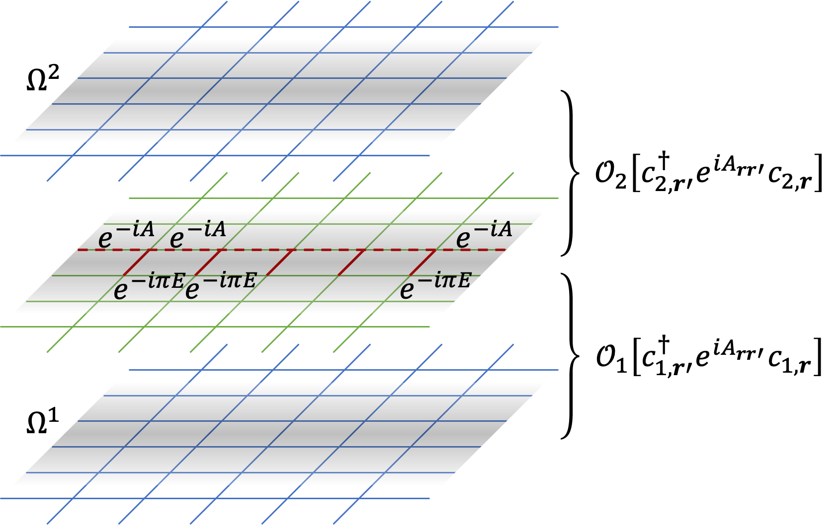
The string operator consists of three parts, , as follows (see Fig. 5):
- 1.
acts on the dynamical gauge field along the path and creates a external charge at the end of the path (and a charge at the start).
- 2.
acts on the dynamical gauge field along adjacent links to the right of and perpendicular to the path, and creates a flux at the end of the path. acts only on the gauge DOF.
- 3.
is the quasi-adiabatic responseHastings and Wen 2005 of the fermions to the flux insertion. More precisely, in each gauge field sector of the Hilbert space, we insert an external flux adiabatically, which is implemented by an -dependent evolution operator on the fermion Hilbert space. As the fermion hopping model is not exactly solvable, we do not know the exact expression for except that it is of the form
where is some gauge invariant operator generated by hopping operators . Nonetheless, properties of quasi-adiabatic evolution ensure that is local, acting only near the path (grey region in Fig. 5). A charge in and a charge in are accumulated in the process near the end of the string operator, which correspond to the fluxes of and .
We check the correctness of our string operator by computing the semion braiding phase, which we expect to be . To see this from the string operator, we break the overall commutation relation into the commutations of:
- 1.
with . This takes a charge counterclockwise around a flux, giving a phase of .
- 2.
with . This gives a phase of for the same reason.
- 3.
the product with itself. This contributes a phase which can be understood as the Berry phase obtained due to the following actions on the fermions: increasing the (background) flux in the direction by , increasing the flux in the direction by , decreasing the flux in the direction by , decreasing the flux in the direction by . In each IQH layer, the Berry phase over the entire flux parameter space is . The Berry phase over a quarter of the parameter space is therefore . As we have two IQH layers, the total phase is .
- 4.
with itself, with and with . All of these are trivial.
Summing these contributions up, we find a total braiding phase as expected. Of course, phases are defined mod , but we have been careful distinguishing e.g. from so that this argument extends naturally to general .
So far we have considered the limit, where we showed that is a string operator for the charge vector . In fact, in this limit we could write down many other different string operators for which all commute with the Hamiltonian except near the end points. For example, we could have where as before, for arbitrary and is the quasi-adiabatic response of the fermions to a flux insertion. To see why we chose the particular that satisfies the charge-flux attachment condition Eq. 17, we turn on a small , much smaller than the other couplings in the Hamiltonian and the Landau level spacing. Now if the string operator creates a flux and hence a charge in each IQH layer, then Gauss’s law (Eq. 11) implies
If , then we have an electric energy that diverges at least logarithmically. Therefore, we must choose so that . This way, when , it is possible to modify in a region near the path such that the electric energy is finite. Furthermore, since is small, the gauge field sectors that are present in the ground state can differ from the flat configuration at most by a small perturbation. Therefore, even with the new hopping coefficients , the fermions are still in a IQH state, so the flux is indeed bound with a charge in each layer. The exact expression of the new is not important, and the braiding statistic remains unchanged as long as the correct amount of external charge, fermion charge and flux are created.
A similar construction of string operators works for iCS theories. When , the string operator corresponding to standard basis vector takes the form . First, creates a external charge. Next,
creates fluxes according to the th row of , as required by Gauss’s law Eq. 15 when a small is present. The IQH layers then respond quasi-adiabatically, giving an evolution operator . The braiding statistic of and results from the commutations of with , with , and with . In particular, the commutation of with correspond to the following actions on the fermions: increasing the (background) flux in the direction by for all , increasing the flux in the direction by for all , decreasing the flux in the direction by for all , decreasing the flux in the direction by for all . A diagonal layer is coupled to only, and contributes a Berry phase of
whereas an off-diagonal layer , , is coupled to and , and contributes
The braiding phase of with is then
as can be confirmed by a straightforward calculation. Finally, we find the total braiding phase to be
as expected.
The string operators allow us to understand the profile of fractional excitations in the direction, which is determined by the fractional part of (the integral part of corresponds to local fermion and integer flux excitations). In particular, for the example of , the entries of each row of decay exponentially, which means that both and become exponentially close to the identity as we move in the direction ( is always local in the direction). Therefore, is local in the direction with an exponentially decaying tail, and the fractional excitations are localized particles. On the other hand, for , the fractional parts of the entries of do not decay. This means that the fractional excitations in the theory, if valid at all, are line excitations extended along the direction.
VI Discussion
In this paper, we established the iCS theory as a viable path to study a variety of fractonic phases. First of all, we showed in section V.1 that iCS theories with a quasi-diagonal matrix are indeed legitimate local D models by giving an explicit lattice realization for the theory. Using the method discussed in section V.2, we can further determine which iCS theories are gapped and which are gapless. Moreover, we found in section V.3 the explicit form of the string operators that create the fractional excitations in the model. From the string operators, we can learn about the nature of the fractional excitations (for example when they are localized point excitations versus when they are extensive line excitations). Based on these understandings, we found through examples an interesting variety of fractonic phenomena in iCS theories with quasi-diagonal matrices. There are 1-foliated fracton models; there are abelian type I models which do not have a foliation structure — a feature not present in previously studied models; and there are gapless theories whose nature is not clear. Some of the non-foliated gapped models have been studied previously from the perspective of coupled fractional quantum Hall layersQiu et al. 1990b; Qiu et al. 1990a; Naud et al. 2000; Naud et al. 2001, which interestingly suggests a route toward experimental realization of these particular fracton phases.
The next step would be to study iCS theories more systematically and address questions such as
- 1.
For gapped iCS theories, how can foliated theories be distinguished from non-foliated ones?
- 2.
If an iCS theory is foliated, how does one find the RG procedure that extracts 2D layers?
- 3.
How can we understand the non-foliated models, for example in terms of RG -sourcery?Swingle and McGreevy 2016
- 4.
What is the nature of the gapless models?
We hope that by addressing these questions, we can have a more complete picture of possible fractonic orders, beyond what we can learn from exactly solvable models or other frameworks.
Of course, the possibilities represented by the iCS theories are limited. The only kind of fractional excitations in these models are planons in the plane. They do not even contain fracton excitations which are completely immobile. But as we have learned from previous studies, planons play an important role in type I models. Once we have a better understanding of planons, maybe we can combine them with fractons and other sub-dimensional excitations to achieve a more complete story.
Acknowledgements.
We are indebted to inspiring discussions with Tina Zhang, Xiao-Gang Wen, Yuan-Ming Lu, Zhenghan Wang, and Kevin Slagle. We also thank Po-Shen Hsin for pointing out that a fermionic abelian topological order can always be decomposed into a bosonic abelian topological order and transparent fermions. X. M, W.S. and X.C. are supported by the National Science Foundation under award number DMR-1654340, the Simons collaboration on “Ultra-Quantum Matter” and the Institute for Quantum Information and Matter at Caltech. X.C. is also supported by the Walter Burke Institute for Theoretical Physics at Caltech. M. C. is supported by NSF CAREER (DMR-1846109) and the Alfred P. Sloan foundation. This work was supported in part by funds provided by the U.S. Department of Energy (D.O.E.) under cooperative research agreement DE-SC0009919, by the Simons Collaboration on Ultra-Quantum Matter, which is a grant from the Simons Foundation (651440, XC, ML, JM, XM, WS).References
- Nandkishore and Hermele (2019) R. M. Nandkishore and M. Hermele, Annual Review of Condensed Matter Physics 10, 295 (2019).
- Pretko et al. (2020) M. Pretko, X. Chen, and Y. You, International Journal of Modern Physics A 35, 2030003 (2020).
- Chamon (2005) C. Chamon, Phys. Rev. Lett. 94, 040402 (2005).
- Haah (2011) J. Haah, Phys. Rev. A 83, 042330 (2011).
- Vijay et al. (2016) S. Vijay, J. Haah, and L. Fu, Phys. Rev. B 94, 235157 (2016).
- Vijay et al. (2015) S. Vijay, J. Haah, and L. Fu, Phys. Rev. B 92, 235136 (2015).
- Prem et al. (2019) A. Prem, S.-J. Huang, H. Song, and M. Hermele, Physical Review X 9 (2019), 10.1103/physrevx.9.021010.
- Song et al. (2019) H. Song, A. Prem, S.-J. Huang, and M. A. Martin-Delgado, Phys. Rev. B 99, 155118 (2019).
- Ma et al. (2018) H. Ma, A. T. Schmitz, S. A. Parameswaran, M. Hermele, and R. M. Nandkishore, Phys. Rev. B 97, 125101 (2018).
- Shi and Lu (2018) B. Shi and Y.-M. Lu, Phys. Rev. B 97, 144106 (2018).
- He et al. (2018) H. He, Y. Zheng, B. A. Bernevig, and N. Regnault, Phys. Rev. B 97, 125102 (2018).
- Shirley et al. (2019a) W. Shirley, K. Slagle, and X. Chen, SciPost Physics 6 (2019a), 10.21468/scipostphys.6.1.015.
- Shirley et al. (2018) W. Shirley, K. Slagle, Z. Wang, and X. Chen, Physical Review X 8 (2018), 10.1103/physrevx.8.031051.
- Pretko (2017a) M. Pretko, Phys. Rev. B 95, 115139 (2017a).
- Pretko (2017b) M. Pretko, Phys. Rev. B 96, 035119 (2017b).
- Gromov (2019) A. Gromov, Phys. Rev. X 9, 031035 (2019).
- Seiberg and Shao (2020) N. Seiberg and S.-H. Shao, “Exotic symmetries, duality, and fractons in 3+1-dimensional quantum field theory,” (2020), arXiv:2004.00015 [cond-mat.str-el] .
- Wen (1990) X. G. Wen, International Journal of Modern Physics B 04, 239 (1990).
- Wen and Zee (1992) X. G. Wen and A. Zee, Phys. Rev. B 46, 2290 (1992).
- Shirley et al. (2019b) W. Shirley, K. Slagle, and X. Chen, “Twisted foliated fracton phases,” (2019b), arXiv:1907.09048 [cond-mat.str-el] .
- Qiu et al. (1989) X. Qiu, R. Joynt, and A. MacDonald, Physical Review B 40, 11943 (1989).
- Qiu et al. (1990a) X. Qiu, R. Joynt, and A. H. MacDonald, Phys. Rev. B 42, 1339 (1990a).
- Naud et al. (2000) J. D. Naud, L. P. Pryadko, and S. L. Sondhi, Phys. Rev. Lett. 85, 5408 (2000).
- Naud et al. (2001) J. Naud, L. P. Pryadko, and S. Sondhi, Nuclear Physics B 594, 713 (2001).
- Wall (1963) C. Wall, Topology 2, 281 (1963).
- Wang and Wang (2020) L. Wang and Z. Wang, “In and around abelian anyon models,” (2020), arXiv:2004.12048 [math.QA] .
- Levin and Fisher (2009) M. Levin and M. P. A. Fisher, Phys. Rev. B 79, 235315 (2009).
- Ma et al. (2017) H. Ma, E. Lake, X. Chen, and M. Hermele, Phys. Rev. B 95, 245126 (2017).
- Shirley et al. (2019c) W. Shirley, K. Slagle, and X. Chen, Annals of Physics 410, 167922 (2019c).
- Shirley et al. (2019d) W. Shirley, K. Slagle, and X. Chen, Physical Review B 99 (2019d), 10.1103/physrevb.99.115123.
- Wang et al. (2019) T. Wang, W. Shirley, and X. Chen, Physical Review B 100 (2019), 10.1103/physrevb.100.085127.
- Vidal (2007) G. Vidal, Phys. Rev. Lett. 99, 220405 (2007).
- Qiu et al. (1990b) X. Qiu, R. Joynt, and A. H. MacDonald, Phys. Rev. B 42, 1339 (1990b).
- (34) The integers 1, 4, 11, 29, etc. form a sequence known as the Lucas numbers.
- Kitaev (2006) A. Kitaev, Annals of Physics 321, 2 (2006), january Special Issue.
- Kalmeyer and Laughlin (1987) V. Kalmeyer and R. B. Laughlin, Phys. Rev. Lett. 59, 2095 (1987).
- Hastings and Wen (2005) M. B. Hastings and X.-G. Wen, Phys. Rev. B 72, 045141 (2005).
- Swingle and McGreevy (2016) B. Swingle and J. McGreevy, Phys. Rev. B 93, 045127 (2016).
Appendix A A class of foliated iCS theories
The twisted 1-foliated fractonic order Eq. 3 can be generalized to a class of foliated iCS theories, with matrix parameterized by integers and :
where and takes value in . This can be obtained by boson condensation in a stack of twisted gauge theories, in a way that naturally generalizes the procedure in Ref. Shirley et al. 2019b. To see the foliation structure, take
where the action of outside this block is the identity. We find that decouples into and two copies of twisted gauge theories described by
The fusion group when and are coprime is
When and are not coprime, we can factor out from and analyze similarly.
Appendix B A class of non-foliated iCS theories
In this appendix, we generalize and to a class of non-foliated iCS theories described by
, and derive various quantities regarding . We first consider a different matrix
which is obtained from by removing the entries in the top-right and bottom-left corners. We will compute , which will be useful when we compute and later in this appendix. To do this, we need to take exactly one entry from each row and one from each column. If entry is used from the first row, then the rest is just . Otherwise, entry must be used, and therefore so must be entry , and the rest is . We thus obtain the recurrence relation
| (18) |
Solving this with the initial conditions and , we find
where .
Now we compute . Depending on whether entries and are used, we can write
| (19) |
where the first term uses neither of the entries and , the second and third terms uses exacly one, and the third term uses both. Further simplification then gives Eq. 7. Incidentally, the recurrence relation Eq. 18 has characteristic polynomial
and Eq. 19 implies that satisfies a third order recurrence relation whose characteristic polynomial has a third root in addition to those of . Thus
and satisfies a third order recurrence relation
The fusion group for is of the form
where depends on and as follows:
- •
If is odd, then . A choice of generators is for and for .
- •
If is even and is odd, then . A choice of generators is for and for .
- •
If is even and is even, then . A choice of generators is for and for .
Finally, after manipulating determinants like we did when computing and , we find
where . Eq. 8 then follows by plugging in .
Appendix C Determining matrix from statistics
In this appendix, we answer the following question: given an abelian topological order with its anyon fusion and statistics specified, how does one construct a corresponding CS theory?
More precisely, the setup of the problem consists of:
- 1.
A finite abelian fusion group . We write the fusion product of and as instead of the usual .
- 2.
A symmetric bilinear function which gives the braiding statistic between anyons and . Bilinearity means that and similarly for the second argument.
- 3.
A function which is related to via
and determines topological spins by . With respect to a minimal generating set of , we can write as a matrix where and if .
Note that does not determine even though the converse is true. Indeed, , but itself is defined mod 2. This is the minus sign ambiguity in determining exchange statistic from braiding statistic. We focus on bosonic topological orders and assume modularity of the topological -matrix, which in our language means that is non-degenerate in the sense that if for all , then . We comment on fermionic topological orders in Section C.4.
Our goal is to find a matrix that produces the specified above. Naively, this is achieved by inverting the matrix . For example, the toric code has
so we can take
However, is not an integer matrix for a generic . For example, the three-fermion theory has and
but is not an integer matrix. Instead, we need to “enlarge” to by adding transparent bosons (i.e. bosons that braid trivially with everything) to the bottom right corner:
To obtain an enlargement algorithm that works for arbitrary , we follow the strategy by Wall Wall 1963; Wang and Wang 2020: first we present a structure theorem for , which classifies all irreducible building blocks of and gives an algorithm for decomposing into these blocks. Then we write down an enlargement for each irreducible block.
C.1 Structure theorem
Given and subgroups , of , we say that is the orthogonal direct product of and if and for all , . We have the following structure theorem:
Theorem C.1
If is non-degenerate, then can be written as an orthogonal direct product such that is in one of the following irreducible classes labelled by letters through :
- 1.
, and .
- 2.
, prime, and where is coprime with and is a quadratic residue mod . ( is a quadratic residue mod if for some .) Different choices of lead to the same up to change of generator.
- 3.
, and .
- 4.
, prime, and where is coprime with and is not a quadratic residue mod . Different choices of lead to the same up to change of generator.
- 5.
, , and .
- 6.
, , and .
- 7.
, and .
- 8.
, and .
The above decomposition is not unique, e.g. and . The toric code is in class and the three-fermion theory is in .
Before we describe how the decomposition in Theorem C.1 can be performed, we state the following useful lemma:
Lemma C.2
Let be non-degenerate, a subgroup of such that is non-degenerate. Then is the orthogonal direct product of and its orthogonal complement , and is also non-degenerate.
We perform the decomposition in Theorem C.1 using the following three steps:
- •
Step 1. We can uniquely decompose
(20) where is the unique Sylow -subgroup of . This product is always orthogonal.
- •
Step 2. Now we replace for fixed . Let be the exponent of , i.e. the least common multiple of the orders of all elements in . Write as a (non-orthogonal) direct product of a homogeneous subgroup of exponent ,i.e. for some , and another subgroup of smaller exponent. One can show that is non-degenerate. Lemma C.2 then gives which is an orthogonal direct product, and has exponent smaller than . Proceeding in this way, we can decompose into an orthogonal direct product of homogeneous subgroups.
- •
Step 3. Replace again by a homogeneous group of exponent , . We look for such that is coprime with . Such need not exist when , but when it exists it is often easy to spot by inspection. However, for generality we present a more organized method (readers may skip this part and jump to Cases 3.1 & 3.2 below). Consider the subgroup of , where is the order of , and write for the coset containing in . Define a new bilinear function by
Now we look for some such that is coprime with . If , such always exists, and although we may still need an exhaustive search, this search is easier since has a smaller size than . If , such exists if and only if the th diagonal element of is nonzero for some , in which case the generating element satisfies our requirement. Our next step depends on whether or not such was found:
Case 3.1. We found some with coprime with . Then is non-degenerate, where is an arbitrary coset representative and is the subgroup of generated by . Lemma C.2 then gives , and we go back to Step 3.
Case 3.2 (occurs only if ). for all . Pick some of order , e.g. a generating element . One can show that there exists (not necessarily unique) such that . Let and be arbitrary coset representatives. Then is non-degenerate, and or . Again we apply Lemma C.2 and then go back to Step 3.
Recursive application of the above steps leads to full decomposition of .
C.2 Enlargement algorithm
Now we describe how to enlarge the matrix to such that is an integer matrix with even diagonal, so that describes a bosonic CS theory. Using Theorem C.1, we assume without loss of generality that is in one of the classes through .
- 1.
, or . No enlargement is needed.
- 2.
or with . Write for some . Then there exist even and odd such that and . Next, choose even such that is the closest even multiple of to , and write . Continuing this algorithm, we obtain
where is always the closest even multiple of to . Then we take
The algorithm we employed to produce is a variation of the Euclidean algorithm.
- 3.
or . In this case the Euclidean algorithm still works, but we need to take odd and even.
- 4.
. We take
(21)
C.3 Example
We demonstrate the procedures in the previous sections with a coined example ,
Since is already homogeneous, we jump straight to Step 3. First we spot that has additive order 8 mod 1, so is non-degenerate. We therefore compute , where , , , . With respect to these generators, we have
Since all diagonal entries of have denominators at most 4, we turn to Case 3.2 and pick any generator, say . The equation has a solution . Then we work out
With respect to the generators , we have
where is the direct sum of matrices on the direct product group. Picking appropriate generators , we can put into a standard form
To summarize,
| (22) |
with respect to the generators
However, this decomposition is not unique; with respect to some other generators, we also have
Next, we enlarge each summand in Eq. 22. To enlarge the , we apply the Euclidean algorithm:
which gives
The does not need enlargement, and the can be enlarged to Eq. 21.
This completes our example. The total inverse matrix is
and the total matrix is
C.4 Fermionic case
Finally, we consider fermionic topological orders. Now a local fermion excitation is a superselection sector that braids trivially with everything, i.e. a transparent fermion, so we need to modify our non-degeneracy assupmtion. We assume that is weakly non-degenerate in the sense that if for all and , then .
Suppose that is a transparent fermion. Since , in the decomposition Eq. 20 we must have . Suppose for some and . Then
so must be odd. But , so and hence . Thus we have proved that is not a non-trivial multiple of any , so can be decomposed into an orthogonal direct product of and . Continuing this process, we end up with where each is generated by a transparent fermion and is non-degenerate. The bosonic result can then be applied to .
As an example, consider the fractional quantum Hall effect. Treated as a bosonic theory, the fusions group is , whose generator we call , and . This theory is only weakly non-degenerate, with a transparent fermion. Following the above recipe, we decompose . Now is non-degenerate, where
We can then use the Euclidean algorithm to enlarge it to
Putting the transparent fermion back, we get a matrix which can be mapped through a general linear transformation as follows:
where
This shows the equivalence of our result with the standard matrix (3) for the fractional quantum Hall state.