PLS for V2I Communications Using Friendly Jammer and Double kappa-mu Shadowed Fading Thanks: 

Wireless vehicular network (WVN) has been exponentially evolving by taking advantage of sophisticated technologies such as artificial intelligence (AI) [1], machine learning [2], Millimeter Wave (mmWave) [3, 4, 5, 6, 7], and 5G [8, 9, 10], etc. It offers a variety of advanced features like real-time alerting messages [11], cloud services [12, 13], etc. However, as any communication network, WVN is subject to many challenges, especially the security issue which is a peer parameter that guarantees a certain acceptable quality of services (QoS).
Several research papers discussed the security challenges and proposed a variety of solutions from different OSI (Open Systems Interconnection model) layers perspective [14, 15]. Regarding the physical layer security (PLS), it has been proven that securing the communication at this level is an efficient scheme to deal with passive threats like the eavesdropping attacks. In this kind of menace, the malicious network entity is able to listen to a private communication by intercepting the transmitted signal and revealing the confidential information.^††footnotetext: This work was supported in part by the U.S. National Science Foundation (NSF) under the grant CNS-1650831. What makes the eavesdropping attacks very critical is the fact that it is difficult to be detected by the victims since it could be processed without leaving any traces. To deal with this security dilemma, some related works proposed the use of artificial noise (AN) where the transmitter perturbs the attacker channel by sending a dedicated signal [16, 17]. This signal is generated orthogonally to the main link between the legitimate entities so that it will affect only the eavesdropper link. Other papers studied the employment of a friendly jammer (J) which has the responsibility of jamming the eavesdroppers’ channels instead of the transmitter [18, 19].
In general, by employing a jammer $J$, as a third network entity, could be more efficient in the case of multiple eavesdroppers attacks. In other words, if the network is subject to several attacks, it is better to have a jammer node to deal with all the attackers rather than each communicating node deals with all the attackers by itself (it will be very expensive in terms of power if each transmitter will dedicate a fraction of its power to jam all the eavesdroppers’ channels).

In our paper, we are focusing on using the friendly jammer to protect V2I communications. As a channel fading, we adopt the Double Shadowed $\kappa$-$\mu$ Fading Model, noted by $\mathcal{D}(\cdot)$, recently presented in [20], which is more general and covers wide ranges of fading such as double shadowed Rice, Rician shadowed, Nakagami-q, Nakagami-m, Rayleigh, one-sided Gaussian, etc. We highlight our contributions as follows:

1. $\bullet$

   We propose the use of friendly jammer $J$ in V2I communications under an eavesdropping attack scenario.

2. $\bullet$

   We adopt the new channel model $\mathcal{D}(\cdot)$.

3. $\bullet$

   We derive a closed form expression for the ergodic capacity at the receiver under $\mathcal{D}(\cdot)$ model.

4. $\bullet$

   We derive a closed form expression for cumulative distribution function (CDF) of the signal-to-interference-plus-noise-ratio (SINR) and the ergodic capacity at the eavesdropper while considering Nakagami-m as special case of $\mathcal{D}(\cdot)$.

5. $\bullet$

   We examine the impact of the blockage density at the receiver by adopting the special case model Rician shadowed.

The paper is constructed as follows: Section II introduces the system model. Section III studies the outage probability while Section IV examines the ergodic capacity and the secrecy capacity. Then, Section V evaluates the performance of the security approach based on numerical results. Finally, we outline our conclusion in Section VI.

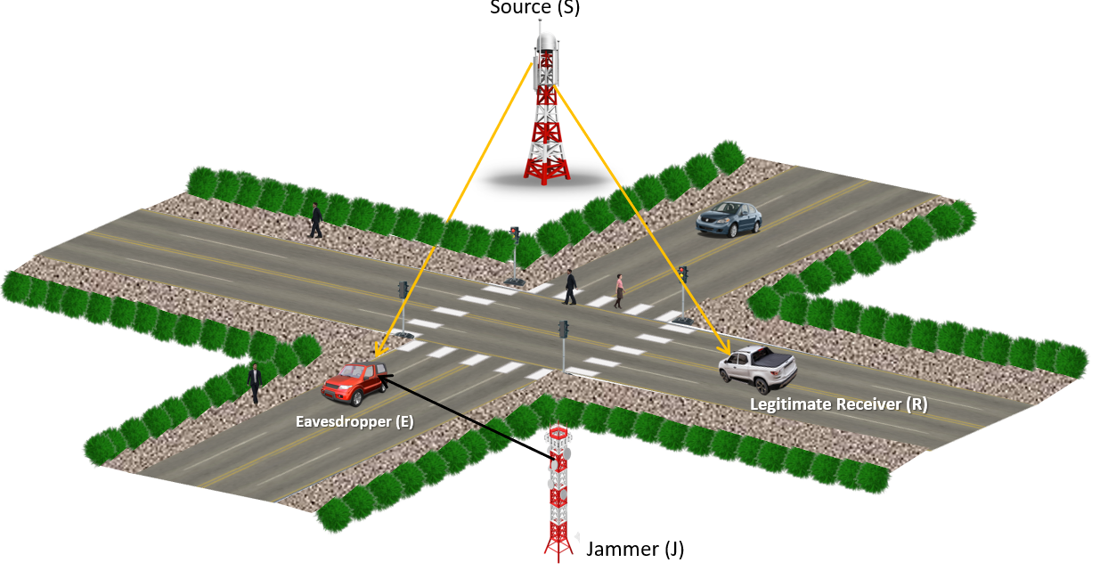
In V2I communications, base stations (BSs) and vehicles should be able to exchange information and data securely. However, the transmitted signals may be subject to an intended overhearing where an eavesdropper intercepts the signal and reveals the secret messages. In Fig. 1, we have a typical model where the attacker E is listening to the communication between the source $S$ (the base station) and the legitimate receiver $R$. In this case, $J$ tends to protect the network by sending AN to the attacker $E$, while $R$ is immune since the AN is orthogonal to its channel.

The received signal at R and E are respectively:

where the channel model parameters are defined in Table I.

As we can deduce from Eq. (1), $\sum_{k=1}^{K}h_{{}_{J,R}}x_{{}_{J}}=0$, which means that the jamming signal will only affect the attacker while conserving the same signal at the legitimate receiver.
The received SNR and SINR at $R$ and $E$, respectively, are

where $\gamma_{{}_{R;n}}$ $\sim$ $\mathcal{D}(\cdot)$ and $\gamma{{}_{{}_{I;n}}}$ $\sim$ $\mathcal{D}(\cdot)$ are, respectively, the SNRs corresponding to the confidential signal received at $R$ and $E$ via the $n$-th antenna, while $\gamma{{}_{{}_{J;k}}}$ $\sim$ $\mathcal{D}(\cdot)$ is the SNR due to the jamming signal sent by $J$ at $E$ via the $k$-th antenna. The general probability density function (PDF) and CDF of the random variable (RV) $\gamma_{{}_{l}}$, where $l\in\{(I;n),(J;k),(R;n)\}$, are respectively

where ${}_{2}F_{1}(\cdot,\cdot;\cdot;.)$ represents the Hypergeometric function, $B(\cdot,\cdot)$ denotes the Beta function, $\tau=\frac{-T_{{}_{l}}\gamma}{\overline{\gamma}(s_{{}_{l}}-1)}$ and $(x)_{i}=\frac{\Gamma(x+i)}{\Gamma(x)}$ is the the Pochhammer symbol. For the sake of organization, the parameters on which depends the distribution of $\gamma_{{}_{l}}$, are presented in Table. II.

To analyze the outage probability at $R$, we have to refer to the corresponding CDF. We know that $\gamma_{{}_{R;n}}$ $\sim$ $\mathcal{D}(\cdot)$, hence its CDF is given by Eq. (6). However, the closed-form expression of the CDF corresponding of $\sum_{n=1}^{N}\gamma_{{}_{R;n}}$ is not tractable. Therefore, we are assuming that N = 1, which make the outage probability of $\gamma_{{}_{R}}$ represented by Eq. (6). At this stage, we are referring to the special fading case Rician shadowed under the following substitutions: $c_{R}\rightarrow\infty$ and $\mu=1$ [20]. Therefore, the CDF is expressed as follows [21]

where $\gamma(\cdot,\cdot)$ is the Incomplete Gamma function, $\Xi$ is the average power of the line of sight (LOS) component, $2\sigma^{2}$ is the average power of the scatter component, $m$ is fading figure which represents the fading severity. Therefore, the outage related to the density of shadowing, $F_{\gamma_{{}_{SD}}}$ could be presented by

where $F_{\gamma_{{}_{SD}}}^{{}_{los}}(\gamma)$ and $F_{\gamma_{{}_{SD}}}^{{}_{nlos}}(\gamma)$ are the CDFs of the SNR evaluated when the link is LOS, and non-line-of-side (NLOS), respectively.

It is complex to derive a closed-form expression of the CDF at the eavesdropper $E$. However, we can take advantage of the $\mathcal{D}(\cdot)$ generality by considering special channel model cases by manipulating its parameters. We suggest that $h_{S,E}$ and $h_{J,E}$ follow Nakagami-m distribution by fixing $c_{{}_{R}}=s_{{}_{R}}=\infty$, $\mu_{{}_{I}}=1$ and $\kappa_{{}_{I}}=m$[20]. Hence, $\gamma_{{}_{I;n}}$ and $\gamma_{{}_{J;k}}$ (see Eq. (4) ) are described by Gamma distribution ($\gamma_{{}_{I;n}}\sim\textit{{G}}(\nu_{{}_{I,n}},\beta_{{}_{I,n}})$ and $\gamma_{{}_{J;k}}\sim\textit{{G}}(\nu_{{}_{J,k}},\beta_{{}_{J,k}})$ ) , which has the following PDF and CDF

where $d\in\{(I;n),(J;k)\}$, $\beta_{{}_{h}}$ and $\nu{{}_{h}}$ are, respectively, the scale and the shape parameters. Each antenna of the BS has the same distance from the attacker because the antennas are collocated. Therefore the parameter $\beta_{{}_{I,n}}$ is the same for all antennas $n\in{1,...,N}$ ($\beta{{}_{I}}$=$\beta_{{}_{I;n}}$) since $\beta_{{}_{S,E;n}}=\frac{P_{{}_{S}}r_{{}_{S,E;n}}^{-\delta}}{\sigma_{w_{{}_{E}}}^{2}}$. We assume that all N links have the same scale parameter, which means $\nu{{}_{I}}$=$\sum_{n=1}^{N}\nu_{{}_{I;n}}$. Therefore $\sum_{n=1}^{N}\gamma_{{}_{I;n}}=\gamma_{{}_{I}}$ $\sim$ $\textit{{G}}(\nu_{{}_{I}},\beta_{{}_{I}})$. The same analogy applied to the signal issued by the jammer where $\sum_{k=1}^{K}\gamma_{{}_{J;k}}=\gamma_{{}_{J}}$ $\sim$ $\textit{{G}}(\nu_{{}_{J}},\beta_{{}_{J}})$. For the sake of mathematical simplicity, we assume that $\nu_{{}_{h}}$ is a positive integer. Accordingly, the CDF has the subsequent series expansion as:

Before deriving the CDF at $E$ following the aforementioned special cases, we should mention that we verified and proved obtaining Nakagami-m distribution by using the general PDF of the envelope corresponding to $\mathcal{D}(\cdot)$ and substituting the appropriate parameters (Please refer to the Appendix).
By referring to Eq. (4), Eq. (9), and Eq. (11), the CDF at the attacker can be derived using the following expression

where $\Omega=q+\nu_{{}_{J}}$.
Then, by referring to [[22], Eq (3.351.3)], we obtain

By referring to Eqs. (5, 6, and 14), the ergodic capacity at the legitimate receiver can be expressed by:

To find a closed form of the aforementioned expression, we rewrite the following expressions as follow [23]

where $G^{m,n}_{p,q}\left(\begin{matrix}-|(\cdot,\cdot)\end{matrix}\right)$ is the Meijer G-Function, $\Phi=(s_{{}_{R}}-1)\overline{\gamma}_{{}_{L}},\alpha=\mu_{{}_{R}}+i,$ and $\eta=i+s_{{}_{R}}+\mu_{{}_{R}}.$
Then, by substituting Eq. (17) and Eq. (18) in Eq. (16) and by referring to the [[24], 07.34.21.0011.01], we obtain:

Using Eq. (13) and Eq. (14), we can write the ergodic capacity as follows

To facilitate the integral calculation, we can perform the following transformation into Fox-H function

Then, we substitute Eq. (21) and Eq. (22) in Eq. (20) and we compute the integral [25]. Hence, we obtain

where $H_{m_{1},n_{1};m_{2},n_{2};m_{3},n_{3}}^{p_{1},q_{1};p_{2},q_{2};p_{3},q_{3}}(-|(\cdot,\cdot))$ is the bivariate Fox H-function [26, 27]. Therefore, by substituting Eq. (19) and Eq. (23) into Eq. (15), we obtain the average secrecy capacity as given on the top of the next page.

References

- [1] W. Tong, A. Hussain, W. X. Bo, and S. Maharjan, “Artificial intelligence for vehicle-to-everything: A survey,” IEEE Access, vol. 7, pp. 10 823–10 843, 2019.
- [2] S. S. Doddalinganavar, P. V. Tergundi, and R. S. Patil, “Survey on deep reinforcement learning protocol in vanet,” in 2019 1st International Conference on Advances in Information Technology (ICAIT), 2019, pp. 81–86.
- [3] E. Balti and B. K. Johnson, “Tractable approach to mmwaves cellular analysis with fso backhauling under feedback delay and hardware limitations,” IEEE Transactions on Wireless Communications, vol. 19, no. 1, pp. 410–422, 2020.
- [4] E. Balti, M. Guizani, B. Hamdaoui, and B. Khalfi, “Aggregate hardware impairments over mixed rf/fso relaying systems with outdated csi,” IEEE Transactions on Communications, vol. 66, no. 3, pp. 1110–1123, 2018.
- [5] Y. Yang, Z. Gao, Y. Ma, B. Cao, and D. He, “Machine learning enabling analog beam selection for concurrent transmissions in millimeter-wave v2v communications,” IEEE Transactions on Vehicular Technology, vol. 69, no. 8, pp. 9185–9189, 2020.
- [6] E. Balti, M. Guizani, and B. Hamdaoui, “Hybrid rayleigh and double-weibull over impaired rf/fso system with outdated csi,” in 2017 IEEE International Conference on Communications (ICC), 2017, pp. 1–6.
- [7] E. Balti, N. Mensi, and S. Yan, “A modified zero-forcing max-power design for hybrid beamforming full-duplex systems,” 2020.
- [8] A. Hussein, I. H. Elhajj, A. Chehab, and A. Kayssi, “Sdn vanets in 5g: An architecture for resilient security services,” in 2017 Fourth International Conference on Software Defined Systems (SDS), 2017, pp. 67–74.
- [9] E. Balti, M.Guizani, B. Hamdaoui, and Y. Maalej, “Partial relay selection for hybrid rf/fso systems with hardware impairments,” in 2016 IEEE Global Communications Conference (GLOBECOM), 2016, pp. 1–6.
- [10] E. Balti, M. Guizani, B. Hamdaoui, and B. Khalfi, “Mixed rf/fso relaying systems with hardware impairments,” in GLOBECOM 2017 - 2017 IEEE Global Communications Conference, 2017, pp. 1–6.
- [11] A. H. Khosroshahi, P. Keshavarzi, Z. D. KoozehKanani, and J. Sobhi, “Acquiring real time traffic information using vanet and dynamic route guidance,” in 2011 IEEE 2nd International Conference on Computing, Control and Industrial Engineering, vol. 1, 2011, pp. 9–13.
- [12] N. Mensi, M. Guizani, and A. Makhlouf, “Study of vehicular cloud during traffic congestion,” in 2016 4th International Conference on Control Engineering Information Technology (CEIT), 2016, pp. 1–6.
- [13] Y. Maalej, A. Abderrahim, M. Guizani, B. Hamdaoui, and E. Balti, “Advanced activity-aware multi-channel operations1609.4 in vanets for vehicular clouds,” in 2016 IEEE Global Communications Conference (GLOBECOM), 2016, pp. 1–6.
- [14] Deeksha, A. Kumar, and M. Bansal, “A review on vanet security attacks and their countermeasure,” in 2017 4th International Conference on Signal Processing, Computing and Control (ISPCC), 2017, pp. 580–585.
- [15] N. Mensi, A. Makhlouf, and M. Guizani, “Incentives for safe driving in vanet,” in 2016 4th International Conference on Control Engineering Information Technology (CEIT), 2016, pp. 1–6.
- [16] H. Wang, T. Zheng, and X. Xia, “Secure miso wiretap channels with multiantenna passive eavesdropper: Artificial noise vs. artificial fast fading,” IEEE Transactions on Wireless Communications, vol. 14, no. 1, pp. 94–106, 2015.
- [17] O. Cepheli and G. K. Kurt, “Analysis on the effects of artificial noise on physical layer security,” in 2013 21st Signal Processing and Communications Applications Conference (SIU), 2013, pp. 1–4.
- [18] V. Bankey and P. K. Upadhyay, “Improving secrecy performance of land mobile satellite systems via a uav friendly jammer,” in 2020 IEEE 17th Annual Consumer Communications Networking Conference (CCNC), 2020, pp. 1–4.
- [19] B. Li, Y. Zou, J. Zhou, F. Wang, W. Cao, and Y. Yao, “Secrecy outage probability analysis of friendly jammer selection aided multiuser scheduling for wireless networks,” IEEE Transactions on Communications, vol. 67, no. 5, pp. 3482–3495, 2019.
- [20] N. Simmons, C. R. Nogueira da Silva, S. L. Cotton, P. C. Sofotasios, S. Ki Yoo, and M. D. Yacoub, “The double shadowed fading model,” in 2019 International Conference on Wireless and Mobile Computing, Networking and Communications (WiMob), 2019, pp. 1–6.
- [21] H. Stefanovic, V. Stefanovic, A. Cvetkovic, J. Anastasov, and D. Stefanovic, “Some statistical characteristics of a new shadowed rician fading channel model,” in 2008 The Fourth International Conference on Wireless and Mobile Communications, 2008, pp. 235–240.
- [22] I. S. Gradshteyn and I. M. Ryzhik, Table of integrals, series, and products, 7th ed. The Netherlands:Academic, 2007.
- [23] E. Balti and M. Guizani, “Mixed rf/fso cooperative relaying systems with co-channel interference,” IEEE Transactions on Communications, vol. 66, no. 9, pp. 4014–4027, 2018.
- [24] W. R. Inc., “Mathematica, Version 12.1,” champaign, IL, 2020. [Online]. Available: https://www.wolfram.com/mathematica
- [25] P. K. Mittal and K. C. Gupta, “An integral involving generalized function of two variables,” Proceedings of the Indian Academy of Sciences - Section A, vol. 75, no. 3, pp. 117–123, 1972.
- [26] E. Balti and M. Guizani, “Impact of non-linear high-power amplifiers on cooperative relaying systems,” IEEE Transactions on Communications, vol. 65, no. 10, pp. 4163–4175, 2017.
- [27] E. Balti, “Analysis of hybrid free space optics and radio frequency cooperative relaying systems,” Master’s thesis, 2018.
- [28] A. Abdi, W. C. Lau, M. . Alouini, and M. Kaveh, “A new simple model for land mobile satellite channels: first- and second-order statistics,” IEEE Transactions on Wireless Communications, vol. 2, no. 3, pp. 519–528, 2003.