Squashing activation functions in benchmark tests: towards eXplainable Artificial Intelligence using continuous-valued logic
Abstract
Over the past few years, deep neural networks have shown excellent results in multiple tasks, however, there is still an increasing need to address the problem of interpretability to improve model transparency, performance, and safety. Achieving eXplainable Artificial Intelligence (XAI) by combining neural networks with continuous logic and multi-criteria decision-making tools is one of the most promising ways to approach this problem: by this combination, the black-box nature of neural models can be reduced. The continuous logic-based neural model uses so-called Squashing activation functions, a parametric family of functions that satisfy natural invariance requirements and contain rectified linear units as a particular case. This work demonstrates the first benchmark tests that measure the performance of Squashing functions in neural networks. Three experiments were carried out to examine their usability and a comparison with the most popular activation functions was made for five different network types. The performance was determined by measuring the accuracy, loss and time per epoch. These experiments and the conducted benchmarks have proven that the use of Squashing functions is possible and similar in performance to conventional activation functions. Moreover, a further experiment was conducted by implementing nilpotent logical gates to demonstrate how simple classification tasks can be solved successfully and with high performance. The results indicate that due to the embedded nilpotent logical operators and the differentiability of the Squashing function, it is possible to solve classification problems, where other commonly used activation functions fail.
Keywords:
XAI , neural networks , Squashing function , continuous logic , fuzzy logic1 Introduction
While AI techniques, especially deep learning techniques, are revolutionizing the business and technology world, there is an increasing need to address the problem of interpretability and to improve model transparency, performance, and safety: a problem that is of vital importance to all our research community. This challenge is closely related to the fact that although deep neural networks have achieved impressive experimental results, especially in image classification, they have shown to be surprisingly unstable when it comes to adversarial perturbations: minimal changes to the input image may cause the network to misclassify it. Moreover, although machine learning algorithms are capable of learning from a set of data and of producing a model that can be used to solve different problems, the values of the accuracy or the prediction error are not enough, since these numbers only provide an incomplete description of most real-world problems. The interpretability of a machine learning model gives insight on its internal functionality to explain the reasons why it suggests making certain decisions. In low-risk environments, such as film recommendation, only the predictive performance of the model counts. However, in high-risk environments, such as the health care or the insurance sector, it is important to be able to explain why a decision was made. In this case, we need to have some reasonable explanations behind our decisions to be more convincing and also to avoid lawsuits claiming race-based, gender-based, or age-based bias [1]. Understandability means that we are able to describe the computations by using words from natural human language. One of the main challenges here is that natural language is often imprecise (fuzzy), making it difficult to find the relation between imprecise words and mathematical algorithms. This experience led to the design on fuzzy logic by Zadeh; see, e.g., [2, 3, 4, 5, 6]. The reason, why human-led control often leads to much better results than even the optimal automatic control is that humans use additional knowledge.
The basic idea of continuous logic is the replacement of the space of truth values by a compact interval such as . This means that the inputs and the outputs of the extended logical gates are real numbers of the unit interval, representing truth values of inequalities. Quantifiers and are replaced by and , and logical connectives are continuous functions. Based on this idea, human thinking and natural language can be modeled in a more sophisticated way. Among other families of fuzzy logics, nilpotent fuzzy logic is beneficial from several perspectives. The fulfillment of the law of contradiction and the excluded middle, and the coincidence of the residual and the S-implication [7, 8] make the application of nilpotent operators in logical systems promising. In [9, 10, 11, 12, 13, 14], an abundant asset of operators was examined thoroughly: in [10], negations, conjunctions and disjunctions, in [11] implications, and in [12] equivalence operators. In [13], the aggregative operators were studied and a parametric form of a general operator was given by using a shifting transformation of the generator function. Varying the parameters, nilpotent conjunctive, disjunctive, aggregative (where a high input can compensate for a lower one) and negation operators can all be obtained. It was also demonstrated how the nilpotent generated operator can be applied for preference modeling. Moreover, as shown in [14], membership functions, which play a substantial role in the overall performance of fuzzy representation, can also be defined using a generator function.
In [15, 16], the authors introduced an idea of achieving eXplainable Artificial Intelligence (XAI) by combining neural networks with nilpotent fuzzy logic as a promising way to approach the problem: by this combination, the black-box nature of neural models can be reduced, and the neural network-based models can become more interpretable, transparent, and safe. In [15], the authors showed that in the field of continuous logic, nilpotent logical systems are the most suitable for neural computation. To achieve the transparency using logical operators, it is desirable to chose an activation function that fits the theoretical background the best. In the formulae of the nilpotent operators, the cutting function (Heaviside or binary threshold function) plays a crucial role. Although piecewise linear functions are easy to handle, there are areas where the parameters are learned by a gradient-based optimization method. In this case, the lack of continuous derivatives makes the application impossible. To address this problem, a continuously differentiable approximation of the cutting function, the Squashing function, introduced in [17], was used in the nilpotent neural model [15], [16]. In [18], the authors explain the empirical success of Squashing functions by showing that the formulas describing this family (that contain rectified linear units as a particular case) follow from natural invariance requirements.
This study provides the first benchmark tests that measure the performance of the Squashing functions in neural networks and also demonstrates the first steps towards the implementation of nilpotent logical gates. The article is organized as follows. After recalling the most important preliminaries in Section 2, Section 3 provides three experiments to demonstrate the usability of squasing activation functions together with a comparison with the most popular activation functions for five different network types. The performance of these functions was determined by measuring accuracy, loss and time per epoch. These experiments and the conducted benchmarks have proven that the use of the Squashing function is possible and similar in performance to the conventional activation functions. In Section 4, a further experiment was conducted by implementing nilpotent logical gates to demonstrate how simple classification tasks can be performed successfully and with high performance. Due to their low complexity, these networks are easy to interpret and analyze. The results indicate that due to nilpotent logical operators and the differentiability of the Squashing function, it is possible to solve classification problems, where other commonly used activation functions fail. Finally, in Section 5, the main results are summarized.
2 Preliminaries
First, we recall some important preliminaries regarding nilpotent logical systems and Squashing functions.
2.1 Nilpotent logical systems
As mentioned in the Introduction, in the field of continuous logic, nilpotent logical systems are the most suitable for neural computation. For more details about nilpotent systems see [9, 10, 11, 12, 13, 14, 15]. In [13], the authors examined a general parametric operator, , of nilpotent systems.
Definition 1.
[13] Let be an increasing bijection, , and where and let us define the general operator by
| (1) |
Remark 1.
Note that the general operator for is conjunctive, for it is disjunctive and for it is self-dual.
As a benefit of using this general operator, a conjunction, a disjunction and an aggregative operator differ only in one parameter of the general operator in Equation (1). Additionally, the parameter has the semantic meaning of the level of expectation: maximal for the conjunction, neutral for the aggregation, and minimal for the disjunction.
| for | Notation | |||||
| LOGICAL OPERATORS | ||||||
| disjunction | ||||||
| conjunction | ||||||
| implication | ||||||
| MULTI-CRITERIA DECISION TOOLS | ||||||
| arithmetic mean | ||||||
| preference | ||||||
| aggregative operator | ||||||
Next, let us recall the weighted form of the general operator:
Definition 2.
[13] Let an increasing bijection with where The weighted general operator is defined by
| (2) |
Note that if the weight vector is normalized; i.e. for
| (3) |
For future application, we introduce a threshold-based operator in the following way.
Definition 3.
[13] Let , and let be a strictly increasing bijection. Let us define the threshold-based nilpotent operator by
| (4) |
where
| (5) |
Remark 2.
Note that the Equation in (4) describes the perceptron model in neural computation. Here, the parameters all have semantic meanings as importance (weights), decision level and level of expectancy. Table 1 shows how the logical operators and some multi-criteria decision tools, like the preference operator, can be implemented in neural models.
The most commonly used operators for and for special values of and , also for , are listed in Table 1.
2.2 Squashing Function as a differentiable parametric approximation of the Heaviside Function
As highlighted in the Introduction, in the formulae of the nilpotent operators, the cutting function plays a critical role (see Table 1). To address the problem of the lack of differentiability, the following approximation, the so-called Squashing function (introduced in [17]) was used in the nilpotent neural model [15], [16] .
Definition 4.
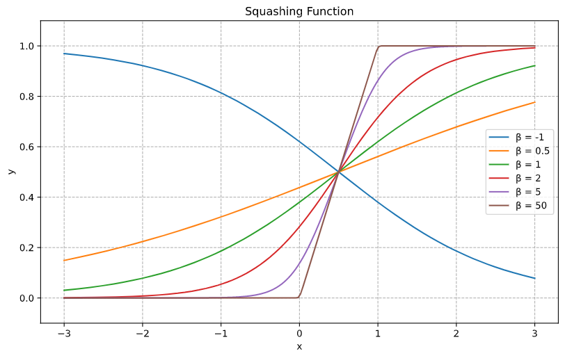
The Squashing function given in Definition 4 is a continuously differentiable approximation of the generalized cutting function by means of sigmoid functions (see Figure 1). By increasing the value of , the Squashing function approaches the generalized cutting function. In other words, drives the accuracy of the approximation, while the parameters and determine the center and width. The error of the approximation can be upper bounded by , which means that by increasing the parameter , the error decreases by the same order of magnitude. The derivatives of the Squashing function are easy to calculate and can be expressed by sigmoid functions and itself:
| (8) |
In [18], it is shown that the formulas describing the squashing functions follow from natural symmetry requirements and contain linear units as a particular case.
3 Implementation and benchmark tests
This section describes the exact implementation of the Squashing function in the PyTorch framework (GitHub Repository [19]). To verify this implementation, three experiments were conducted. First, the basics of these experiments are introduced and the datasets are presented. The results obtained by using Squashing functions in different benchmark tasks, including tests in different neural network architectures and a comparison with commonly used activation functions, indicate that the Squashing function is capable of performing similarly to other popular activation functions. As a starting point, in Section 3.1, the behavior of the Squashing function with , , and learnable parameter is investigated.
3.1 Testing of the Squashing Function
The test phase is divided into three experiments. The goal is to see if the Squashing function could solve simple classification problems. Each of these experiments consisted of classifying a set of data that are distributed in different shapes. The dataset is composed of two balanced classes, each containing 250 points. In the first experiment, two point clouds are to be separated by a straight line. In the second experiment, these point clouds are arranged in circular configurations as seen in Figure 2b. In the last experiment, the point sets formed two intertwined spirals.

3.1.1 Experiment 1: Classification of Gaussian Data
The task of the first experiment is solved with a one-layer feedforward network. The model architecture shown in Table 2 uses a fully-connected layer with two input and two output features.
| Type of layer | Number of input features | Number of output features |
|---|---|---|
| Fully-connected | 2 | 2 |
As a cost function cross-entropy function is applied, while the Adam optimization algorithm is utilized for the optimization procedure. The training process takes 10 epochs with a learning rate of
Figure 3 shows the visualization of the optimization process for 10 epochs.

3.1.2 Experiment 2: Classification of Circle Data
The problem of the second experiment is solved with a two-layer feedforward network. The model architecture shown in Table 3 uses an input layer with two input features and one output layer with eight input features.
| Type of layer | Number of input features | Number of output features |
|---|---|---|
| Fully-connected | 2 | 8 |
| Fully-connected | 8 | 2 |
Similarly to experiment one, a cross-entropy function is applied with the Adam optimization algorithm. The training process takes 150 epochs, with a learning rate of . The visualization of the optimization process for 150 epochs can be seen in Figure 4.

3.1.3 Experiment 3: Classification of Spiral Data
In the third experiment, a three-layer feedforward network is employed. The model architecture shown in Table 4 uses an input layer with two input features, one hidden layer with 64 input features, and an output layer with 128 input features.
| Type of layer | Number of input features | Number of output features |
|---|---|---|
| Fully-connected | 2 | 64 |
| Fully-connected | 64 | 128 |
| Fully-connected | 128 | 2 |
Similarly to first two experiments, a cross-entropy function is applied with the Adam optimization algorithm. The training process takes 2000 epochs, with a learning rate of . The visualization of the optimization process for 2000 epochs can be seen in Figure 5.

3.1.4 Results
Figure 6 shows the learning curves obtained in the experiments, which illustrate the evolution of the cost function for the training set. By observing the loss curves, we can conclude that the Squashing function is capable of solving the tasks of classifying Gaussian, circle, and spiral data. The optimization process of the three experiments clearly shows success in separating both classes. For more computational details see Table 5.
| Experiment | epoch | loss | train accuracy | test accuracy | |
| Gaussian | 10 | 0.58 | 1 | 1 | |
| Circle | 150 | 0.33 | 1 | 1 | |
| Spiral | 2000 | 0.36 | 0.96 | 0.94 |

3.2 Benchmarking on FASHION-MNIST
In this Section, a benchmark test of various activation functions is presented to compare the performance of the Squashing function with other popular activation functions in a classification problem on FASHION-MNIST, a dataset consisting of 60000 training images and 10000 test images. Each of them is a grayscale image of 28 by 28 pixels in sizes, showing a piece of clothing from Zalando distributed in 10 different categories. In the benchmarks, it should be determined whether the Squashing function can deliver similar performance results as conventional activation functions. The architectures used to solve the classification of the benchmarks tests are: 3.3.1 LeNet, 3.3.2 Inception-v3, 3.3.3 ShuffleNet-v2, 3.3.4 SqueezeNet, and 3.3.5 DenseNet-121. A more detailed description of the individual networks can be found in Section 3.3.For each network separate runs for the following activation functions was performed: Rectified Linear Unit (ReLU), Sigmoid function, Hyperbolic tangent (Tanh), Squashing function. Because of the learnable parameter in the Squashing function, the run with this function was performed twice: first with a dynamic, learnable and then with a static value for . Following the same strategy as in the experiments presented in Section 3.1, a cross-entropy function is applied with the Adam optimization algorithm. The value of the learning rate is set to 0.0001 and the size of the batches to 32. The total of amount the training process for each network architecture is 50 epochs.
3.3 Networks
3.3.1 LeNet
The first prototype of the LeNet model was introduced in the year 1989 by Yann LeCun et al [20]. They combined a Convolutional Neural Network trained by backpropagation algorithm to learn the convolution kernel coefficients directly from images. This prototype was able to recognize handwritten ZIP code numbers for the United States Postal Service and became the foundation of Convolutional Neural Networks. A few years later, in 1998, LeCun et al. published a paper about gradient-based learning applied to document recognition, in which they reviewed different methods of recognizing handwritten characters on paper and used standard handwritten digits to identify benchmark tasks [21]. The results showed that the network exceeded all other models. The most common form of the LeNet-Model is the LeNet-5 Architecture. The LeNet-5 is a seven-layer neural network architecture (excluding inputs) that consists of two alternate convolutional and pooling layers followed by three fully connected layers (dense layers) at the end [22]. This network was successfully used in ATM check readers which could automatically read the check amount by recognizing hand-written numbers on checks.
3.3.2 Inception-v3
The Inception-v3 network was proposed by a research group at Google in 2015 and is a 42-layer deep learning network with higher computational efficiency and fewer parameters included compared to other state-of-the-art CNN networks [23]. With about 24 million parameters, this network is one of the largest and most computationally intensive during the benchmarks. Inception-v3 uses so-called Inception Modules. These act as multiple filters that are applied to the same input value by means of convolution layers and pooling layers. By using different filter sizes, different patterns can be extracted from the input images that increases the number of trainable parameters. This procedure increases memory consumption and computing time considerably, however leads to a significant increase in accuracy.
3.3.3 ShuffleNet-v2
ShuffleNet, published in 2018 by Ma et al. [24], also seeks to improve efficiency, but is designed for mobile devices with limited computing capabilities. The improvement in efficiency is given by the introduction of two new operations: point-wise group convolution and channel shuffle. The main drawback of 1x1 convolutions, also known as point-wise convolutions, is the relative high computational cost that can be reduced by using group convolutions. The channel shuffle operation has shown to be able to mitigate some unintended side effects that may evolve. In general, the group-wise convolution divides the input feature maps into two or more groups in the channel dimension and performs convolution separately on each group. It is the same as slicing the input into several feature maps of smaller depth and then running a different convolution on each. After the grouped convolution, the channel shuffle operation rearranges the output feature map along the channels dimension.
3.3.4 SqueezeNet
SqueezeNet, which was developed in 2016 within the cooperation of DeepScale, University of California, University of Berkeley, and Stanford University, is a convolutional neural network architecture proposed by Iandola et al. [25] that seeks to achieve levels of accuracy similar to previous architectures, while significantly reducing the number of parameters in the model. SqueezeNet relies primarily on reducing the size of the filters by combining channels to decrease the inputs of each layer and to handle larger feature maps. This yields to better feature extraction despite the reduction in the number of parameters. This optimization of the feature extraction is done by applying subsampling to these maps at the final network layers, rather than after each layer. The basic building block of SqueezeNet is called the Fire module. It is composed of a squeeze layer that is in charge of input compression consisting of 1x1 filters. These combine all channels of each input pixel into one. It has also an expand layer which combines 3x3 and 1x1 filters for feature extraction.
3.3.5 DenseNet-121
The main goal of the DenseNet-121, which was released in 2015 by Facebook AI Research, is to reduce the model size and complexity [26]. In Dense convolution networks, each layer of the feature map is concatenated with the input of each successive layer within a dense block. This allows later layers within the network to directly leverage the features from earlier layers, encouraging feature reuse within the network [27]. Concatenating feature maps learned by different layers increases the variation in input from subsequent layers, improving efficiency. As the network is able to use any previous feature map directly, the number of parameters required can be reduced considerably [28].
3.4 Results and Discussion
In this section, the results of the benchmarking on FASHION-MNIST is demonstrated. For each network listed in Section 3.3, separate runs for the following activation functions is performed: ReLU, Sigmoid function, Tanh, Squashing function with a static (squashing-nl, ), as well as with a dynamic, learnable parameter.
3.4.1 LeNet
The accuracy over a period of 50 epochs is shown in Figure 7. The Squashing function with an adjustable parameter has an accuracy of 10 % until epoch 7, then rises steeply and settles at 81%. Note that the training of the Squashing function with a learnable beta parameter needs more initial steps to approximate the appropriate parameter value. The inset of Figure 7 displays the course and adjustment of the value for the Squashing function with dynamic and static values. Despite the larger computational cost, this additional procedure strengthens the veracity of the applied method. The accuracy curves of both Squashing functions (with dynamic and static ) and of the sigmoid function settle at about 81%. In contrast, the accuracy of the activation functions ReLU and Tanh reaches 91%. The trends for the test and training process are similar.

Figure 8 illustrates the course of the loss value for the different activation functions. The value of the loss converges towards 0. The deviation between the training and the test loss is negligible for all activation functions. Consequently, the network has the ability to make predictions even for unseen datasets. No overfitting or underfitting takes place here.

Figure 9 demonstrates the runtime in seconds for the different activation functions, as a function of the number of epochs. It is noticeable that the Squashing function with adjustable value takes between 15.5 and 17 seconds per epoch. In comparison, the other activation functions (squashing-nl included) perform somewhat better. However, this difference can be compensated by the fact that the Squashing function has the potential of modeling nilpotent logic.

3.4.2 Inception-v3
Similar to Figure 7, Figure 10 provides information about the accuracy of the investigated activation functions over a time period of 50 epochs for the network Inception-v3. A special characteristic that stands out is the significant fluctuation of the test accuracy in case of the Squashing, the Squashing-nl and the sigmoid function. This indicates difficulties in making predictions, although the train accuracy for all activation functions is above 90%. However, the amplitude of this waving effect decreases after a couple of tens of epochs landing at above 85% at epoch 50. Note here that with about 24 million parameters, this network is one of the largest and most computationally intensive during the benchmarking. This can explain the initially fluctuating behavior. As a consequence, the development of the loss behaves similarly as shown in Figure 11. Note the performance of Squashing-nl being close to that of the other activation functions.


The graphs "time per epoch" and "Beta per epoch" can be found in the Appendix.
3.4.3 ShuffleNet-v2
Similar to Figure 7 and 10, Figure 12 provides information about the accuracy of the investigated activation functions over a time period of 50 epochs for the network ShuffleNet-v2. The accuracy for the train and the test set of the different activation functions shows a steady development. Compared to ReLU, Sigmoid and Tanh functions, the train accuracy of the Squashing and Squashing-nl function increases slower but settles above 98% accuracy like the other functions. Surprisingly, the different activation functions show also very high test accuracy values of about 90% at epoch 50.

In Figure 13), with respect to the loss, the network overfits for each activation function. This is indicated by the fact that test and the train loss show an increasing deviation.

The graphs "time per epoch" and "Beta per epoch" can be found in the Appendix.
3.4.4 SqueezeNet
The SquezzeNet accuracy diagram given in Figure 14 illustrates that the progression of the training and test set curves is similar to that of ShuffleNet-v2.

The diagram for the losses given in Figure 14 clearly illustrates that the network is overfitting for all of the examined activation functions.

The graphs "time per epoch" and "Beta per epoch" can be found in the Appendix.
3.4.5 DenseNet-121
The accuracy diagram of the Densenet-121 plotted in Figure 16 demonstrates the development of the accuracy over 50 epochs. It is notable that there is no difference in the train accuracies of the different activation functions. The same characteristics applies to the test set for all the activation functions used in this network. The train accuracy for all activation functions lies at about 99% and the test accuracy at about 94%.

In the losses diagram of the Densenet-121 in Figure 17, the large deviation between test and train loss is particularly visible. This deviation causes the network to overfit.

The graphs "time per epoch" and "Beta per epoch" can be found in the Appendix.
3.4.6 Evaluation in terms of confusion matrices
A confusion matrix is a tool that allows one to see the performance of a model in a general way, where each column of the matrix represents the identification class that the model predicts, while each row represents the expected class, the true input. The diagonal indicates which images were correctly predicted. One of the advantages of a confusion matrix is that they make it easier to see which categories the network is confusing with one another. It is usually used in supervised learning. The prediction accuracy and classification error can be calculated as follows [29]:
| (9) |
| (10) |
Figures 18 and 19 display an example of a confusion matrix for the train and test sets of the DenseNet-121. The distribution of the total dataset consists of 10 classes. The training accuracy of the Squashing function in the Densenet-121 is 99.8%, while the test accuracy is 94%.
| (11) |
| (12) |


The confusion matrices for each network and the corresponding activation functions can be found in the Appendix.
4 Implementing nilpotent logical gates in neural networks
As we have seen, nilpotent logical systems provide a suitable mathematical background for the combination of continuous nilpotent logic and neural networks, contributing to the improvement of interpretability and safety of machine learning. The following sections describe the implementation of the conjunction, one of the most important continuous logical operators. According to Table 1, the conjunction can be modeled by ; i.e. by a perceptron with fixed weights (), fixed bias () and the cutting function or its differentiable approximation, the Squashing function as activation function.
As a first experiment shown in Figure 22, we define a classification problem where two intersecting straight lines delineate a segment of the plane to be found by a shallow network. This segment is defined by
| (13) |
Here, not only the AND operator, but also the inequalities can be modeled by perceptrons. The output values should be the truth values of the inequalities. A perceptron with weights and bias in case of the first inequality, and and bias in case of the second one, using the cutting (or its approximation, the Squashing) activation function can model the soft inequalities well:
| (14) |
This means, to model the problem described in Equation (14), a shallow network with only two layers needs to be set up (see Figure 20). The weights and biases in the first layer are to be learned, while the parameters of the hidden layer are frozen (modeling the conjunction). This architecture is similar to that of Extreme Learning Machines (ELM) introduced by Huang et al. in [30], where the parameters of hidden nodes need not be tuned. ELMs are able to produce good generalization performance and learn thousands of times faster than networks trained using backpropagation. The model suggested here can combine extreme learning machines with the continuous logical background, being a promising direction towards a more interpretable, transparent, and safe machine learning.

After this implementation, the number of straight lines is increased to four. If more straight lines are connected by AND gates, more AND gates with two inputs are required. However, these can be reduced to one gate after the bias has been adapted to it. This connection is shown in Figure 21.

| (15) |

4.1 Experiment 1: Two Lines
For the first experiment, a dataset is divided into two categories. An open angular shape is labeled with 1 (blue) at the edge of the data field. The remaining data points are labeled 0 (orange). The goal is to separate the two datasets with two straight lines. The network architecture is predesigned according to the nilpotent model described in Section 4. The activation function is the Squashing function with learnable parameter, different for the AND gate in the hidden layer and for the first layer. The learning rate is set to 0.02. After 750 epochs, with a runtime of a few seconds, the network is able to separate the two datasets. A longer runtime further reduces the error. The results can be found in Figure 22.
It is important to note that the processing time of these networks is extremely fast due to their low complexity.
4.2 Experiment 2: Four Lines
In the second experiment, the generated dataset is similar to the first. A trapezoidal area lies in the middle of the dataset and the data points are labeled with 1 (blue) and 0 (orange). This area can now be separated by four straight lines. With about 4000 epochs, the training lasts disproportionately longer than the training with two neurons, although the number of parameters only slightly more than doubled. The activation function is the Squashing function with learnable parameter. We allow in the AND gate (hidden layer) to be different from that in the first layer. The learning rate is set to 0.02. After about 1700 epochs, the network is able to align the four straight lines to the record. Between 2000 and 4000 epochs, the network improves accuracy significantly, adjusting parameters of the straight lines to obtain a more accurate classification (see Figure 23).

During the development of the parameters of the Squashing functions, the values for the first and for the second layer develop in different directions. Note that allowing to be negative leads to a decreasing activation function (see Figure 1). For the interpretation of the hidden layer as a logical gate, a negative value means that in Equation (14), the cutting function is replaced by its decreasing counterpart (a step function with value 1 for negative inputs and value 0 for non-negative ones), which corresponds to finding the complement of the intersection. Clearly, for a binary classifier, finding the intersection is equivalent to finding its complement. The development of the parameters is illustrated in Figure 23. With the corresponding development of the parameter, the error in the network decreases. The development of network loss is displayed in Figure 23.
4.2.1 Other Activation Functions
Looking at the other usual activation functions for this application, it stands out that no sufficient results could be achieved in this experiment. For the behavior during training with ReLU, sigmoid, and TanH, see Figure 24.

Considering the loss of the individual activation functions, the ReLU function does not improve accuracy. The error remains constant during the entire training period. Using sigmoid or TanH improve in accuracy and the error initially decreases, but this value settles down after a few epochs and then remains almost constant. This development is reflected in Figure 25.

5 Conclusion
As recent research shows, the idea of achieving eXplainable Artificial Intelligence (XAI) by combining neural networks with continuous logic is a promising way to approach the problem of interpretability of machine learning: by this combination, the black-box nature of neural models can be reduced, and the neural network-based models can become more interpretable, transparent, and safe. This hybrid approach suggests using Squashing functions (continuously differentiable approximations of cutting functions) as activation functions. To the best of our knowledge, there has been no attempt in the literature to test the performance of these functions so far. The goal of this study was to implement Squashing functions in neural networks and to test them by conducting benchmark tests. Additionally, we also conducted the first experiments implementing continuous logical gates using the Squashing function.
The implementation of the squashing function was successfully performed with the framework PyTorch and tested with a series of selected experiments and benchmark tests. The aim of the benchmark tests was:
- 1.
to compare the Squashing function with other activation functions,
- 2.
to test the performance of the activation functions under different conditions, i.e. to measure the performance for different architectures of neural networks.
The benchmark tests showed that the performance of the Squashing function is comparable to conventional activation functions. The following activation functions were considered: the Rectified Linear Unit (ReLu), the sigmoid function, the hyperbolic tangent (TanH), and the Squashing function, both with static and with learnable parameter. The measured values were determined for the following network architectures: LeNet-5, Inception-v3, ShuffleNet-v2, SqueezeNet and DenseNet-121.
Another focus of this study was the implementation of continuous logic using the Squashing function. The experiments have proven that by utilizing the differentiability of the Squashing function, there is a possible way to implement continuous logic into neural networks, as a crucial step towards more transparent machine learning.
As a next step, we are working on a comparison with extreme learning machines (ELM) introduced in [30], where, similarly to the model suggested in this study, the parameters of hidden nodes are frozen, and need not be tuned. ELMs are able to produce good generalization performance and learn thousands of times faster than networks trained using backpropagation. Combining extreme learning machines with the continuous logical background can be a very promising direction towards a more interpretable, transparent, and safe machine learning. Supplemental research is also in progress aiming to investe which “And”- and “Or”-operations can be represented by the fastest (i.e., 1-Layer) neural networks, and which activations functions allow such representations [1].
References
- [1]
K. Alvarez, J. C. Urenda, O. Csiszar, G. Csiszar, J. Dombi, G. Eigner,
V. Kreinovich, Towards
fast and understandable computations: Which “and”- and
“or”-operations can be represented by the fastest (i.e., 1-layer) neural
networks? which activations functions allow such representations?, Acta
Polytechnica Hungarica.
URL https://scholarworks.utep.edu/cs_techrep/1443/ - [2] R. Belohlavek, J. W. Dauben, G. J. Klir, Fuzzy Logic and Mathematics: A Historical Perspective, Oxford University Press, New York, 2017.
- [3] G. Klir, B. Yuan, Fuzzy Sets and Fuzzy Logic, Upper Saddle River, New Jersey, Prentice Hall, 1995.
- [4] J. M. Mendel, Uncertain Rule-Based Fuzzy Systems, Springer, Cham, Switzerland, 2017.
- [5] H. T. Nguyen, C. L. Walker, E. A. Walker, A First Course in Fuzzy Logic, Chapman and Hall/CRC, Boca Raton, Florida, 2017.
- [6] L. A. Zadeh, Fuzzy sets, Information and Control 8 (1965) 338–353.
- [7] D. Dubois, H. Prade, Fuzzy sets in approximate reasoning, Fuzzy Sets and Systems 40 (1991) 143–202.
- [8] E. Trillas, L. Valverde, On some functionally expressable implications for fuzzy set theory, Proceedings of the 3rd International Seminar on Fuzzy Set Theory, Linz, Austria (1981) 173–1902.
- [9] O. Csiszár, J. Dombi, Generator-based modifiers and membership functions in nilpotent operator systems, in: IEEE International Work Conference on Bioinspired Intelligence (iwobi 2019), 2019, pp. 99–106.
- [10] J. Dombi, O. Csiszár, The general nilpotent operator system, Fuzzy Sets and Systems 261 (2015) 1–19.
- [11] J. Dombi, O. Csiszár, Implications in bounded systems, Information Sciences 283 (2014) 229–240.
- [12] J. Dombi, O. Csiszár, Equivalence operators in nilpotent systems, Fuzzy Sets and Systems 299 (2016) 113–129.
- [13] J. Dombi, O. Csiszár, Self-dual operators and a general framework for weighted nilpotent operators, International Journal of Approximate Reasoning 81 (2017) 115–127.
- [14] J. Dombi, O. Csiszár, Operator-dependent modifiers in nilpotent logical systems, in: Proceedings of the 10th International Joint Conference on Computational Intelligence - Volume 1: IJCCI,, INSTICC, SciTePress, 2018, pp. 126–134.
- [15] O. Csiszár, G. Csiszár, J. Dombi, Interpretable neural networks based on continuous-valued logic and multicriterion decision operators, Knowledge-Based Systems 199. doi:10.1016/j.knosys.2020.105972.
- [16] O. Csiszár, G. Csiszár, J. Dombi, How to implement mcdm tools and continuous logic into neural computation? towards better interpretability of neural networks, Knowledge-Based Systems.
- [17] J. Dombi, Z. Gera, The approximation of piecewise linear membership functions and lukasiewicz operators, Fuzzy Sets and Systems 154 (2005) 275–286.
- [18]
J. C. Urenda, O. Csiszár, G. Csiszár, J. Dombi, O. Kosheleva,
V. Kreinovich, G. Eigner,
Why squashing functions
in multi-layer neural networks, in: IEEE International Conference on
Systems, Man, and Cybernetics, 2020.
URL https://scholarworks.utep.edu/cs_techrep/1398/ - [19]
D. Zeltner, B. Schmid,
A
study of activation functions (2020).
URL {https://github.com/TeamCoffein/A-Study-of-Activation-Functions} - [20] Y. LeCun, B. Boser, J. S. Denker, D. Henderson, R. E. Howard, W. Hubbard, L. D. Jackel, Backpropagation applied to handwritten zip code recognition, Neural Computation 1 (4) (1989) 541–551.
- [21] Y. Lecun, L. Bottou, Y. Bengio, P. Haffner, Gradient-based learning applied to document recognition, Proceedings of the IEEE 86 (11) (1998) 2278–2324.
- [22]
A. Zhang, Z. C. Lipton, M. Li, A. J. Smola, Dive into
deep learning (2020).
URL https://d2l.ai/ - [23] C. Szegedy, V. Vanhoucke, S. Ioffe, J. Shlens, Z. Wojna, Rethinking the inception architecture for computer vision (2015). arXiv:1512.00567.
- [24]
N. Ma, X. Zhang, H.-T. Zheng, J. Sun,
Shufflenet V2: practical guidelines
for efficient CNN architecture design, CoRR 1807.11164.
URL http://arxiv.org/abs/1807.11164 - [25]
F. N. Iandola, M. W. Moskewicz, K. Ashraf, S. Han, W. J. Dally, K. Keutzer,
Squeezenet: Alexnet-level accuracy
with 50x fewer parameters and <1mb model size, CoRR 1602.07360.
URL http://arxiv.org/abs/1602.07360 - [26]
M. Chablani,
Densenet (2017).
URL https://towardsdatascience.com/densenet-2810936aeebb - [27]
J. Jordan, Common
architectures in convolutional neural networks (2018).
URL https://www.jeremyjordan.me/convnet-architectures/ - [28] G. Huang, Z. Liu, L. Van Der Maaten, K. Q. Weinberger, Densely connected convolutional networks, in: 2017 IEEE Conference on Computer Vision and Pattern Recognition (CVPR), 2017, pp. 2261–2269.
- [29] S. Visa, B. Ramsay, A. Ralescu, E. Knaap, Confusion matrix-based feature selection, in: Proceedings of The 22nd Midwest Artificial Intelligence and Cognitive Science, Vol. 710, 2011, pp. 120–127.
- [30] Q. Huang, G.and Zhu, C. Siew, Extreme learning machine: Theory and applications, Neurocomputing 70 (2006) 489–501.
Appendix
![[Uncaptioned image]](2010.08760v1/app1.png)
![[Uncaptioned image]](2010.08760v1/app2.png)
![[Uncaptioned image]](2010.08760v1/app3.png)
![[Uncaptioned image]](2010.08760v1/app4.png)
![[Uncaptioned image]](2010.08760v1/app5.png)