\extraauthor

William R. Young \extraaffilScripps Institution of Oceanography, University of California, San Diego, USA

Interaction of near-inertial waves with an anticyclonic vortex

Abstract

Anticyclonic vortices focus and trap near-inertial waves so that near-inertial energy levels are elevated within the vortex core. Some aspects of this process, including the nonlinear modification of the vortex by the wave, are explained by the existence of trapped near-inertial eigenmodes. These vortex eigenmodes are easily excited by an initial wave with horizontal scale much larger than that of the vortex radius. We study this process using a wave-averaged model of near-inertial dynamics and compare its theoretical predictions with numerical solutions of the three-dimensional Boussinesq equations. In the linear approximation, the model predicts the eigenmode frequencies and spatial structures, and a near-inertial wave energy signature that is characterized by an approximately time-periodic, azimuthally invariant pattern. The wave-averaged model represents the nonlinear feedback of the waves on the vortex via a wave-induced contribution to the potential vorticity that is proportional to the Laplacian of the kinetic energy density of the waves. When this is taken into account, the modal frequency is predicted to increase linearly with the energy of the initial excitation. Both linear and nonlinear predictions agree convincingly with the Boussinesq results.

^†^†authors: Hossein A. Kafiabad and Jacques Vanneste

1 Introduction

The trapping of near-inertial waves by anticyclonic axisymmetric vortices is a rare and happy case in which ocean observations (Kunze et al. 1995; Elipot et al. 2010; Joyce et al. 2013) are in broad agreement with theory (Kunze and Boss 1998; Llewellyn Smith 1999; Danioux et al. 2015) and with numerical models (Lee and Niiler 1998; Zhai et al. 2005; Asselin and Young 2020). The physical process responsible for wave trapping is that the negative core vorticity extends the internal wave band to frequency slightly below the Coriolis frequency $f$ so that waves with frequency less than $f$ are trapped within the vortex (Kunze 1985).

Refer to caption — Figure 1: Boussinesq simulation of near-inertial waves propagating on a Gaussian vortex: wave velocity vectors superimposed on the wave kinetic energy density, $(u^{\prime 2}+v^{\prime 2})/2$ , indicated by color. The snapshots are taken at times indicated in inertial periods above each panel; the red circle has the vortex radius $a$ in (1). The parameters are those of simulation ‘L13Aa’ detailed in table 1. The upper row shows the anticyclonic case, $\zeta(r)<0$ ; the lower row shows the cyclonic case with the same vorticity profile, $\zeta(r)>0$ .

Anticyclonic near-inertial trapping is readily illustrated with a numerical solution. The top row of figure 1 shows a solution of the Boussinesq equations starting from an initial condition consisting of a barotropic vortex superimposed with a large-amplitude wavy disturbance. The vortex has initial Gaussian vertical vorticity

\zeta(x,y,z,0)=-\mathrm{Ro}fe^{-r^{2}/a^{2}}\,,

(1)

where $r=\sqrt{x^{2}+y^{2}}$ is a radial coordinate, $a$ is the vortex radius and $f$ is the Coriolis parameter. The Rossby number in (1) is based on the vorticity extremum

\mathrm{Ro}=|\zeta_{\mathrm{min}}|/f\,.

(2)

The vortex is distorted by a near-inertial wave that is initially horizontally uniform and vertically planar, as specified by the initial horizontal velocity

\displaystyle u^{\prime}

\displaystyle(x,y,z,0)+\mathrm{i}v^{\prime}(x,y,z,0)=\phi_{0}\,e^{\mathrm{i}mz}\,,

(3)

where $\phi_{0}$ is a constant initial amplitude — see figure 1(a) — and $m$ is a vertical wavenumber. In (3), the primes indicate the near-inertial-wave contribution to the velocity; this is added to the velocity associated with the vorticity $\zeta$ of the axisymmetric vortex in (1). The initial condition has no vertical velocity and no buoyancy perturbations to the uniform buoyancy frequency $N$ . If there is no vortex ( $\mathrm{Ro}=0$ ) then the disturbance in (3) evolves as a horizontally uniform vertical plane wave with $\exp(\mathrm{i}mz-\mathrm{i}ft)$ . The Gaussian vorticity, however, perturbs the effective inertial frequency so that the velocity vectors in figure 1(b) and (c) rotate at different rates. This de-phasing is accompanied by a concentration of wave energy into the core of the anticyclonic vortex. For comparison, the lower row of figure 1 shows the evolution of the initial disturbance in (3) if the sign of the vorticity in (1) is reversed so that the wave is de-phased by a cyclone: wave energy is expelled from the cyclone.

The main features of the spatial pattern of phase changes in the top row of figure 1, and the concentration of wave energy into the anticyclonic core, can be understood by linearizing the Boussinesq equations around a basic state consisting of an anticyclonic barotropic vortex, for example the Gaussian vortex in (1), and then solving an eigenvalue problem to obtain the trapped near-inertial modes of the vortex (Kunze et al. 1995; Kunze and Boss 1998). Instead of linearizing the Boussinesq equations, Llewellyn Smith 1999 used the phase-averaged equation of Young & Ben Jelloul (1997, YBJ hereafter) to show how the spatially uniform initial wave in (3) excites the linear eigenmodes of the vortex. The details of this linear eigenproblem problem are, however, not without controversy and novelty: some authors argue that the lowest frequency of the internal wave band is $f+\zeta_{\mathrm{min}}$ (Kunze and Boss 1998; Joyce et al. 2013), while others maintain it is $f+\zeta_{\mathrm{min}}/2$ (Llewellyn Smith 1999; Chavanne et al. 2012). We have more to say about this issue later: we show that the lowest possible frequency of the trapped eigenmode is $f+\zeta_{\mathrm{min}}/2$ .

The top row of figure 1 shows that despite the azimuthal symmetry of the base-state vortex, the trapped eigenmode is not a radial pulsation for which the wave velocity would have a dominant radial component. Observations of trapped near-inertial disturbances in a warm-core ring describe a similar structure: see figure 14 of Kunze et al. 1995 and the associated discussion. Describing the phase of the back-rotated velocity $(u^{\prime}+\mathrm{i}v^{\prime})\exp(\mathrm{i}ft)$ , Kunze et al. 1995 stress the “lack of horizontal phase progression in the ring core”; this uniformity of phase within the vortex core is a good approximation in figure 1(b) and is strikingly appropriate in figure 1(c).

Further details of the initial value problem are shown in figure 2. In the anticyclonic case (top row) the initially-uniform wave kinetic energy, $(u^{\prime 2}+v^{\prime 2})/2$ , localizes inside the vortex core and then spreads radially to reform an almost horizontally uniform field. This cycle of radial contraction and expansion, also evident in the time series in figure 3, repeats with a period that is much longer than the inertial period. This sub-inertial oscillation is a signature of the vortex eigenmode and is the topic of this paper. We contrast this periodic behaviour with that obtained in a cyclonic vortex, illustrated by the bottom rows of figures 1 and 2. In the cyclonic case, wave kinetic energy is expelled from the vortex core, creating a void that expands outwards in time; there is no subinertial pulsation of wave energy.

This paper has two main aims. First, we assess how the predictions for the dynamics of trapped modes made by Llewellyn Smith 1999 using linear theory and the YBJ model apply to nonlinear three-dimensional Boussinesq simulations; second, we examine how nonlinear effects, specifically those associated with wave-induced changes in the vortex, impact this dynamics.

We start by formulating the vortex eigenmode problem in the YBJ approximation, focussing on the mode with azimuthally uniform backrotated velocity observed in figures 1 and 2 (section 2). We add to Llewellyn Smith 1999’s (Llewellyn Smith 1999) analysis by: (i) deriving an approximation for the modal frequency in the limit of small frequency corresponding to weakly trapped modes, which gives us a handle on the number of branches of the dispersion relation; and (ii) showing that the lowest accessible frequency is $f+\zeta_{\mathrm{min}}/2$ . We compare the theoretical predictions of the eigenmode problem with a series of high-resolution Boussinesq simulations (section 3) covering a broad range of parameters, finding an excellent agreement in spite of the complexities introduced by the excitation of a continuous spectrum of (non-trapped) modes, finite Rossby and Burger numbers, finite domain size, and nonlinearity. We consider the effect of weak nonlinearity in section 4: using the nonlinear, phase-averaged model of Xie and Vanneste 2015, in which the YBJ equation is coupled to a quasigeostrophic model, we predict a nonlinear frequency shift that increases the period of trapped mode and we test this predictions against Boussinesq simulations. This quantitative comparison is a significant test of the phase-averaged model and essential in developing confidence in its accuracy in more complicated situations, such as the propagation of near-inertial waves through geostrophic turbulence characterized by a population of coherent almost axisymmetric vortices (Rocha et al. 2018; Asselin and Young 2020).

2 Eigenproblem for the anticyclonic vortex

2.1 YBJ vortex eigenmode problem

Following Llewellyn Smith 1999 we use the YBJ phase-averaged description of sub-inertial evolution to solve the vortex eigenmode problem. This assumes a weak vortex, with $\mathrm{Ro}\ll 1$ , and near-inertial wave frequencies. Other authors have approached this same problem by linearization of the full Boussinesq equations of motion (Kunze et al. 1995; Kunze and Boss 1998). This direct assault leads to an intricate eigenproblem which reduces to the simpler YBJ eigenproblem in the relevant limit.

For the vertical-plane wave initial condition (3), the master variable used in the YBJ equation is the back-rotated velocity

\phi(x,y,t)=\left[u^{\prime}(x,y,z,t)+iv^{\prime}(x,y,z,t)\right]e^{\mathrm{i}(ft-mz)},

(4)

where $u^{\prime}$ and $v^{\prime}$ are the horizontal wave velocities. Because the vortex is barotropic, and because the waves have the special initial condition in (3), the back-rotated velocity $\phi$ is independent of $z$ . To a good approximation the Boussinesq solutions also have this simple structure. This enables convenient separation of the wave quantities from the balanced flow: the balanced component of the solutions is obtained by a vertical average. The remaining baroclinic part of any field is a good approximation for the wave part of that field.

Using (4), the YBJ model can be simplified for barotropic flows and constant buoyancy frequency $N$ to

\frac{\partial\phi}{\partial t}+J(\psi,\phi)+\tfrac{\mathrm{i}}{2}\zeta\phi=\tfrac{\mathrm{i}}{2}\hbar\ \triangle\phi\,,

(5)

where $\triangle=\partial_{x}^{2}+\partial_{y}^{2}$ is the horizontal Laplacian. The second and third terms in (5) are advection by the streamfunction $\psi$ and refraction by the vorticity $\zeta=\triangle\psi$ of the balanced flow. In the dispersive term on the right hand side of (5),

\hbar\stackrel{{\scriptstyle\mathrm{def}}}{{=}}N^{2}/(fm^{2})

(6)

is the dispersivity of near-inertial waves with vertical wavenumber $m$ (see Danioux et al. 2015 for further discussion on this parameter).

Following Llewellyn Smith 1999 we look for eigensolutions of (5) in the form of

\phi(r,\theta,t)=A(\eta)\mathrm{e}^{\mathrm{i}(\nu\theta-\omega t)}\,,

(7)

where $\eta=r/a=\sqrt{x^{2}+y^{2}}/a$ is a non-dimensional radial coordinate, $\theta$ the azimuthal angle, $\nu=0,\,1,\ldots$ the azimuthal wavenumber, and $\omega$ the frequency of the eigenmode. Introducing (7) into (5) and using the Gaussian form (1) of the vortex leads to

	$\displaystyle A_{\eta\eta}+\frac{1}{\eta}A_{\eta}+\lambda$	$\displaystyle\left(\mathrm{e}^{-\eta^{2}}+\nu\frac{1-\mathrm{e}^{-\eta^{2}}}{\eta^{2}}\right)A$
		$\displaystyle-\left(\sigma+\frac{\nu^{2}}{\eta^{2}}\right)A=0\,,$		(8)

where

\sigma=-\frac{2a^{2}\omega}{\hbar}>0

(9)

is a convenient non-dimensional frequency. In (2.1), the strength of the vortex is characterized by the ratio of the vortex angular momentum to the wave dispersivity

\lambda=\frac{a^{2}|\zeta_{\mathrm{min}}|}{\hbar}\,.

(10)

Introducing the Burger number

\mathrm{Bu}=\left(\frac{N}{fma}\right)^{2}=\frac{\hbar}{fa^{2}}\,,

(11)

the vortex-strength parameter can be rewritten as the ratio

\lambda=\frac{\mathrm{Ro}}{\mathrm{Bu}}\,.

(12)

The YBJ model assumes that $\lambda$ is fixed as $\mathrm{Ro}$ and $\mathrm{Bu}\to 0$ .

To ensure that the mode decays exponentially at great distances from the vortex center, the frequency $\sigma$ in (9) must be positive so that

A\sim\mathrm{e}^{-\sqrt{\sigma}\eta}\to 0\,,\quad\textrm{as}\ \ \eta\to\infty\,.

(13)

The other boundary condition defining the eigenproblem for $\sigma$ and $A$ is that the mode has no singularity at $\eta=0$ , which is equivalent to $A^{\prime}(0)=0$ .

2.2 Azimuthal wavenumber $\nu=0$

In the remainder of the paper we focus on modes with $\nu=0$ , which reduces the eigenproblem (2.1) to

\frac{d^{2}A}{d\eta^{2}}+\frac{1}{\eta}\frac{dA}{d\eta}+\left(\lambda e^{-\eta^{2}}-\sigma\right)A=0\,.

(14)

There are several reasons for considering only this case. Llewellyn Smith 1999 showed that trapped modes with $\nu<0$ do not exist. And, after a vain numerical search for modes with $\nu>0$ , he concluded that “we do not know if such solutions exist, nor can we prove that they do not exist.” We are pleased to ignore this open problem because the Boussinesq solution in the top row of figures 1 and 2 shows that the initial condition in figure 1(a) excites only $\nu=0$ modes. With $\nu=0$ , the eigenproblem in (14) is the same as Schrödinger’s equation with a two-dimensional Gaussian potential.

The absence of modes with non-zero $\nu$ in figures 1 and 2 is remarkable because the initial condition breaks azimuthal symmetry by selecting a special direction: all the velocity vectors in figure 1(a) point North-East. Despite this broken azimuthal symmetry, the trapped disturbance is axisymmetric in the sense¹¹ 1 The vector field $(u,v)$ is not axisymmetric in the usual sense, that is, $\theta$ -independent and pointing in the radial direction. that: (a) velocity vectors lying on any circle of radius $r$ in top row of figure 1(a) are identical to one another; and (b) the kinetic energy density in figure 2 is axisymmetric. As discussed in section 1, this is consistent with the structure observed by Kunze et al. 1995 in a warm-core ring.

In the Boussinesq eigenproblem of Kunze et al. 1995 and Kunze and Boss 1998 the master variable is the radial component of velocity, $u_{r}(r,\theta,t)$ . The relation $u_{r}+\mathrm{i}u_{\theta}=(u+\mathrm{i}v)e^{-\mathrm{i}\theta}$ then shows that a $\theta$ -independent backrotated velocity $\phi$ , i.e. our $\nu=0$ , corresponds to the azimuthal wavenumber $n=-1$ of Kunze and Boss 1998. While use of the back-rotated velocity $\phi$ in a problem with axial symmetry might at first sight seem unnatural, the simplicity of the YBJ equation and associated eigenproblem shows its effectiveness in examining near-inertial waves in small-Rossby-number flows; see Llewellyn Smith 1999 for a detailed discussion.

2.3 Solution of the eigenproblem (14)

We now turn to solution of the boundary-value problem in (13) and (14). Asymptotic calculations detailed in Appendix A show that for all values of $\lambda$ , including very weak vortices with $\lambda\ll 1$ , there is at least one trapped mode. We refer to this important solution as the zeroth mode and denote its corresponding eigenfunction and eigenvalue by $A_{0}$ and $\sigma_{0}$ , respectively: numerical results in figures 4 illustrate the form of the zeroth-mode solution. The eigenproblem in (14) is analogous to the quantum mechanical problem of trapping in a two-dimensional Gaussian potential well; in that context the zeroth mode is known as the ground state of the well.

As $\lambda$ increases, additional trapped modes appear through a sequence of bifurcations arising at $\lambda=\lambda_{n}$ , $n=1$ , $2$ , $\cdots$ . Figure 5 shows the first two eigenbranches, $\sigma_{0}(\lambda)$ and $\sigma_{1}(\lambda)$ . The structure of the corresponding eigenfunctions is illustrated in figure 6, which shows $A_{0}(\eta)$ and $A_{1}(\eta)$ for $\lambda=25$ .

The bifurcations giving rise to new branches of the dispersion relation can be analyzed by solving the eigenvalue problem in the asymptotic limit $\sigma\to 0$ corresponding to weakly trapped modes: see (13). This is done in Appendix A where we find that the first three branches arise for

\{\lambda_{0}\,,\lambda_{1}\,,\lambda_{2}\}=\{{0\,,11.1\cdots\,,\,35.1\cdots\}}\,.

(15)

(The second mode is off-stage in figure 5.) On each branch $\sigma\to 0$ very rapidly as $\lambda\to\lambda_{n}$ : our analysis shows that

\sigma_{n}\sim\exp\left(-\frac{d_{n}}{\lambda-\lambda_{n}}\right)\,,\qquad\text{as $\lambda\downarrow\lambda_{n}$}\,,

(16)

where the $d_{n}$ are constant that can be evaluated explicitly. For the zeroth mode $\lambda_{0}=0$ , and (16) reduces to

\sigma_{0}\sim e^{2(\ln 2-\gamma_{\mathrm{E}})-4/\lambda}\quad\textrm{as}\ \ \lambda\downarrow 0\,,

(17)

where $\gamma_{\mathrm{E}}$ is the Euler-Mascheroni constant. The exponential sensitivity of $\sigma_{n}(\lambda)$ to $(\lambda-\lambda_{n})^{-1}$ explains the very flat curves as $\lambda\downarrow\lambda_{n}$ in figure 5. In figure 7 we verify the asymptotic prediction (16) for $n=0$ and $1$ by comparison with the numerical solutions of the eigenproblem (14).

In the Boussinesq numerical solution the initial condition in (3) will project onto all of the trapped eigenmodes of the Gaussian vortex in (1). The vortex used for illustrative purposes in figures 1 through 3 has $\lambda=13.1$ . Because

11.1<13.1<35.1\,,

(18)

this vortex has two trapped modes (the zeroth and first). But only the zeroth mode is evident in figures 1 through 3, presumably because the initial condition projects only weakly on the first mode.

2.4 The lowest vortex-mode frequency

A bound on the frequency of sub-inertial oscillations can be obtained from the eigenproblem (14). Untangling the non-dimensionalization, the total frequency of the eigenmode in dimensional variables is

f+\mathrm{Bu}\,f\omega=f\big(1-\tfrac{1}{2}\mathrm{Bu}\sigma\big)=f+\tfrac{1}{2}\frac{\sigma}{\lambda}\,\zeta_{\mathrm{min}}\,.

(19)

For the $\nu=0$ modes studied here, the issue of whether the lowest frequency of the internal wave band is $f+\zeta_{\mathrm{min}}$ or $f+\zeta_{\mathrm{min}}/2$ devolves to whether the ratio $\sigma/\lambda$ in (19) is ever greater than $1$ . Examination of figure 5 indicates that for the Gaussian vortex $\sigma/\lambda$ is less than one and thus for these modes $f+\zeta_{\mathrm{min}}/2$ is the lowest possible frequency.

We now establish this property for a general compact vortex, with a vorticity profile $\zeta(r)$ satisfying

\zeta(0)=\zeta_{\mathrm{min}}\leq\zeta(r)<0\,.

(20)

The generalisation of the eigenproblem (14) is

\frac{d^{2}A}{d\eta^{2}}+\frac{1}{\eta}\frac{dA}{d\eta}+\left(\lambda f(\eta)-\sigma\right)A=0.

(21)

where $0<f(\eta)\leq 1$ is (minus) the non-dimensional vorticity profile. Multiplying by $\eta$ , integrating and using the boundary conditions of trapped modes leads to

\frac{\sigma}{\lambda}=\frac{\int_{0}^{\infty}f(\eta)A(\eta)\eta\,\mathrm{d}\eta}{\int_{0}^{\infty}A(\eta)\eta\,\mathrm{d}\eta}.

(22)

The zeroth mode, also known as the ground state, has the largest frequency $\sigma$ and a sign-definite eigenfunction, hence

\frac{\sigma_{n}}{\lambda}\leq\frac{\sigma_{0}}{\lambda}\leq\max_{\eta}f(\eta)=1,

(23)

which completes the argument.

3 Comparison with numerical solutions of Boussinesq equations

We now assess the analytical results of previous sections against a suite of high-resolution non-hydrostatic Boussinesq solutions in a triply periodic domain. In these simulations, the flow is initialized with the planar wave in (3) superimposed on the barotropic vortex in (1). To maintain the periodicity of the initial field, the Gaussian vortex in (1) is slightly modified by discretizing it in the Fourier space and truncating the unresolved high-wavenumber modes. A de-aliased pseudospectral solver detailed in Kafiabad et al. 2020 is used to derive the numerical solutions, and a third-order Adams–Bashforth scheme is used for time-integration. A hyperdissipation of the form $\nu_{\mathrm{h}}(\partial_{x}^{2}+\partial_{y}^{2})^{4}+\nu_{\mathrm{z}}\partial^{8}_{z}$ is used in the momentum and buoyancy equations. The flow parameters and set-up are in table 1.

Table 1: List of Boussinesq simulations with their corresponding parameter values. All simulations share the following parameters: horizontal domain size

L=2\pi

, vertical domain size

H=2\pi/36

, number of grid points on x- and y-axis

N_{x}=N_{y}=1152

, , number of grid points on z-axis

N_{z}=96

, horizontal hyperviscosity

\nu_{\mathrm{h}}=5\times 10^{-18}

, vertical hyperviscosity

\nu_{\mathrm{z}}=5\times 10^{-23}

simulation	$f$	$N$	$a$	$m$	$\Delta t$	$E_{0}$	$E_{G}$	$\mathrm{Ro}$	$\mathrm{Bu}$	$\lambda$	$\sigma_{\mathrm{sim}}$	$\frac{\|\sigma_{0}-\sigma_{\mathrm{sim}}\|}{\sigma_{0}}$
L4	$200$	$1600$	$0.28$	$288$	$1.74\times 10^{-4}$	$0.1$	$0.014$	$0.04$	$0.0098$	$4.06$	$1.07$	$1.93\%$
L6A	$200$	$1300$	$0.28$	$288$	$1.74\times 10^{-4}$	$0.05$	$0.014$	$0.04$	$0.0065$	$6.16$	$2.21$	$1.28\%$
L6B-R03	$200$	$1600$	$0.40$	$288$	$1.74\times 10^{-4}$	$0.05$	$0.026$	$0.03$	$0.0048$	$6.22$	$2.26$	$1.17\%$
L7	$200$	$1600$	$0.50$	$180$	$1.74\times 10^{-4}$	$0.1$	$0.212$	$0.06$	$0.0079$	$7.59$	$3.08$	$1.48\%$
L8a	$200$	$960$	$0.40$	$288$	$1.30\times 10^{-4}$	$0.5$	$0.046$	$0.04$	$0.0048$	$8.29$	$3.45$	$3.57\%$
L8c-R04	$200$	$1600$	$0.40$	$288$	$1.74\times 10^{-4}$	$0.05$	$0.046$	$0.04$	$0.0048$	$8.29$	$3.55$	$0.90\%$
L10A	$200$	$1300$	$0.36$	$288$	$1.56\times 10^{-4}$	$0.1$	$0.032$	$0.04$	$0.0039$	$10.18$	$4.80$	$0.69\%$
L10B-R05	$200$	$1600$	$0.4$	$288$	$1.74\times 10^{-4}$	$0.05$	$0.071$	$0.05$	$0.0048$	$10.37$	$4.93$	$0.82\%$
L10C	$200$	$1600$	$0.45$	$216$	$1.74\times 10^{-4}$	$0.1$	$0.205$	$0.07$	$0.0068$	$10.33$	$4.87$	$1.40\%$
L12-R06	$200$	$1600$	$0.4$	$288$	$1.74\times 10^{-4}$	$0.05$	$0.103$	$0.06$	$0.0048$	$12.44$	$6.32$	$1.66\%$
L13Aa	$200$	$1600$	$0.45$	$288$	$1.30\times 10^{-4}$	$0.5$	$0.105$	$0.05$	$0.0038$	$13.12$	$6.58$	$4.88\%$
L13Ab	$200$	$1600$	$0.45$	$288$	$1.30\times 10^{-4}$	$0.2$	$0.105$	$0.05$	$0.0038$	$13.12$	$6.71$	$3.00\%$
L13Ac	$200$	$1600$	$0.45$	$288$	$1.30\times 10^{-4}$	$0.1$	$0.105$	$0.05$	$0.0038$	$13.12$	$6.76$	$2.27\%$
L13Ad	$200$	$1600$	$0.45$	$288$	$1.30\times 10^{-4}$	$0.05$	$0.105$	$0.05$	$0.0038$	$13.12$	$6.77$	$2.08\%$
L13Bd	$200$	$960$	$0.27$	$288$	$1.74\times 10^{-4}$	$0.05$	$0.019$	$0.05$	$0.0038$	$13.12$	$6.78$	$1.85\%$
L14-R07	$200$	$1600$	$0.4$	$288$	$1.74\times 10^{-4}$	$0.05$	$0.140$	$0.07$	$0.0048$	$14.51$	$7.66$	$3.34\%$
L16-R08	$200$	$1600$	$0.4$	$288$	$1.74\times 10^{-4}$	$0.05$	$0.182$	$0.08$	$0.0048$	$16.59$	$8.96$	$5.39\%$

The first aspect of the theoretical results that can be compared against the numerical solutions of Boussinesq equations is the frequency of sub-inertial oscillations such as those observed in figure 3 and the top row of figure 2. For each simulation of table 1, we estimate the scaled frequency, $\sigma_{\mathrm{sim}}$ , defined in (9) by averaging the times between consecutive troughs and peaks of wave energy at $r=0$ . We also solve (14) for the value of $\lambda$ in each simulation to derive the zeroth eigenfrequency, $\sigma_{0}$ . In the second last column of table 1, the normalized difference between $\sigma_{\mathrm{sim}}$ and $\sigma_{0}$ is shown. Within the range of $\lambda\leq 13$ , this difference remains less than $2\%$ , if the simulations with the lowest wave energy level for each set of parameters are considered. This remarkable agreement is shown in figure 5 by superimposing $\sigma_{\mathrm{sim}}$ on the zeroth eigenbranch. The colored markers in this figure correspond to those in the last column of table 1. For $\lambda>13$ , the projection of initial condition on the first eigenvector (in addition to the zeroth one) affects the slow modulation of wave energy observed in the simulations: this first mode component increases the relative difference between $\sigma_{\mathrm{sim}}$ and $\sigma_{0}$ .

The simulations with the same parameters, but increasing initial wave energy, reveal a systematic dependence of the modal frequency on the amplitude of the initial wave. This dependence is not captured by the YBJ model, because it neglects the nonlinear wave feedback onto the balanced flow. Analogy with other nonlinear oscillators suggests that this feedback likely results in a frequency shift that depends on the wave energy level. We will discuss this phenomenon in depth in the next section and estimate the frequency shift using the coupled model of Xie and Vanneste 2015. Setting this frequency shift aside, the remaining differences between results based on the YBJ model and the Boussinesq solution can plausibly be attributed to some combination of:

(i)

inaccuracy in the YBJ equation resulting from the finite Rossby and Burger numbers;
(ii)

finite domain size of the Boussinesq code;
(iii)

low-resolution sampling frequency of the times series used to calculate $\sigma_{\mathrm{sim}}$ .

Figure 8 displays $|\sigma_{0}-\sigma_{\mathrm{sim}}|/\sigma_{0}$ as function of $\mathrm{Ro}$ for a suite of simulations with identical parameters, but varying $\mathrm{Ro}$ . Increasing $\mathrm{Ro}$ increases the discrepancy between $\sigma_{0}$ and $\sigma_{\mathrm{sim}}$ . This is partly due to nonlinear effects, not captured in the linear YBJ model – issue (i) – and partly due to excitation of the higher eigenmodes that appear as $\mathrm{Ro}$ and therefore $\lambda$ , is increased. For very small values of $\lambda$ , a long integration time is required to capture a few oscillations, which leads to re-entering of the waves back to the domain and interactions with the mean flow and other waves – issue (ii). Such a long time scales, however, do not have realistic implications in the interaction of oceanic flows with waves. For instance, the eigenperiod of the case $\lambda=3$ is more than 230 inertial periods.

Comparing the eigenfunctions of section 2.2.3 against the simulations is less straightforward, because the initial condition (3) excites not only trapped vortex eigenmodes but also a continuum spectrum (Llewellyn Smith 1999). Taking this into account, the solution of (5) can be written as

\phi=\phi_{0}\left[\sum_{p=0}^{N-1}\alpha_{p}A_{p}(r/a)\mathrm{e}^{-\mathrm{i}\omega_{p}t}+\phi_{\text{cont}}(r,\tau)\right],

(24)

where $\alpha_{p}$ is the projection of the normalized initial condition onto mode $A_{p}$ and $N=N(\lambda)$ is the number of trapped modes for given $\lambda$ . Here we set $N=1$ since we are considering values of $\lambda$ where the higher eigenmodes either do not exist or their eigenfrequency is much lower than $\omega_{0}$ . The term $\phi_{\text{cont}}$ is the “continuum remnant” that is left over because the trapped modes do not form a complete basis; Llewellyn Smith 1999 shows that $\phi_{\text{cont}}$ depends logarithmically on time for large time. Because this time dependence is slow compared with $1/\omega_{0}$ , the continuum remnant can be estimated by integrating over one eigenperiod,

\phi_{\mathrm{cont}}(r,t)\approx\frac{\omega_{0}}{2\pi}\int_{t}^{t+2\pi/\omega_{0}}\!\!\!\!\!\!\!\!\!\!\!\!\phi(r,s)\,\mathrm{d}s\,,

(25)

and removed from the solution to obtain

\alpha_{0}\phi_{0}\,A_{0}(r/a)=\phi(r/a,t)-\phi_{\mathrm{cont}}(r/a,t).

(26)

$A_{0}$ is orthogonal to all higher modes $A_{p}$ ( $p>0$ ) and to $\phi_{\text{cont}}$ . Hence, after multiplying both sides of (24) by $A_{0}\eta$ and integrating (at $t=0$ ), $\alpha_{0}$ is

\alpha_{0}=\frac{\int A_{0}(\eta)\,\eta\mathrm{d}\eta}{\int A^{2}_{0}(\eta)\,\eta\mathrm{d}\eta}\,.

(27)

To investigate the accuracy of (26) we evaluate both sides at $r=0$ for the simulation ‘L8a’. We obtain $A_{0}(\eta)$ , with normalization $A_{0}(0)=1$ , by numerical solution of eigenproblem (14). Using this solution we find that left-hand side of (26) is $\alpha_{0}\phi_{0}=2.32$ , where (27) is used to calculate $\alpha_{0}$ ; the constant $2.32$ is the dashed magneta line in figure 9. Turning to the right-hand side of (26), the blue sinusoidal curve in figure 9 is $|\phi(0,t)|$ computed using the baroclinic velocity fields of the Boussinesq simulation. The right-hand side of (26) is obtained from the Boussinesq solution, resulting in the red curve in figure 9. The time average of the red curve is $2.24$ , which is close to the prediction $\alpha_{0}\phi_{0}=2.32$ .

After gaining confidence in (26), we scale $A_{0}(r/a)$ , which is computed by solving (14), by $\alpha_{0}\phi_{0}=2.32$ and compare it with the right-hand side of (26), averaged over $400$ inertial periods (about 3 eigenperiods) to remove the small variation in time that was discussed earlier. The results are shown in figure 10. Despite many approximations, the agreement between theory and simulation is remarkable. The tails of the two curves, however, display a noticeable difference stemming from the finite-domain effects – point (ii) above. Repeating the same process for several other simulations of table 1, we find similar agreement (not shown).

We emphasize that the joint excitation of the zeroth mode and continuum spectrum is necessary to observe the sub-inertial oscillations of the wave energy displayed in figures 2 and 3. Because $\alpha_{0}$ and $A_{0}(r/a)$ are real, exciting solely the zeroth mode results in a time-independent wave energy $|\phi_{0}|^{2}/2=\alpha_{0}^{2}A_{0}^{2}(r/a)/2$ .

4 Nonlinear frequency shift

According to (14), the oscillation of trapped modes depends only on $\lambda=\mathrm{Ro}/\mathrm{Bu}$ . However, after fixing these parameters, we observe that the period of oscillations changes with the initial wave energy $E_{0}={\left|\phi_{0}\right|^{2}}/2$ : see figure 11. To explain this frequency shift we have to go beyond the linear YBJ model. Xie and Vanneste 2015 include the feedback of waves on the time-evolution of $\psi$ using a Generalised-Lagrangian-Mean (GLM) approach. Wagner and Young 2015 avoid GLM and instead present an alternative derivation using a multi-time expansion of the Eulerian equations of motion (see also (Wagner and Young 2016)). The model can succinctly be written for a barotropic flow by adding a nonlinear wave-induced component, $q^{W}$ , to the linear PV

q=\triangle\psi+\underbrace{\frac{1}{f}\left[\frac{1}{4}\triangle{\left|\phi\right|^{2}}+\frac{i}{2}J(\phi^{*},\phi)\right]}_{q^{W}}.

(28)

The material conservation of $q$ together with the YBJ equation (5) form a coupled model for the joint evolution of $q$ and $\phi$ , with $\psi$ obtained by inverting the Laplacian in (28) (see Rocha et al. 2018 for the derivation). We emphasize that $\psi$ is the streamfunction associated with the Lagrangian mean flow; this is crucial for the interpretation of the model, including its energetics (Rocha et al. 2018; Kafiabad et al. 2020).

The model simplifies dramatically when the wave and flow are axisymmetric. The potential vorticity (28) reduces to

	$\displaystyle q(r)$	$\displaystyle=\frac{1}{r}\frac{d}{dr}\left(r\frac{d\psi}{dr}\right)+\frac{1}{4f}\frac{1}{r}\frac{d}{dr}\left(r\frac{d{\left\|\phi\right\|^{2}}}{dr}\right)\,,$		(29)
		$\displaystyle=\triangle\left(\psi+\frac{{\left\|\phi\right\|^{2}}}{4f}\right)\,,$		(30)

and its material conservation to the local invariance $\partial_{t}q=0$ . For an initially uniform $\phi$ , this gives

q=\zeta_{0}=\triangle\psi_{0}=\triangle\left(\psi+\frac{{\left|\phi\right|^{2}}}{4f}\right)\,,

(31)

Kafiabad et al. 2020 confirm the validity of (31) by comparing it against numerical solutions of Boussinesq equations.

Using (31) to eliminate $\zeta=\triangle\psi$ in (5) results in a closed nonlinear equation for $\phi$ ,

\frac{\partial\phi}{\partial t}+\frac{\mathrm{i}}{2}\left(\triangle\psi_{0}-\frac{\triangle{\left|\phi\right|^{2}}}{4f}\right)\phi-\frac{\mathrm{i}}{2}\hbar\ \triangle\phi=0\,.

(32)

We are interested in the weakly nonlinear regime, when the cubic nonlinearity $\triangle{\left|\phi\right|^{2}}\,\phi/(4f)$ is small compared with the linear term $\triangle\psi_{0}\,\phi$ , that is, when ${\left|\phi\right|^{2}}/(4f|\zeta_{\mathrm{min}}|a^{2})\ll 1$ . Based on this small parameter, we solve (32) by introducing the formal parameter $\varepsilon\ll 1$ and rewriting (32) as

\frac{\partial\phi}{\partial t}+\frac{i}{2}\left(\triangle\psi_{0}-\varepsilon\frac{\triangle{\left|\phi\right|^{2}}}{4f}\right)\phi-\frac{i}{2}\hbar\ \triangle\phi=0\,.

(33)

We expand the back-rotated velocity and frequency according to

	$\displaystyle\phi$	$\displaystyle=\phi_{0}\alpha_{0}A_{0}(r/a)e^{-\mathrm{i}\omega t}+\varepsilon\ \tilde{\phi}(r,\varepsilon t)+\cdots,$		(34)
	$\displaystyle\omega$	$\displaystyle=\omega_{0}+\varepsilon\ \tilde{\omega}+\cdots,$		(35)

where $\omega_{0}$ and $A_{0}$ are the eigenvalue and eigenfunction of the zeroth trapped mode. Note that the leading order term in (34) varies on linear time scale $1/\omega_{0}$ as well as slower time scale $\varepsilon t$ , whereas the higher order terms only vary on the slower time scale. Computations detailed in Appendix B leads to the frequency shift

\tilde{\omega}=\frac{{\left|\phi_{0}\right|^{2}}}{8fa^{2}}\ g(\lambda)\,,

(36)

where $g(\lambda)$ is the dimensionless function

g(\lambda)=\cfrac{\left(\mathop{{\int_{0}^{\infty}}}A_{0}\eta d\eta\right)^{2}\mathop{{\int_{0}^{\infty}}}\left(\cfrac{d}{d\eta}A_{0}^{2}\right)^{2}\eta d\eta}{\left(\mathop{{\int_{0}^{\infty}}}A_{0}^{2}\eta d\eta\right)^{3}}\,.

(37)

The frequency shift $\tilde{\omega}$ is therefore quadratic in the wave amplitude $\phi$ ; in other words, $\tilde{\omega}$ scales linearly with the wave kinetic energy. The function $g(\lambda)$ , computed from the numerical solution of the eigenproblem and shown in figure 12, further shows that $\tilde{\omega}$ increases monotonically with $\lambda$ ; with small $\lambda$ the frequency shift is less significant.

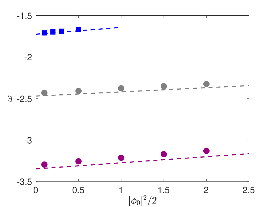
In figure 13, the modified eigenfrequency that takes the wave-feedback into account, i.e. $\omega=\omega_{0}+\tilde{\omega}$ , is compared against the frequency of slow modulations in Boussinesq simulations. Three sets of simulations are considered where all the parameters are fixed within each set while the initial wave energy ${\left|\phi_{0}\right|^{2}}/2$ is varied. These results show good agreement between the nonlinear coupled model of Xie and Vanneste 2015 and the Boussinesq simulations and confirm the validity of (36). There is a small offset between the predicted and simulation frequencies of some sets, which is due to the issues (i)-(iii) discussed in the previous section. For ‘L8c-R04’ (the blue markers) in figure 13 the analysis is limited to $E_{0}<0.5$ : as discussed in the conclusion, for higher amplitude waves the vortex strongly interacts with the near inertial wave.

5 Conclusion and discussion

The linearized YBJ model of section 2 focusses attention on the back-rotated velocity – rather than the radial velocity – as the simplest variable characterizing the trapped eigenmodes of an anticyclonic vortex. This is in immediate agreement with solutions of the Boussinesq equations: the top row of figure 1 shows that the trapped disturbance does not have a conspicuous radial velocity component. Instead, the back-rotated velocity is approximately independent of azimuth. Thus the advective term, $J(\psi,\phi)$ in (5), vanishes identically so that near-inertial trapping results only from the $\mathrm{i}\zeta\phi/2$ frequency shift. In section 2 2.4 we show that as a consequence the lowest possible frequency of the vortex eigenmode – the “bottom of the discrete spectrum” – is $f+\zeta_{\mathrm{min}}/2$ .

Exquisite excitation of a single pure eigenmode produces a steady (time-independent) axisymmetric pattern of wave kinetic energy density. But generic forcing or initial conditions excites all of the available discrete modes of the vortex, and also a continuum of untrapped disturbances. Thus in the top row of figure 2 we see that the initial condition in (3) – chosen to represent excitation by an atmospheric storm of scale much larger than the vortex scale – results in a low-frequency pulsation of the kinetic energy density, corresponding to the oscillations in the wave kinetic energy time series of figure 3. This pulsation is not a single pure eigenmode. In section 3 we extracted the frequency of the sub-inertial oscillation from figure 3 and showed that this modal period is in good agreement with the predictions of the YBJ equation.

In section 4 we go beyond the linear approximation and test the predictions of the phase-averaged model of Xie and Vanneste 2015, Wagner and Young 2016 and Rocha et al. 2018. This model couples quasigeostrophic and YBJ models and accounts for the mean-flow change induced by wave feedback (Kafiabad et al. 2020, see also) through a wave contributions to PV. We show that the wave feedback leads to frequency shift of the vortex eigenmode that is linearly proportional to the kinetic energy of the eigenmode. We find this frequency shift is in good quantitative agreement with Boussinesq results. This confirms the ability of the phase-averaged coupled model to represent NIW–mean flow interactions.

All results in this work are in the regime of weak nonlinearity. But what happens if one hits the vortex with a very large initial disturbance? Figures 14 and 15 show the result of strongly perturbing a Gaussian vortex by increasing the amplitude of the initial condition $\phi_{0}$ in (3). The initial development of this large disturbance, up to about 55 inertial periods, is similar to that of the weakly nonlinear problem shown in the top row of figure 2: the wave kinetic energy concentrates in the vortex core and the barotropic vorticity remains smooth. But after about 60 inertial periods the core concentration of wave kinetic energy triggers an instability – see figure 15. The high-frequency bursts in figure 15 are accompanied by the formation of small spatial scales in the vorticity field: in figure 14 (j), (k) and (l), the main anticyclone curdles and small vortex dipoles circulate around its crumbled remains. It is impressive that a prominent sub-inertial cycle persists and that there are episodes of “relaminarization” coincident with the wave-energy minima in figure 15. This low-frequency modulation of the instability is a persistent signature of the vortex eigenmode that survives for over 300 inertial periods. There are open questions about the nature of the instability observed in figure 14 which we leave for future work.

Data availability statement.

Acknowledgements.

HAK and JV are supported by the UK Natural Environment Research Council grant NE/R006652/1. WRY is supported by the National Science Foundation Award OCE-1657041. This work used the ARCHER UK National Supercomputing Service. [A] \appendixtitleThe weak-trapping limit We solve the eigenvalue problem (14) in the weak-trapping regime

\sigma\ll 1

using matched asymptotics. In the outer region,

\eta\gg 1

, the Gaussian vorticity is exponentially small and can be neglected. This leads to the outer approximation

A(\eta)=qK_{0}\left(\sqrt{\sigma}\,\eta\right)\,,

(38)

where $K_{0}$ is the modified Bessel function and $q$ is undetermined constant. In an intermediate region where $\sqrt{\sigma}\,\eta\ll 1$ and $\eta\gg 1$ , the Bessel function $K_{0}$ is approximated as

A(\eta)=-q\ln\eta-\tfrac{1}{2}q\ln\sigma+q\big(\ln 2-\gamma_{\mathrm{E}}\big)+\cdots,

(39)

where $\gamma_{\mathrm{E}}$ is Euler’s constant and we have used the small-argument asymptotics of $K_{0}$ .

In the inner region where $\eta=O(1)$ , we use $\sigma\ll 1$ to reduce (14) to

\frac{\mathrm{d}^{2}A}{\mathrm{d}\eta^{2}}+\frac{1}{\eta}\frac{\mathrm{d}A}{\mathrm{d}\eta}+\lambda\mathrm{e}^{-\eta^{2}}A=0\,.

(40)

We select the bounded solution as $\eta\to 0$ by imposing

A(0)=1\quad\textrm{and}\quad A^{\prime}(0)=0\,.

(41)

Equations (40) and (41) define an initial-value problem which – except of the zeroth mode in (46) below – must be solved numerically. For $\eta\gg 1$ , the solution has the asymptotics

A(\eta)\sim\alpha(\lambda)\ln\eta+\beta(\lambda)+o(1),

(42)

with $\alpha(\lambda)$ and $\beta(\lambda)$ determined from the numerical solution. Matching (42) with (39) results in

\frac{\beta(\lambda)}{\alpha(\lambda)}=\tfrac{1}{2}\ln\sigma+\gamma_{\mathrm{E}}-\ln 2\,.

(43)

This is an equation for $\sigma$ that is valid only for $\beta/\alpha<0$ and $|\beta/\alpha|\gg 1$ so that $\sigma\ll 1$ as assumed. Equation (43) identifies the zeros $\lambda_{n},\ n=0,\,1,\cdots$ of the function $\alpha(\lambda)$ as the values of $\lambda$ at which new branches of the dispersion relation appear. Note that $\lambda_{0}=0$ corresponds to the zeroth mode; this eigensolution exists even for very weak vortices.

We have computed $\alpha$ and $\beta$ numerically for $0<\lambda\leq 40$ and show the results in figure 5. The first bifurcation values of $\lambda$ are found to be $\lambda_{0}=0$ , $\lambda_{1}\approx 11.1$ and $\lambda_{1}\approx 35.1$ . In view of the sign of $\beta(\lambda_{n})$ , new branches appear for $\lambda>\lambda_{n}$ . Approximating the left-hand side of (43) near $\lambda_{n}$ and solving for $\sigma$ leads to the dispersion relations

\sigma\sim e^{2(\ln 2-\gamma_{\mathrm{E}})-c_{n}/(\lambda-\lambda_{n})}\quad\textrm{as}\ \ \lambda\to\lambda_{n}^{+},

(44)

with $c_{n}=-2\beta(\lambda_{n})/\alpha^{\prime}(\lambda_{n})>0$ .

We can obtain a fully analytic form for the $n=0$ branch (the zeroth mode), with $\lambda\approx\lambda_{0}=0$ by solving (40) asymptotically for $\lambda\ll 1$ . A straightforward expansion in powers of $\lambda$ gives

	$\displaystyle A(\eta)$	$\displaystyle=1-\frac{\lambda}{4}\int_{0}^{\eta^{2}}\frac{e^{-x}-1}{x}\,\mathrm{d}x+O(\lambda^{2})\,,$		(45)
		$\displaystyle=1-\tfrac{1}{4}\lambda\left(E_{1}(\eta^{2})+2\ln\eta\right)+O(\lambda^{2})\,,$		(46)

where $E_{1}$ is the exponential integral. Noting that $E_{1}(\eta)\to 0$ as $\eta\to\infty$ , we find from (42) that as $\lambda\to 0$ , $\alpha(\lambda)\sim-\lambda/2$ and $\beta(\lambda)\sim 1$ ; this results in $c_{0}=4$ and the zeroth-mode dispersion relation in (17). For the $n=1$ branch, we find numerically $\alpha^{\prime}(\lambda_{1})\approx 0.18$ and $\beta(\lambda_{1})\approx-0.62$ ; hence $c_{1}\approx 6.8$ .

[B] \appendixtitleFrequency shift due to wave feedback

Substituting (34) into (33), and keeping the terms at order $\varepsilon^{0}$ , leads to

-\omega_{0}A_{0}+\frac{1}{2}\triangle\psi_{0}A_{0}-\frac{1}{2}\hbar\triangle A_{0}=0,

(47)

which is the dimensional form of (14) for $A_{0}$ and $\omega_{0}$ . Based on this equation, we introduce the self-adjoint operator $\mathcal{L}$

\mathcal{L}=-\omega_{0}+\frac{1}{2}\triangle\psi_{0}-\frac{1}{2}\hbar\triangle.

(48)

The terms at the next order form the following equation

-\tilde{\omega}A_{0}+\frac{\mathcal{L}\tilde{\phi}}{\alpha_{0}\phi_{0}}-\frac{\alpha_{0}^{2}{\left|\phi_{0}\right|^{2}}}{8f}\triangle A_{0}^{2}\ A_{0}=0,

(49)

which can be multiplied by $A_{0}$ and then integrated to obtain

\displaystyle-\tilde{\omega}\int A_{0}^{2}\,r\mathrm{d}r+\int(\mathcal{L}\tilde{A})A_{0}\,r\mathrm{d}r-\frac{1}{8f}\int A_{0}^{2}\ \triangle A_{0}^{2}\,r\,\mathrm{d}r=0

(50)

(All integral run from $r=0$ to $\infty$ ). Because of the self-adjoint property of $\mathcal{L}$ and (47),

\int(\mathcal{L}\tilde{\phi})A_{0}r\,\mathrm{d}r=\int\tilde{\phi}(\mathcal{L}A_{0})r\,\mathrm{d}r=0.

(51)

The last integral in (50) can also be simplified after integration by parts

	$\displaystyle\int A_{0}^{2}\triangle A_{0}^{2}\ r\,\mathrm{d}r$	$\displaystyle=\int A_{0}^{2}\frac{\mathrm{d}}{\mathrm{d}r}\left(r\frac{\mathrm{d}}{\mathrm{d}r}A_{0}^{2}\right)\,\mathrm{d}r$
		$\displaystyle=-\int\left(\frac{\mathrm{d}}{\mathrm{d}r}A_{0}^{2}\right)^{2}\ r\,\mathrm{d}r$		(52)

Using (51) and (5), (50) reduces to the following expression after rewriting the integrals in terms of the dimensionless coordinate $\eta=r/a$

\tilde{\omega}=\frac{{\left|\phi_{0}\right|^{2}}}{8fa^{2}}\cfrac{\left(\mathop{{\int}}A_{0}\eta\mathrm{d}\eta\right)^{2}\mathop{{\int}}\left(\cfrac{\mathrm{d}}{\mathrm{d}\eta}A_{0}^{2}\right)^{2}\eta\mathrm{d}\eta}{\left(\mathop{{\int}}A_{0}^{2}\eta\mathrm{d}\eta\right)^{3}},

(53)

where we used (27) to substitute for $\alpha_{0}$ .

References

Asselin and Young (2020) Asselin, O., and W. R. Young, 2020: Penetration of wind-generated near-inertial waves into a turbulent ocean. Journal of Physical Oceanography.
Chavanne et al. (2012) Chavanne, C. P., E. Firing, and F. Ascani, 2012: Inertial oscillations in geostrophic flow: Is the inertial frequency shifted by $\zeta$ /2 or by $\zeta$ ? Journal of Physical Oceanography, 42, 884–888.
Danioux et al. (2015) Danioux, E., J. Vanneste, and O. Bühler, 2015: On the concentration of near-inertial waves in anticyclones. Journal of Fluid Mechanics, 773.
Elipot et al. (2010) Elipot, S., R. Lumpkin, and G. Prieto, 2010: Modification of inertial oscillations by the mesoscale eddy field. Journal of Geophysical Research: Oceans, 115 (C9).
Joyce et al. (2013) Joyce, T. M., J. M. Toole, P. Klein, and L. N. Thomas, 2013: A near-inertial mode observed within a gulf stream warm-core ring. Journal of Geophysical Research: Oceans, 118 (4), 1797–1806.
Kafiabad et al. (2020) Kafiabad, H. A., J. Vanneste, and W. R. Young, 2020: Wave-averaged balance: a simple example. arXiv preprint arXiv:2003.03389.
Kunze (1985) Kunze, E., 1985: Near-inertial wave propagation in geostrophic shear. Journal of Physical Oceanography, 15 (5), 544–565.
Kunze and Boss (1998) Kunze, E., and E. Boss, 1998: A model for vortex-trapped internal waves. Journal of Physical Oceanography, 28 (10), 2104–2115.
Kunze et al. (1995) Kunze, E., R. W. Schmitt, and J. M. Toole, 1995: The energy balance in a warm-core ring’s near-inertial critical layer. Journal of Physical Oceanography, 25 (5), 942–957.
Lee and Niiler (1998) Lee, D.-K., and P. P. Niiler, 1998: The inertial chimney: The near-inertial energy drainage from the ocean surface to the deep layer. Journal of Geophysical Research: Oceans, 103 (C4), 7579–7591.
Llewellyn Smith (1999) Llewellyn Smith, S. G., 1999: Near-inertial oscillations of a barotropic vortex: trapped modes and time evolution. Journal of Physical Oceanography, 29 (4), 747–761.
Rocha et al. (2018) Rocha, C. B., G. L. Wagner, and W. R. Young, 2018: Stimulated generation: extraction of energy from balanced flow by near-inertial waves. Journal of Fluid Mechanics, 847, 417–451.
Wagner and Young (2015) Wagner, G., and W. R. Young, 2015: Available potential vorticity and wave-averaged quasi-geostrophic flow. Journal of Fluid Mechanics, 785, 401–424.
Wagner and Young (2016) Wagner, G. L., and W. R. Young, 2016: A three-component model for the coupled evolution of near-inertial waves, quasi-geostrophic flow and the near-inertial second harmonic. Journal of Fluid Mechanics, 802, 806–837.
Xie and Vanneste (2015) Xie, J.-H., and J. Vanneste, 2015: A generalised-Lagrangian-mean model of the interactions between near-inertial waves and mean flow. Journal of Fluid Mechanics, 774, 143–169.
Young and Ben Jelloul (1997) Young, W. R., and M. Ben Jelloul, 1997: Propagation of near-inertial oscillations through a geostrophic flow. Journal of Marine Research, 55 (4), 735–766.
Zhai et al. (2005) Zhai, X., R. J. Greatbatch, and J. Zhao, 2005: Enhanced vertical propagation of storm-induced near-inertial energy in an eddying ocean channel model. Geophysical Research Letters, 32 (18).